Efficient sequential sampling for global optimization in static and dynamic environments

(1)

University of Warwick institutional repository: http://go.warwick.ac.uk/wrap

A Thesis Submitted for the Degree of PhD at the University of Warwick

http://go.warwick.ac.uk/wrap/62123

This thesis is made available online and is protected by original copyright.

Please scroll down to view the document itself.

(2)

Efficient sequential sampling for global optimization

in static and dynamic environments

by

Sergio Morales Enciso

Thesis

Submitted to the University of Warwick

for the degree of

Doctor of Philosophy

Complexity Sciences and Operational Research

(3)

List of Tables

3.1 SPEGO - Initial DoE . . . 54

3.2 SPEGO - Partitioning dimension selection criteria . . . 56

3.3 SPEGO - Partitioning threshold as a function of problem dimension 58 3.4 SPEGO - Effect of partitioning threshold size . . . 58

3.5 SPEGO vs. NSPEGO . . . 64

3.6 SPEGO vs. EGO . . . 65

3.7 SPEGO vs. CMA-ES vs. SMAC . . . 71

4.1 Parameters for the moving peaks benchmark . . . 88

(7)

List of Figures

2.1 Expected improvement illustration . . . 17

2.2 Comparison of EGO with different fixed solution qualities for the expected improvement . . . 20

2.3 Comparison of EGO with random solution qualities for the expected improvement . . . 21

2.4 Number of local maxima in EI as a function of sample size . . . 23

2.5 Fixed target vs. fixed cost paradigms . . . 26

2.6 Illustration of the random multi-start and hyper-box methods . . . . 27

2.7 Comparison of the random multi-start, hyper-box, and genetic algo-rithm optimization methods to optimize the expected improvement . 32 2.8 Comparison for restricted EI function evaluations budget of the three proposed EI maximization techniques . . . 34

3.1 Space partitioning illustration . . . 48

3.2 SPEGO - Initial DoE . . . 55

3.3 SPEGO - Dimension selection criteria . . . 57

3.4 SPEGO - Threshold partitioning size - Performance . . . 60

3.5 SPEGO - Threshold partitioning size - Running time . . . 61

3.6 SPEGO vs. NSPEGO - Performance . . . 62

3.7 SPEGO vs. NSPEGO - Running time . . . 63

3.8 SPEGO vs. EGO - Fixed time comparison . . . 66

3.9 SPEGO vs. EGO - Fixed budget comparison . . . 68

3.10 SPEGO vs. EGO - Running time . . . 69

(8)

4.1 Sequential sampling using DIN strategy illustration (low noise) . . . 82

4.2 Sequential sampling using DIN strategy illustration (high noise) . . . 83

4.3 Noise level optimization for DIN sampling strategy . . . 90

4.4 Offline and average errors for all strategies - 1D . . . 91

4.5 Offline error convergence curves . . . 93

4.6 Current error for each compared strategy - Individual plots . . . 94

4.7 Offline error for the parameter analysis - 1D . . . 96

4.8 Offline error for the parameter analysis - 2D . . . 97

A.1 SPEGO vs. CMA-ES vs. SMAC - Separable functions . . . 108

A.2 SPEGO vs. CMA-ES vs. SMAC - functions with low or moderate conditioning . . . 109

A.3 SPEGO vs. CMA-ES vs. SMAC - functions with high conditioning and unimodal . . . 110

A.4 SPEGO vs. CMA-ES vs. SMAC - multi-modal functions with ade-quate global structure . . . 111

(9)

Acknowledgments

I would like to express my deepest appreciation to Professor Juergen Branke, my

main supervisor, for his wise advice, bright ideas, continuous encouragement, and

unrestricted availability, all of which made this accomplishment possible.

I am also extremely grateful to Professor Robin C. Ball, my co-supervisor,

for his invaluable insights, and all the help and support provided throughout my

years at the Centre for Complexity Science.

For encouraging me to consider the path of research, I would like to thank

Dr. Enrique Garza Escalante.

For their unconditional support, I am ever grateful to my family. In

par-ticular, to my mother for instilling into me the passion for creativity, and showing

me that imagination is more powerful than knowledge. And to my father, who

through his example, taught me the value of rightness, hard work, and importance

(10)

Declarations

This thesis is submitted to the University of Warwick in support of my application

for the degree of Doctor of Philosophy. It has been composed by myself and has not

been submitted in any previous application for any degree. Every effort has been

made to credit the authors of the published work which provides the foundations

upon which this research is built.

The work presented (including data generated and data analysis) was carried out

by the author.

Parts of this thesis have previously been published, or have been submitted for

publication, by the author:

• Morales-Enciso, S. and Branke, J. Response Surfaces with Discounted

Infor-mation for Global Optima Tracking in Dynamic Environments. In Nature

Inspired Cooperative Strategies for Optimization (NICSO 2013), vol. 512 of

Studies in Computational Intelligence, pp. 57–69. Springer International

Pub-lishing, 2014. doi: 10.1007/978-3-319-01692-4

• Morales-Enciso, S. and Branke, J. Tracking global optima in dynamic

environ-ments with efficient global optimization. Submitted to theEuropean Journal

of Operational Research, November 2013.

(11)

Abstract

Many optimization problems involve acquiring information about the under-lying process to be optimized in order to identify promising solutions. Moreover, in some cases obtaining this information can be expensive, which calls for a method capable of predicting promising solutions so that the global optimum can be found with as few function evaluations as possible. Another kind of optimization problem arises when dealing with objective functions that change over time, which requires tracking of the global optima over time. However, tracking usually has to be quick, which excludes re-optimization from scratch every time the problem changes. In-stead, it is important to make good use of the history of the search even after the environment has changed.

(12)

List of Abbreviations

ANN Artificial Neural Networks

APRS Adaptive partitioning random search

BBOB Black-box optimization benchmark

CMA-ES Covariance matrix adaptation for evolution strategies

DoE Design of experiments

EA Evolutionary algorithm(s)

ECDF Empirical cumulative density function

EGO Efficient Global Optimization

EI Expected improvement

GA Genetic algorithm

GP Gaussian process(es)

HB Hyper-box multi-start with local hill climbers

IAGO Informational approach to global optimization

KGCB Knowledge gradient-policy for correlated beliefs

KGCP Knowledge gradient for continuous parameters policy

LHS Latin hypercube sampling

(13)

MARS Multivariate adaptive regression splines

NP Nested partitioning

NSPEGO Non-disjoint space partitioning efficient global optimization

PR Polynomial regression

PRS Pure random sampling

RBF Radial Basis Functions

RMS Random multi-start (with local hill climbers)

RS Random sampling

SA Simulated annealing

SMAC Sequential model-based algorithm configuration procedure

SPEGO Space partitioning efficient global optimization

SS Stratified sampling

(14)

Chapter 1

Introduction

Optimization is the process of finding the best alternative, out of all feasible

al-ternatives, with respect to previously defined criteria. However, finding the best

alternative (here called solution) is rarely trivial. Optimization is ubiquitous, but

its presence is often overlooked. For instance, parcel delivery, air traffic control

sys-tems, search engines, timetable assignments, and unmanned aerial vehicles, all have

in common that they rely on solving optimization problems.

In order to tackle optimization problems algorithmically, it is convenient to

state them in a mathematical way, where the decisions to be made are modeled as

independent variables or parameters. When evaluating the problem at a given set

of parameters, the observed outcome represents a dependent variable, or response

value. The pair formed by this outcome, together with the parameter setting used to

obtain it, is referred to as a sample or an observation, and the function mapping the

space of all parameters to their corresponding response value, as objective function.

When the objective function is a simulation model, or represents an unknown

natural process, an analytic representation is usually not available. Such

optimiza-tion problems are often referred to as black-box optimizaoptimiza-tion problems. The lack

of analytic representation restricts the use of gradient based optimization methods.

Instead, during optimization, it is necessary to learn about the characteristics of

the objective function via sampling. The learning process can be implemented in

different ways, one of which is to use statistical techniques capable of inferring and

(15)

an approximation of the value of a function at a given location.

In some cases, obtaining information about the system is costly. We

re-fer to these cases as expensive-to-evaluate due to the amount or type of resources

needed to acquire new information, which most often involves large investments,

long waiting times, human resources, or disruptions to a system.

Expensive-to-evaluate optimization problems are likely to arise, for example, when dealing with

complex simulations or in engineering design [Burl and Wang, 2009]. For instance,

improving the design of a wing, a nano-pipe, or a car frame, which is controlled by a

set of parameters that are to be optimized, usually involves running computational

fluid dynamics simulations that may take hours to run. In this example, the cost is

measured in time. Another common scenario is the identification of promising

re-gions for mining, where data collection involves sending out workers for excavations,

chemical analyses or data processing. Not only is this time consuming but it also is

expensive in monetary terms.

Shan and Wang [2009] conclude that current research does not focus on

try-ing to directly model and understand black-box functions, but rather focuses on

improving sampling strategies and finding clever uses of the scarce observed data in

order to determine promising areas to explore. This coincides with the main topic

of the current thesis which is to determine efficient sequential sampling policies and

to study their practical implementation under different situations. The sampling

strategies presented throughout this thesis are based on the well-studied field of

sequential Bayesian optimization, which is a general probabilistic approach for

es-timating unknown probability density functions in a recursive manner over time,

using data to update the estimated model progressively, as it becomes available.

The main contributions of this thesis are, first, a quantitative study showing

the benefits of finding the global maximum of the expected improvement, an

aux-iliary function that arises as part of the selected response-surface-aided sequential

optimizer. Second, the conception, design, analysis, and benchmark of SPEGO,

a response-surface-aided sequential sampling optimization algorithm that extends

the well established Efficient Global Optimization (EGO) algorithm. The proposed

(16)

compu-tational complexity as a function of the number of samples, to linear, with only a

minor impact on the quality of the solutions it finds. And third, we propose the first

approach to track the global optima of dynamically changing optimization problems

by means of a surrogate-based global search algorithm.

This thesis is structured as follows. Chapter 2 starts by presenting a

liter-ature survey on response surface modeling, which reveals that the static version of

the black-box optimization problem has been extensively studied. Then, the

nec-essary terminology and notation to approach this problem is introduced, providing

the theoretical background and fundamental building blocks required to treat more

sophisticated versions of the problem in later chapters. Besides, the methodology

selected to benchmark the algorithms thoroughout the rest of the thesis is explained,

demonstrating its use by exploring the impact of an important parameter governing

the chosen sequential optimization algorithm.

In Chapter 3 we propose a new algorithm, based on space partitioning, so

as to accelerate the response surface aided sequential optimization process. After

introducing the main concepts for partitioning the space, different enhancements and

implementation decisions are tested through numerical experimentation. Then, the

proposed algorithm is benchmarked against both the original algorithm it extends,

and state of the art algorithms encountered in the literature.

Chapter 4 is devoted to the study of dynamic environments where, rather

than finding the global optimum, the goal is to track the changing optimum over

time. This chapter starts by presenting a literature review on dynamic optimization

of black-box functions, followed by the detailed presentation of several methods to

adapt the response surface based optimization techniques introduced in previous

chapters. Then, the performance of these methods is evaluated using a benchmark

specifically designed for dynamic environments, and a statistical study of the results

obtained through numeric experimentation is presented.

Finally, Chapter 5 provides some concluding notes and proposes future

(17)

Chapter 2

Global optimization of

expensive-to-evaluate black-box

functions

As outlined in the introductory chapter, global optimization is a very broad term

which tackles the problem of finding the best solution, in the solution set, of an

objective function. Best, in this context and without loss of generality, refers to

either the minimum or the maximum of such an objective function, depending on

the nature of the problem at hand.

The field of global optimization is vast, and the problems it addresses vary

so much that many sub-fields have emerged. A good survey on recent advances in

some sub-fields of global optimization can be found in Floudas and Gounaris [2008].

Since the main focus of the current thesis is to study efficient strategies

for finding the global optima of deterministic functions of which the structure is

not known, and which are expensive to evaluate, we devote this first chapter to

introduce the basic concepts that arise in the context of this specific sub-field of

optimization. More specifically, we present a review of the state of the art of the

existing methodologies, we establish the terminology that will be used throughout

the remainder of the thesis, and we justify the selection of a good response surface

methodology coupled with a sequential algorithm to be used as a base to develop new

(18)

context of the current research with respect to the whole field of global optimization,

and points to related techniques that have been applied to solve similar problems.

In Section 2.2, the concept of design of experiments is outlined, which, together with

the response surface methodologies introduced and studied in Section 2.3, serve as a

starting point to understand the idea behind sequential sampling for optimization.

Since sequential sampling for optimization is at the core of the ideas discussed

all throughout this thesis, it is explained in detail in Section 2.4, where different

approaches are compared, and justifications for the selected method are provided.

Then, the subproblem arising when choosing new locations to sample is thoroughly

addressed in Sections 2.5 and 2.6, the latter serving as well to introduce a widely

accepted benchmark and useful performance measures. Finally, some concluding

notes and remarks are given in Section 2.7.

2.1 Global optimization of expensive-to-evaluate

black-box functions

In a recent article, S¨orensen [2013] proposed that algorithms for global optimization

can be classified into three categories (exact algorithms, heuristic algorithms, and

approximation algorithms), explaining that exact algorithms guarantee to find an

optimal solution in a finite amount of time, whereas heuristics do not provide this

guarantee at all, and approximation methods can only guarantee to find a solution

within some arbitrary precision of the real optimum. While this classification is

accurate, it fails to consider algorithms that guarantee finding optimal solutions in

infinite time, which are usually stochastic methods (e.g. simulated annealing

[Kirk-patrick, Gelatt, and Vecchi, 1983]), or space filling iterative methods such as the one

that is the subject of study in this thesis and for which Locatelli [1997] presented a

proof of convergence in infinite time. However, care must be taken when considering

infinite time horizons, and for practical purposes, algorithms falling in this category

shall be considered heuristics.

The term black-box describes a system of which the internal functioning and

(19)

responses obtained for the provided inputs. Due to the lack of an analytic expression

for black-box objective functions, methods requiring an analytic expression of the

objective function or of its gradient can not be applied. This leaves heuristics and

approximation methods as the only approaches for optimizing black boxes. There is

a plethora of heuristics and approximation methods that have been proposed. Below

only some of the most widespread and commonly found in literature are briefly

explained, and a deeper review on approximation methods is left for Section 2.3.

• Pure random sampling (PRS): Points within the feasible space are sampled

uniformly at random. This is applicable to most problems since no

assump-tions need to be made about the search space. Nevertheless, this approach

tends to be very slow since no adaptation nor learning about the structure

of the problem at hand is done. For a review on these methods and proof of

convergence, see Solis and Wets [1981].

• Simulated annealing (SA): First proposed by Kirkpatrick, Gelatt, and Vecchi

[1983], this algorithm, which mimics the annealing process of solids, explores

the search space by always accepting local movements towards states with

better solutions and accepting local movements towards states with worse

so-lutions with a positive probability that decreases according to a predefined

schedule. Being able to accept movements with worse solutions is what

pre-vents the algorithm from getting trapped in local optima, and allows a more

extensive search of the optimal solution. As in PRS, no explicit adaptation nor

learning is done during the search process, although local structure is exploited

through local movements towards better states.

• Evolutionary algorithms (EA): As explained by Spears, de Jong, and B¨ack

[1993], the term EA is a term used to refer to a variety of heuristic algorithms

inspired by the processes of natural evolution, and amongst others, includes

genetic algorithms, evolutionary programming, and genetic programming.

Al-though they differ in the details and in many aspects, all these algorithms share

the basic idea of keeping a population of individuals which evolves according

to some rules of selection such as mutations and crossovers. With the aim of

(20)

according to a fitness function so that the fittest individuals under such a

mea-sure are somehow given preference to survive and/or reproduce. Mutations

and crossover, being random, help avoiding premature local convergence.

• Response surface modeling: Unlike all the previous outlined methods which at

best use some sort of memory to keep track of good regions within the feasible

space, creating a response surface using the available data allows learning of

the structure of the landscape by studying the existing correlations amongst

observations. Different techniques for doing so exist, and in general they

in-volve some type of regression which is used for the inference part (fitting a

response surface to the data), and a criterion to select where the new

obser-vations shall be made based on the inferred surface. Exploiting the structure

of the landscape provides an advantage to this technique when compared to

the previously mentioned optimization techniques, which is a great advantage

when dealing with a limited number of samples. However, this advantage

comes at the cost of having to spend more time and computational effort in

both building the response surface, and selecting the locations for the next

observations. Since response surface based optimization is a central topic of

this thesis, a more thorough discussion can be found in Section 2.3.

2.2 Initial design of experiments for sequential

sam-pling optimization

In a broad sense, design of experiments (DoE) is a systematic method for selecting

which data should be collected and how it should be collected during an experiment,

usually with the goal of inferring as much information as possible from the responses

obtained subject to a fixed budget in terms of number of samples. More traditional

DoE focuses on selecting the data collection points before the experiment starts

(off-line) while sequential sampling dynamically selects the location of the next sample

each time new data is available (on-line). However, even the latter requires a few

samples before it can actually build a useful model to start the on-line process for

(21)

Methods for selecting this initial set of samples have been widely studied

under the umbrella of DoE. These methods assume a budget, measured for instance

in number of samples to be taken, that we shall call λ, and aim to distribute them

throughout the feasible space so as to obtain as much information as possible.

De-pending on how information is characterized, this leads to different criteria to be

optimized. However, since most of the response surface enhanced optimization

mod-els require only a reduced number of initial samples to start the infill process1, these

methods do not have much influence on the final result. So we describe only three

settings popular in both the DoE and the sequential optimization communities, but

point the interested reader to Pukelsheim [2006] for a thorough enumeration of DoE

criteria with detailed definitions.

• Random sampling (RS): Points are drawn uniformly at random from the

fea-sible space, without any restriction. This might lead to some samples being

close to each other and to leave some regions unexplored. No partitioning of

the space is required, and it is straightforward to implement.

• Stratification, or stratified sampling (SS): The feasible space is first partitioned into disjoint strata (or regions), and then random sampling is applied in each

stratum with a local sampling budget proportional to the size of the region.

Using this technique, all regions of the feasible space will be represented. In

some cases, the partitions might be meaningful and arise naturally from the

problem at hand, however, when dealing with generic black-box functions the

partitions might seem arbitrary. Raj [1968] offers a deeper explanation on

this technique. SS designs can require a very large number of samples when

dealing with a large number of dimensions.

• Latin hypercube sampling (LHS): Introduced by McKay, Beckman, and Conover

[1979], the idea is to divide each input variable (or dimension) into ranges so

as to create partitions of the feasible space, and then choose in which regions

to get the samples. The selection of the regions to be sampled must satisfy the

1

(22)

Latin hypercube property, which means that exactly one sample of each range

will be randomly taken. This is the generalization to many dimensions of the

Latin square sampling method [Raj, 1968]. In doing so, LHS ensures not only

that —when considering a given single dimension— all portions of the feasible

space are sampled, but also that each of the ranges from all the input variables

are represented. Since LHS does not aim to sample all the regions created by

the intersection of the chosen ranges in all dimensions simultaneously —unlike

SS—, the number of samples required to create a sampling design remains

relatively low even for a large number of dimensions.

In general, DoE techniques aim to distribute the samples in order to get

the best approximation of the whole space, but this does not necessarily help when

seeking to optimize an expensive-to-evaluate black-box function since the interest is

rather in obtaining good approximations only around the good regions, and ideally,

samples should not be wasted in accurately modeling bad regions. This is why

we focus on sequential sampling strategies which, given an initial design, provide a

location for the next most promising sample. So, in the remainder of this chapter,

the initial design is obtained using random sampling, with a budget for this initial

stage large enough only to allow for fitting a response surface model, and the use of

LHS as an initial DoE is delayed to Chapter 3.

2.3 Gaussian processes as response surfaces

for optimization

Response surfaces (or surrogate models) are approximations of an objective function

created using available data, and are the output of some sort of regression. These

models are used when a direct measurement of the function is not practical, for

instance, if each measurement is expensive to obtain in time, money, or any other

cost unit.

Many different techniques to build response surfaces have emerged in the

recent years, so in this section we first review some of the most widely used response

surface techniques, and then present the one of our choice, Gaussian processes (GP),

(23)

2.3.1 Response surface methodologies

Response surface optimization has now been studied for a long time, and many

techniques have been proposed, some of which have been enhanced, refined, and

tailored for specific problems throughout the years. However, the basic techniques

for fitting response surfaces remains the same and in most of the cases falls within

one of the following classes.

Polynomial regression (PR) is perhaps the oldest response surface method,

dating back to 1805 and 1809 when Legendre and Gauss independently proposed

it, but it was not until the 20th century that it was popularized as a DoE method

[Smith, 1918]. Other techniques include, but are not limited to, least interpolating

polynomials (LIP) [Boor and Ron, 1990], multivariate adaptive regression splines

(MARS) [Friedman, 1991], artificial neural networks (ANN) [Papadrakakis, Lagaros,

and Tsompanakis, 1998], support vector machines (SVM) [Drucker, Burges,

Kauf-manet al., 1997; Cristianini and Shawe-Taylor, 2000], radial basis functions (RBF)

[Dyn, Levin, and Rippa, 1986; Fang and Horstemeyer, 2006], and GP (also known

as kriging) [Jones, Schonlau, and Welch, 1998].

Comprehensive and detailed surveys on response surface modelling for global

optimization are provided by Jones [2001],Wang and Shan [2007], Shan and Wang

[2009], and Lim, Jin, Memberet al. [2010].

2.3.2 Gaussian processes

One reason to choose GP as a method to build response surfaces is that it is a

non-parametric regression technique, which is an advantage over methods like PR,

LIP, and MARS when dealing with black-box functions. Furthermore, GP provide

analytical tractability not only for the predictions but also for the confidence on its

predictions, an essential requirement for the Efficient Global Optimization algorithm

to work (to be introduced in Section 2.4.2), which SVM and ANN can not provide.

Finally, GP set a natural framework to incorporate old information for the dynamic

case as is proposed in Section 4.2.

GP, just like all the other techniques, take as an input a set of observations

(the dataset) that we shall denote as D, which is composed by N ∈ _N pairs of

(24)

corresponding observed response, or dependent variable, yn ∈ R. The available

observations inD, which is defined as

D={(xn, yn)nN=1}={X,Y}, (2.1)

are considered a training set, from which the model learns. As an output,

the model aims to provide a prediction or estimate of the dependent variable ˆyp∈R

at any other test pointxp ∈RD.

Formally, a GP is fully defined by a mean function which allows introduction

of any prior information available into the model, and a covariance function (or

kernel) which expresses the scaled correlation between the data points [Rasmussen

and Williams, 2006]. As a result of applying GP for regression to a dataset, we

obtain a random functionf` distributed as a Gaussian process with mean function

m(x), and covariance function k(x,x0), which is denoted as

f`∼ GP(m(x), k(x,x)). (2.2)

Unless otherwise stated, throughout this thesis, a zero mean prior function

m(x) = 0 (2.3)

and the squared exponential covariance function

k(x,x0) =σ_f2exp

− D

X

d=1

(xd−x0d)2

2`2

d

+σ_n2δ(x,x0) (2.4)

are used, whereδ(x,x0) is the Kronecker delta function, and is defined as

δ(x,x0) =

 



0 if x6=x0

1 if x=x0. (2.5)

The zero mean prior function is chosen —without loss of generality— to

simplify the equations, however this is not a requirement, and arbitrary mean prior

functions can be used, as it is done in Section 4.2.7. The kernel function can be

(25)

calculated for every possible pair of samples and gives rise to the covariance matrix

K. However, the covariance matrix will typically have some free parameters that,

lacking any prior knowledge, can only be estimated from the data. Considering

Equation (2.4), there areD+ 2 parameters to be learnt. These parameters include

the signal varianceσ_f2 ∈_Rwhich determines the maximum covariance of the process,

the measurement noise variance σ2_n ∈ _R which quantifies how noisy the process

generating the samples is and can be set to zero for the deterministic case, and a

characteristic length-scale for each dimension```= [`1, ..., `D]∈RD which dictates in what measure two data samples correlate to each other as a function of the distance

separating them. For convenience, we aggregate all the parameters in the vector

θ

θθ= [σ2_f, σ_n2, ```]∈_RD+2. (2.6)

A common way for estimating θθθ is to choose the set of parametersθθθ∗ that

maximize the probability of the data being generated by a GP given such a set of

parameters. This can be done by maximizing the marginal likelihood, or

equiva-lently, the marginal log-likelihood of the parameters given the data, which is given

by

log(L(θθθ|D)) =−1

2Y

T_K₍_θ_θ_θ₎−1_Y₋1

2log|K(θθθ)| −

N

2 log(2π), (2.7)

where special emphasis is put on how the covariance matrix depends on the chosen

parameters by explicitly writing the dependency down. θθθ∗ can then be defined as

θθθ∗ = argmax

θ θθ

log(L(θθθ|D)). (2.8)

Once the parameters have been estimated by solving Equation (2.8), we can

now calculate the kernel matrix that characterizes the process as

K=



   

k(x1,x1) · · · k(x1,xN)

..

. . .. ...

k(xN,x1) · · · k(xN,xN)



   

. (2.9)

(26)

to include this additional data point, leading to

Kp =



   

K k(x1,xp)

.. .

k(xp,x1) · · · k(xp,xp)



   

. (2.10)

Then, the expected value for our prediction ˆyp is given by

ˆ

yp =m(x) +k(xp,X)K−1Y, (2.11)

and the confidence about that estimate by

σ2 =V ar[yp] =k(xp,xp)−k(xp,X)K−1k(xp,X)T, (2.12)

wherek(xp,X) is a vector of the kernel function applied toxp paired to each point

in X. This allows us to characterize the prediction of the outcome yp at the test

point xp with a normal distribution rather than with a single value, which can be

written as

yp ∼ N(ˆyp, σ2). (2.13)

A complete and formal description on GP is provided by Rasmussen and

Williams [2006], and by MacKay [2003].

2.4 Sequential optimization

As pointed out in Section 2.2, when looking for the optimum of expensive-to-evaluate

black-box functions, it might not be desirable to waste resources getting samples

from non-promising areas, but rather to focus on regions that are more likely to

contain the global optimum. The sequential sampling paradigm, as opposed to DoE

where samples are chosen in one stage, achieves this by following the principle of

allocating the resources in the most promising regions, however, it poses the problem

of quantifying the goodness for the sample candidates. On the one hand, a candidate

(27)

location will be better than what has already been observed, in which case the

available knowledge would be exploited. But on the other hand, a candidate sample

might be sought as valuable based on how much information about unexplored

regions it would contribute, which might lead to future better decisions. As in

many other areas of optimization, we face a natural trade-off between exploration

and exploitation, which for the problem in question has been addressed by proposing

different figures of merit aiming to balance this trade-off.

All of the figures of merit presented here require a way for predicting the

response value at all points in the considered space, and most of them require a

way for quantifying the level of uncertainty of the predictions made based on the

available information. Furthermore, they assume Dcontains enough samples to fit

the required model, which we refer to as surrogate model or response surface, so

that it can be used to make predictions.

2.4.1 Sequential sampling policies

A naive way to choose the next best (or most promising) sample is to find the global

optimum of the surrogate model and choose it as the next sample to be evaluated.

This greedy strategy focuses purely on exploitation and fails to explore the solution

space which makes it quite likely to get stuck in local optima.

A far better use of the surrogate, as shown by Jones, Schonlau, and Welch

[1998], is to sample where the expected improvement (EI) is maximized. This is,

for every point in space, the probability of observing a better candidate than the

current best known is estimated based on the uncertainty of the available

predic-tor, and is used together with the magnitude of the improvement to calculate the

EI at each point. Then, the next sample is proposed to be taken where the EI

is maximized. Schonlau [1998] proved that the EI criterion is equivalent to the

one-step-ahead optimal sampling policy of the general n-step Bayesian global

opti-mization proposed by Mockus [1994], but which is computationally infeasible. This

technique is called Efficient Global Optimization (EGO) and, due to its simplicity

in concept and good performance, has become a popular choice in literature with

many variations and adaptations. A more detailed and technical treatment of EGO

(28)

An information theory approach which accounts for the overall information

gain on the optimizer obtained from a new evaluation has also been presented. This

is known as informational approach to global optimization (IAGO), and uses

con-ditional entropy as a measure for information [Villemonteix, Vazquez, Sidorkiewicz

et al., 2008; Villemonteix, Vazquez, and Walter, 2008]. The main advantage of

IAGO is that it is able to quantify the amount of information obtained by a

can-didate sample, considering every possible outcome of the observation while taking

into account the possible correlations with the rest of the samples, which allows it to

select the point which maximizes the information acquisition. However, two main

disadvantages must be highlighted. First, it requires the sample space to be

dis-cretized and then to evaluate the conditional entropy at each possible location, which

makes it computationally infeasible for high dimensional problems. And second, by

maximizing the information acquisition it concentrates mainly in exploration, which

makes it suitable for obtaining a good approximation of the entire landscape but

not necessarily for finding the global optimum in a reduced number of samples.

More recently, a generalization of EGO based on a dynamic programming

approach known as knowledge gradient-policy for correlated beliefs (KGCB) was

proposed by Frazier, Powell, and Dayanik [2008, 2009], and then extended for the

continuous case by Scott, Frazier, and Powell [2011] under the name of knowledge

gradient for continuous parameters policy (KGCP). Before taking any new sample,

KGCP estimates a new response surrogate for a given possible sample (one step look

ahead), and then compares the maximum of this anticipated estimation with the

current maximum of the initial surface (as opposed to the maximum observed value

used in EGO) in order to calculate the expected gain that would have been achieved

had a particular sample been taken. Even with the approximations introduced in

Scott, Frazier, and Powell [2011], this technique is computationally very intensive

due to the necessity of having to fit a new GP for each potential candidate sample.

The remaining work on this thesis is based on EGO because it is well

es-tablished in the field and has proven to be useful in a wide variety of applications,

requires far less computational resources than KGCP, and provides a more

(29)

2.4.2 Efficient Global Optimization

EGO looks for the sample that maximizes the expected improvement with respect

to the currently best known sample, which is possible to calculate because the GP

provides an analytic expression of the probability distribution for each predicted

value.

Assuming we face a minimization problem, if we follow the notation from

Section 2.3.2, and given D, we are able to make a prediction of a response value

at any inputxn ∈RD in the form of a normal distribution (Eq. 2.13). In order to

calculate the expected improvement E[Ixp(y)] (Eq. 2.16) at the test point xp, the

best observed value so fary∗ = minN_i₌₁(yi), is taken as a reference. Then, the EI is

given by the probability of the predicted value

Pyp(y) =

1

√

2πσ2 exp −

1 2

y−yˆp σ

2!

(2.14)

times the obtained improvement

Ixp(y) = max(y

∗₋_y,₀₎ _(2.15)

integrated over all possible values better thany∗. Put together, this gives rise to

E[Ixp(y)] =

Z y∗

−∞

Ixp(y)Pyp(y)dy

=(y∗−yˆp)Φ

y∗−yˆ_p

σ

+σφy

∗₋_y_ˆ

p σ

,

(2.16)

where Φ denotes the cumulative density function of the normal distribution,

andφis its probability density function. The next samplexn+1is finally taken where

the expected improvement is maximized, i.e. following

xn+1= argmax

xp∈RD

E[Ixp(y)]

(2.17)

and, together with the observed response, is added toD. Figure 2.1 illustrates the

concept of EI calculated at two different points for the 1 dimensional case.

(30)

0 10 20 30 40 50 60 70 80 90 100 0

10 20 30 40 50 60 70 80 90 100

x

y

GP response surface (+/− σ) True function

Observed samples Reference Examples

(a)

0 0.01 0.02 0.03 0.04 0.05 0.06 0 10 20 30 40 50 60 70 80 90 100

pdf(y)

y

Prediction at x=1 Prediction at x=66 Reference Prob. of Imp. at x=1 Prob. of Imp. at x=66

(b)

0 10 20 30 40 50 60 70 80 90 100 0

0.5 1 1.5

x

Expected Improvement

[image:30.595.127.523.156.504.2]

(c)

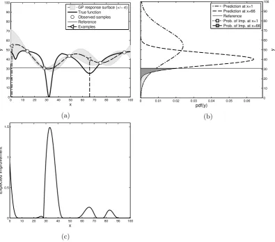
Figure 2.1: Expected improvement illustration for a 1D function. Fig. 2.1a shows an unknown function (bold continuous line) from which 5 samples are observed

(white circles) and are used to fit a GP, whose mean and ±1 standard deviation

confidence interval are represented by the shadowed area with a dashed thick line. Two locations (white triangles) are chosen to illustrate the EI calculation. First, the best observed sample (minimum in this case) is taken as a reference (thin horizontal line), and then for each candidate, the probability of improvement is calculated. For the two selected points for this example, this probability of improvement is shown in Fig. 2.1b as two different overlapping shaded regions. Finally, the expected

improvement (Eq. 2.16) is presented for allxin Fig. 2.1c, where it can be seen that

the EI is maximized for x∗ = 32, which should be considered as the next most

(31)

for static problems [Biermann, Weinert, and Wagner, 2008]. Nevertheless, finding

the global maximum of the EI is a challenging task, since it can be a highly

multi-modal function, so in the next section we propose how to do so in a practical manner.

2.5 Expected improvement maximization

So far, it would seem that all EGO does is to replace the original problem of finding

the global optimum of a (potentially multi-modal) function with a series of problems

of the same kind, since the EI needs to be maximized at each iteration. However,

challenging as it might be to maximize the EI, it is important to keep in mind that

evaluations of the EI improvement function are relatively very cheap as compared

to the original expensive-to-evaluate black-box function, which means that more

traditional methods can be applied.

2.5.1 Expected improvement maximization techniques

Jones, Schonlau, and Welch [1998] originally proposed to use a branch-and-bound

algorithm2to maximize the EI for low dimensional problems, and a limited memory

version of the same algorithm for higher dimension problems. Later, Jones [2001]

proposed to use a multi-start local maximization method where the starting points

are chosen according to an heuristic based on finding midpoints of line segments

connecting pairs of sampled points. This method was first mentioned by Schonlau

[1998] but not explained.

More recent implementations of EGO usually either do not mention the

pro-cedure used to solve this auxiliary problem, or just mention the technique. For

example, Ranjan, Bingham, and Michailidis [2008] uses a genetic algorithm

fine-tuned with a local hill climber, and Kleijnen, Beers, and Nieuwenhuyse [2011] use

either “a space-filling design with candidate points or a global optimizer such as the

genetic algorithm in Forrester, Sobester, and Keane [2008] (p. 78.)”.

Perhaps, this omission is due to the fact that Mockus [1994] stated that

“...there is no need for exact minimization of the risk function. We can use some

simplest methods such as Monte Carlo...”, where risk function refers to a generalized

version of the EI. This statement was repeated then by Schonlau [1998]. In order

2

(32)

to explore whether this statement is true, in the remaining of this section we devise

a simple experiment to test this hypothesis.

2.5.2 Testing the need for good quality EI optimizers

In order to test the impact of finding the global optimum of the EI function, we devise

a simple experimental set-up, where the goal is to maximize a 1-dimensional

multi-modal objective function through sequential optimization starting withλ= 4 initial

random samples, and implementing the EGO algorithm to progressively choose the

next sampling locations.

Two sets of experiments are considered. The first set consists of three

ex-periments using different quality solutions for the EI according to the ranking. To

do this, at each iteration of the EGO algorithm, when the EI shall be maximized,

all the local maxima are found, ranked in decreasing order, and called the kth best

solution (k = 1 being the global optimum). The three experiments in the first set

are fork={1,2,3}.

The second set has only two experiments of which one is the reference

ex-periment (k= 1), and the second one alternates randomly, with equal probability,

betweenk = 1 and k= 2, so as to simulate what would happen with a

maximiza-tion method that finds the global optimum half of the time, while the other half still

returns a good solution (second best local maximum).

Unlike in higher dimensions, finding all the local maxima of a function and

ranking them can be done by exhaustive search using a discretization of the space

whose resolution is fine enough to capture all the characteristics of the EI function,

which for this experiment can safely be assumed to be smooth, given that it is based

on a GP with squared exponential kernel (Eq. 2.4). We consider a local maximum

to be any x for which the associated EI value is strictly greater than both of its

neighboring points in the discretized space. This is why we restrict this experiment

to the 1 dimensional case.

The chosen objective function is

f(x) = max

p=[1...P]

hp wp(x−x∗p)2+ 1

(33)

0 20 40 60 80 100 120 140 160 180 0 0.1 0.2 0.3 0.4 0.5 0.6 0.7 0.8 0.9 1

Number of evaluations

ECDF

k=1 (1e+01) k=2 (1e+01) k=3 (1e+01)

(a) Precision levelf∆= 101

0 20 40 60 80 100 120 140 160 180

0 0.1 0.2 0.3 0.4 0.5 0.6 0.7 0.8 0.9 1

ECDF

k=1 (1e+00) k=2 (1e+00) k=3 (1e+00)

(b) Precision levelf∆= 100

0 20 40 60 80 100 120 140 160 180 200

0 0.1 0.2 0.3 0.4 0.5 0.6 0.7 0.8 0.9 1

ECDF

k=1 (1e−01) k=2 (1e−01) k=3 (1e−01)

(c) Precision levelf∆= 10−1

0 20 40 60 80 100 120 140 160 180 200

0 0.1 0.2 0.3 0.4 0.5 0.6 0.7 0.8 0.9 1

ECDF

k=1 (1e−02) k=2 (1e−02) k=3 (1e−02)

(d) Precision level f∆= 10−2

0 20 40 60 80 100 120 140 160 180 200

0 0.1 0.2 0.3 0.4 0.5 0.6 0.7 0.8 0.9 1

ECDF

k=1 (1e−03) k=2 (1e−03) k=3 (1e−03)

(e) Precision levelf∆= 10−3

0 10 20 30 40 50 60 70

0 0.1 0.2 0.3 0.4 0.5 0.6 0.7 0.8 0.9 1

ECDF k=1 (1e+01) k=1 (1e+00) k=1 (1e−01) k=1 (1e−02) k=1 (1e−03)

[image:33.595.141.501.103.588.2]

(f) All precisions k=1

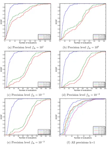
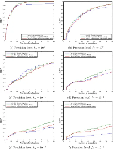
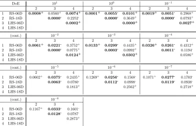
Figure 2.2: Figs. 2.2a through 2.2e compare the performance of three implementa-tions of the EGO algorithm using the ECDF (see Section 2.6.2 for a full explanation

on this error measure). The blue line stands for the implementation using the

global maximum of the EI (k = 1), the green line for the one using the second

best (k = 2), and the red line for the one using the third best local maximum of

the EI (k = 3). Each sub-figure presents the results for different precision levels

(f∆ = {101,100,10−1,10−2,10−3}). For all considered cases, the implementation

where k = 1 largely outperforms the rest. Fig. 2.2f compares the performance of

(34)

0 10 20 30 40 50 60 0 0.1 0.2 0.3 0.4 0.5 0.6 0.7 0.8 0.9 1

ECDF

k=1 (1e+01) k=U[{1,2}] (1e+01)

(a) Precision levelf∆= 101

0 10 20 30 40 50 60 70 80 90 100

0 0.1 0.2 0.3 0.4 0.5 0.6 0.7 0.8 0.9 1

ECDF

k=1 (1e+00) k=U[{1,2}] (1e+00)

(b) Precision level f∆= 100

0 50 100 150

0 0.1 0.2 0.3 0.4 0.5 0.6 0.7 0.8 0.9 1

ECDF

k=1 (1e−01) k=U[{1,2}] (1e−01)

(c) Precision levelf∆= 10−1

0 50 100 150

0 0.1 0.2 0.3 0.4 0.5 0.6 0.7 0.8 0.9 1

ECDF

k=1 (1e−02) k=U[{1,2}] (1e−02)

(d) Precision levelf∆= 10−2

0 50 100 150

0 0.1 0.2 0.3 0.4 0.5 0.6 0.7 0.8 0.9 1

ECDF

k=1 (1e−03) k=U[{1,2}] (1e−03)

[image:34.595.132.511.105.616.2]

(e) Precision levelf∆= 10−3

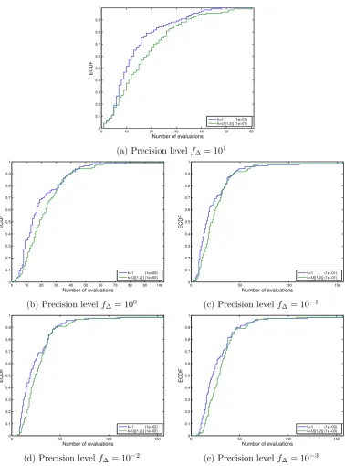
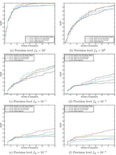
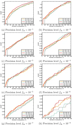
Figure 2.3: ECDF plots (see Section 2.6.2 for a full explanation on this

er-ror measure) comparing the EGO implementation for the reference case (blue

line), where the best peak of the EI is used (k = 1), and the case where

(35)

a combination ofP inverse squared exponentials, each contributing with a peak (or

local maximum) and parametrized by its corresponding width (wp ∈ R+), height

(hp ∈ R+), and peak location (x∗p ∈ R). This function is also used by the

Mov-ing Peaks Benchmark, which is explained in detail in Section 4.3.1 and was first

introduced in Branke [1999].

To ensure the results are statistically significant, R = 20 replications are

run for each number of peaks P ∈ [1. . .6]. We refer to each individual

combina-tion of number of peaks and random realizacombina-tion of parameters as an instance, and

to the aggregate of all replications for all number of peaks as an experiment. At

each instance, the function parameters are drawn from a uniform random

distribu-tion, ensuring that the same instances are presented across different experiments,

as follows:

hp∼U[30,70], (2.19)

wp ∼U[0.01,1],and (2.20)

x∗_p ∼U[0,100]. (2.21)

To evaluate the performance of each implementation, we use a precision

tar-getf_∆∗, defined as the real global maximum of the objective function f∗ minus an

acceptable precision level ∆f. For a given precision level, we can then measure

the number of evaluations it took the optimizer to find the global optimum of the

objective function up to this precision level. By tracking the number of function

evaluations required to achieve a precision target for every instance, we can then

build the empirical cumulative density function (ECDF), which enables for fair and

straightforward comparisons among different optimization methods. Further

expla-nations and justifications for this performance method are given in Section 2.6.2.

Both experiments were run for different precision levels (f∆={101,100,10−1, 10−2,10−3}). The result of the first set of experiments is presented in Figure 2.2 where Figure 2.2a through 2.2e show how the optimizer using the global optimum

of the EI at each iteration (k= 1) largely outperforms those using the second and

third best by having found the global optima at all times in less than 80 function

(36)

oc-0 10 20 30 40 50 60 0

500 1000 1500 2000 2500 3000 3500 4000 4500

Number of observations

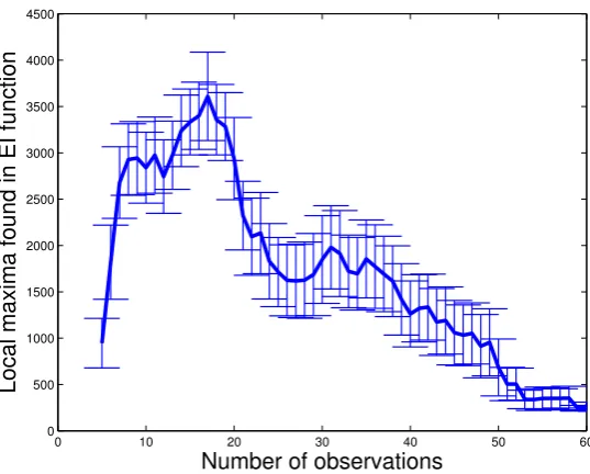
[image:36.595.186.455.107.323.2]

Local maxima found in EI function

Figure 2.4: Number of local maxima found in the EI function with a discretization

grid of step 10−5 throughout the second set of experiments as a function of the

number of observations used to build the response surface. Error bars represent±1

standard error. The decreasing number of local maxima in the EI function towards the end of the experiment is due to a finite size effect.

casions even after 180 function evaluations. Such a large difference occurs because

the optimizer is pushed away from the region where the global maximum is, by not

allowing it to sample ever at the most promising region. This bias is what motivated

the second set of experiments, whose results are presented in Figure 2.3 where the

difference between the reference experiment and the one choosing randomly, with

equal probability, between the best and second best local maximum of the EI, is less

pronounced, yet still noticeable across the tested precision levels.

As a reference, Figure 2.4 shows the number of local maxima found in the

EI function throughout the second set of experiments as a function of the

num-ber of observations used to build the response surface, using a discretization grid

one order of magnitude finer (10−5) than the stopping criterion precision of 10−4.

The decreasing number of local maxima in the EI function towards the end of the

experiment is due to a finite size effect, since simulations converge at different rates.

In an uncontrolled environment and for higher dimensions, it is unlikely that

an optimizer using a local hill climber with multiple starting locations chosen at

(37)

multi-modal nature of the EI function (see Figure 2.6 for an illustration).

These simple experiments demonstrate that the EI maximization is an

im-portant part of the EGO algorithm, and suggest that enough care must be placed

during this task when implementing the EGO algorithm. This is why we devote

Section 2.6 to compare the impact of using different maximization techniques for

the EI in a more elaborated and widely accepted benchmark.

2.6 Selecting an EI maximization technique using the

Black-Box Optimization Benchmark

As shown in Section 2.5.2, it is important to find the global maximum of the EI,

however, allocating too many resources to this task would be time consuming. The

purpose of this section is to determine which optimization technique shall be used

throughout the remainder of this thesis when confronted with the EI maximization

auxiliary problem so as to take the most advantage out of it. To achieve a

thor-ough and fair comparison, we first introduce the black-box optimization benchmark

(BBOB), which provides a comprehensive set of functions and performance

mea-sures to quantify and compare numerical optimization methods. Then, we describe

in detail the algorithms to be compared along with the numeric implementation

details associated to them. Finally, the results of the experiments are presented and

analysed.

2.6.1 The Black-Box Optimization Benchmark

The BBOB provides a well-motivated single-objective set of benchmark functions,

designed to test different aspects of numeric global optimizers along with some

suggested performance measures to facilitate the comparison of different algorithms.

Both, a deterministic (noiseless), and a stochastic (noisy) version of the functions are

proposed by BBOB, but only the former is considered for the experiments described

hereafter. The complete description of the benchmark, including the motivation,

implementation details, and justification for each function in the testbed can be

found in Hansen, Auger, Fincket al. [2010].

(38)

defined for xn ∈ RD(D >2), but they have an artificially chosen global optimum

(f∗) within the compact [−5,5]D, which serves as bounds for the search space. By

providing an instance index to the functions (i∈ {1, ...,15}), different parametriza-tions of the funcparametriza-tions can be instantiated, allowing for the optimizers to be tested on

different versions of the same function so as to provide statistically relevant results.

BBOB considers 24 functions (f₁i, ..., f₂₄i ), all of which are thoroughly explained in

Finck, Hansen, Ros et al. [2010], each contributing with a unique feature so that

valuable information about the tested algorithms can be extracted.

2.6.2 Performance measures

There are typically two methods of measuring the performance of the

implementa-tion of a numeric optimizer.

The first one is to fix a budget (measured in running time, function

evalua-tions, computational time, or any other cost unit), and then measure the quality of

the best outcome returned by the optimizer with respect to the real global optimum.

This seems close to real life needs, where it is often the case that there is a limited

budget to solve a particular problem of which the best possible value is not known3.

The second common option is to fix a desired quality of a solution to be

considered as optimal (target), and then measure the required budget to achieve it,

which requires to know in advance the global optimum of the function.

When solving an unknown problem, the former method is preferred, since

the latter would prove impractical due to the requirement of knowing the solution

in advance. However, the latter provides a quantitative interpretation of the

per-formance by allowing direct comparisons among algorithms. This is better sketched

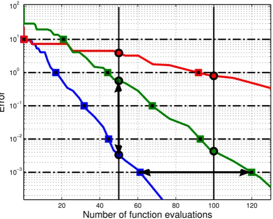
in Figure 2.5, where the error (measured as the difference between the real global

optimum f∗ and the currently best known observation) is plotted as a function of

the number of evaluations for three different algorithms trying to optimize the same

functionf. In this figure, fixing a target means choosing some acceptable level of

error, tracing a horizontal line at such level, and reading in the horizontal axis the

number of function evaluations required to reach the chosen target. For example,

3

(39)

20 40 60 80 100 120

10−3

10−2

10−1

100

101

102

Number of function evaluations

[image:39.595.188.459.110.327.2]

Error

Figure 2.5: Fixed target vs. fixed cost performance measurement.

if we were to compare the performances of the blue and the green optimizers at a

precision level of 10−3 —as shown by the thick horizontal line with arrows—, we

could read that the blue one requires 60 function evaluations to reach it, while the

green one needs 120, concluding that it took twice as many function evaluations to

the green one as compared to the blue one. This provides a quantitative comparison

that can not be achieved with the fixed budget performance measure. For instance,

say we fix the budget at 50 function evaluations (by tracing a vertical line), and

that we want to compare the same two optimizers. We would then read that, for

such a budget, the optimizers achieved an error of 0.003 and 0.5 respectively, which

does not give much insight in the relative performances. So, for benchmarking

pur-poses, since the global optimum is known, the fixed target method is preferred for

performance comparison.

The goal of evaluating the optimizers in a benchmark is to determine which

method should be preferred under unknown conditions. By collecting the resulting

performances after running each optimizer for several instances for each of the

pro-posed functions, we can aggregate the results and build the empirical cumulative

density function (ECDF). The ECDF is built by counting the number of instances

(40)

0 10 20 30 40 50 60 70 80 90 100 0

10 20 30 40 50 60 70 80 90 100

(a) Random multi-start method

0 10 20 30 40 50 60 70 80 90 100

(b) Hyper-box method

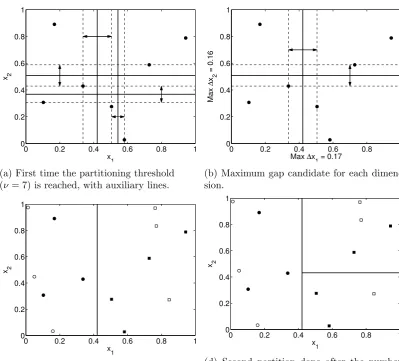
Figure 2.6: Eight random samples in 2D (circles) with dashed lines showing how

the (hyper-)boxes are created. Figure 2.6a shows ζ = (|D|+ 1)D = 81 randomly

allocated starting points (crosses), many of which fall in the same box, leaving other boxes unexplored. Figure 2.6b allocates the same 81 starting points at the center of each (hyper)-box generated by every two neighbor samples, according to the method described in Section 2.6.3.

in a step function that jumps by 1_η at each of the η collected results. The ECDF

is a useful method for aggregating the observed performances because it can be

in-terpreted as the probability for the optimizer of finding the fixed target value. As

its name suggests, the ECDF is built on sample observations, and it is an unbiased

estimator of the fraction of successful runs at each time point (or number of function

evaluations). Moreover, it provides a practical and reliable way of comparing mean

performance of several algorithms. Figure 2.2f is an example of the ECDF used to

display the performance of one numeric optimizer for several precision targets, while

Figure 2.2e illustrates how the ECDF can be used to compare two different numeric

optimizers for a fixed precision target.

2.6.3 EI maximization algorithms comparison

Based on Section 2.5.1, the selected methods to be compared for maximizing the

EI criteria at each iteration of the EGO algorithm are random multi-start local hill

climbers, genetic algorithms, and the hyper-box method, all of which are described

(41)

• The random multi-start with local hill climbers (RMS) method is a stan-dard and generic approach used in global optimization when no information

about the function to be optimized is available [Solis and Wets, 1981]. This

method selects ζ locations at random, uniformly distributed throughout the

domain space, to be used as starting points of local optimizers. Each local

op-timizer implements the Nelder-Mead method (or simplex algorithm) [Nelder

and Mead, 1965]. A disadvantage of this method to maximize the EI is that, as

observations are incorporated toD, new local maxima can be created between

neighboring samples. Jones, Schonlau, and Welch [1998] explicitly

discour-age the use of this method for the same reason. Even with a large number of

starting points for the local hill climbers, the probability of leaving unexplored

at least one hyper-box (defined by a pair of neighboring samples), increases

exponentially with the cardinality ofD, as is illustrated in Figure 2.6a.

• The hyper-box multi-start with local hill climbers (HB) method exploits the

structure of the EI function by selecting the starting points at the center of

each hyper box created by every pair of neighbor samples, which requiresζ =

(|D|+ 1)D starting points. Their initial step size is chosen such that each local hill climber, implementing the Nelder-Mead method as well, does not leave

its corresponding hyper-box in the first step, forcing it to explore the locality.

This method is still a heuristic and does not guarantee to find the global

maximum of the EI, but it shows better performance than random multi-start

locations. An illustration of the HB method for a 2 dimensional problem is

shown in Figure 2.6b. The HB sampling method is loosely based on a method

originally proposed by Jones [2001], which is shortly sketched in the Appendix,

however, such a method is based on finding the midpoints of line segments

connecting pairs of sampled points, and then applying a clustering method,

while the HB method generates a starting point in between any possible pair

of samples.

• The genetic algorithm (GA) method starts by generating an initial set of

so-lutions called population, which are selected uniformly at random from the

(42)

objec-tive function (EI in this case), and the individuals of this initial population

are ranked according to their performance (or fitness). The algorithm then

creates a sequence of new populations, which are called generations. At each

step, the new population is created based on the population of the

previ-ous generation by creating three different types of children. The first type is

elite based, and is performed simply by selecting the 2 best individuals of the

previous population. The second type, generated by crossover, accounts for

80% of the population and is the result of randomly selecting pairs of

par-ents out of the entire pool of individuals from the previous generation, with

a distribution reflecting the individual’s fitness, and combining their vector

components (genes) through a weighted average with random weights. This

procedure is known as scattered crossover. The final type of children are

gen-erated by mutation, which accounts for the remainder of the population. This

is done by randomly selecting single parents from the same distribution as in

the crossover operation, and adding Gaussian noise to them with zero mean

and and standard deviation 1. The whole process is then repeated for several

generations.

In order to make the number of EI function evaluations simple to compare,

the population size and the number of generations for which the process is

repeated are kept constant for the experiments described in this chapter. The

number of generations and the population size are calculated so that the total

number of EI function evaluations used by the RMS method can be attained.

From the experiments performed, it was calculated that 400 generations, each

of 400 individuals, satisfy this requirement. Nevertheless, for further chapters,

we propose to dynamically adjust these parameters depending on the size

of the problem to be solved. So, in Chapter 3, instead of using a constant

size for the population and the number of generations, these parameters are

set tolυ√N Dm, where the user defined EI maximization budget constantυ

is inferred from the data collected during the experiments performed at the

current stage (comparison between HB, RMS, and GA).

Since the real interest is not in maximizing the auxiliary problem, but rather

Efficient sequential sampling for global optimization in static and dynamic environments

University of Warwick institutional repository: http://go.warwick.ac.uk/wrap

A Thesis Submitted for the Degree of PhD at the University of Warwick

http://go.warwick.ac.uk/wrap/62123

This thesis is made available online and is protected by original copyright.

Please scroll down to view the document itself.

Efficient sequential sampling for global optimization

in static and dynamic environments

Sergio Morales Enciso

Complexity Sciences and Operational Research

Contents

List of Tables

List of Figures

Acknowledgments

Declarations

Abstract

List of Abbreviations

Chapter 1

Introduction

Chapter 2

Global optimization of

expensive-to-evaluate black-box

functions

2.1

Global optimization of expensive-to-evaluate

black-box functions

2.2

Initial design of experiments for sequential

sam-pling optimization

2.3

Gaussian processes as response surfaces

for optimization

2.4

Sequential optimization

2.5

Expected improvement maximization

2.6

Selecting an EI maximization technique using the

Black-Box Optimization Benchmark