What is the probability that a random integral quadratic form in n variables has an integral zero?

(1)

http://wrap.warwick.ac.uk

Original citation:

Bhargava, Manjul, Cremona, John E., Fisher, Tom, Jones, Nick G. and Keating,

Jonathan P.. (2015) What is the probability that a random integral quadratic form inn

variables has an integral zero? International Mathematics Research Notices . rnv251.

10.1093/imrn/rnv251

Permanent WRAP url:

http://wrap.warwick.ac.uk/75680

Copyright and reuse:

The Warwick Research Archive Portal (WRAP) makes this work of researchers of the

University of Warwick available open access under the following conditions.

This article is made available under the Creative Commons Attribution 4.0 International

license (CC BY 4.0) and may be reused according to the conditions of the license. For

more details see:

http://creativecommons.org/licenses/by/4.0/

A note on versions:

The version presented in WRAP is the published version, or, version of record, and may

be cited as it appears here.

(2)

M. Bhargava et al. (2015) “Random Integral Quadratic Forms,” International Mathematics Research Notices, rnv251, 21 pages. doi:10.1093/imrn/rnv251

What is the Probability that a Random Integral Quadratic

Form in

n

Variables has an Integral Zero?

Manjul Bhargava

1

, John E. Cremona

2

, Tom Fisher

3

,

Nick G. Jones

4

, and Jonathan P. Keating

4

1

_{Department of Mathematics, Princeton University, Princeton, NJ 08544,}

USA,

2

Mathematics Institute, Zeeman Building, University of Warwick,

Coventry CV4 7AL, UK,

3

DPMMS, Centre for Mathematical Sciences,

Wilberforce Road, Cambridge CB3 0WB, UK, and

4

School of

Mathematics, University of Bristol, Bristol BS8 1TW, UK

Correspondence to be sent to: e-mail: [email protected]

We show that the density of quadratic forms innvariables overZpthat are isotropic is a

rational function ofp, where the rational function is independent ofp, and we determine this rational function explicitly. When real quadratic forms innvariables are distributed according to the Gaussian Orthogonal Ensemble (GOE) of random matrix theory, we determine explicitly the probability that a random such real quadratic form is isotropic (i.e., indefinite). As a consequence, for eachn, we determine an exact expression for the probability that a random integral quadratic form innvariables is isotropic (i.e., has a nontrivial zero overZ), when these integral quadratic forms are chosen according to the GOE distribution. In particular, we find an exact expression for the probability that a random integral quaternary quadratic form is isotropic; numerically, this probability of isotropy is approximately 98.3%.

Received March 20 2015; Revised July 2, 2015; Accepted July 27, 2015 c

The Author(s) 2015. Published by Oxford University Press.

This is an Open Access article distributed under the terms of the Creative Commons Attribution License (http://creativecommons.org/licenses/by/4.0/), which permits unrestricted reuse, distribution, and reproduction in any medium, provided the original work is properly cited.

at University of Warwick on January 14, 2016

http://imrn.oxfordjournals.org/

(3)

1 Introduction

An integral quadratic formQinnvariables is a homogeneous quadratic polynomial

Q(x1,x2, . . . ,xn)=

1≤i≤j≤n

ci jxixj, (1)

where all coefficients ci j lie in Z. The quadratic form Q is said to be isotropic if

it represents 0, that is, if there exists a nonzero n-tuple (k1, . . . ,kn)∈Zn such that Q(k1, . . . ,kn)=0. We wish to consider the question: what is the probability that a random

integral quadratic form innvariables is isotropic?

In this paper, we give a complete answer to this question for all n, when inte-gral quadratic forms innvariables are chosen according to the Gaussian Orthogonal Ensemble (GOE) of random matrix theory [1]. In particular, in the most interesting case

n=4, we show that the probability that a random integral quaternary quadratic form is isotropic is given by

1 2+

√

2 8 +

1 π

p

1− p

3

4(p+1)2₍_p4₊_p3₊_p2₊_p₊₁₎

≈98.25845607%. (2)

More precisely, let D be a piecewise smooth rapidly decaying function on the vector space Rn(n+1)/2 _{of real quadratic forms in} _n_{variables (i.e.,} _D₍_x₎_{and all its}

par-tial derivatives areo(|x|−N₎_{for all}_N_>_{0), and assume that}

QD(Q)dQ=1; we call such

a function D a nice distribution on the space of realn-ary quadratic forms. Then we define the probability, with respect to the distribution D, that a random integraln-ary quadratic formQhas a property P by

lim

X→∞

Qintegral ,with propertyP D(Q/X)

QintegralD(Q/X)

, (3)

if the limit exists. Letρ_nD denote the probability with respect to the distributionDthat a random integral quadratic form innvariables is isotropic. If D=GOE is the distribu-tion on the space ofn×nsymmetric matrices given by _√1

2(A+A

t₎_{, where each entry of}

the matrix Ais an identical and independently distributed real Gaussian—that is, the GOE—then we useρn:=ρnGOEto denote the probability, with respect to the GOE

distri-bution, that a randomn-ary quadratic form overZis isotropic.

We wish to explicitly determine the probabilityρnthat a randomn-ary quadratic

form overZ, with respect to the GOE distribution, is isotropic, that is, has a nontrivial zero over Z. To accomplish this, we first recall the Hasse–Minkowski Theorem, which

(4)

states that a quadratic form overZis isotropic if and only if it is isotropic overZpfor

all pand overR. For any distributionDas above, letρD

n(p)denote the probability that a

random integral quadratic form, with respect to the distributionD, is isotropic overZp,

and letρD

n(∞)denote the probability that it is isotropic overR(i.e., is indefinite). Then it

is not hard to show (for the details, see Section2) thatρn(p)=ρnD(p)is independent ofD,

and is simply given by the probability that a randomn-ary quadratic form overZp, with

respect to the usual additive measure onZnp(n+1)/2, is isotropic overZp. Moreover, we will

also show in Section2that the probabilityρD

n(∞)that a randomintegralquadratic form

is isotropic overRis equal to the probability that a randomreal quadratic form (with respect to the same distributionD) is indefinite.

For any distribution Das above, the following theorem can be proved using the work of Poonen and Voloch [11] together with the Hasse–Minkowski Theorem:

Theorem 1.1. The probability ρ_nD that a random (with respect to the distribution D) integral quadratic form in nvariables is isotropic is given by the product of the local probabilities:

ρD n =ρ

D n(∞)

p

ρn(p). (4)

See Section2for details. Hence, to determineρD

n, it suffices to determineρnD(∞)

andρn(p)for all p.

We treat first the probabilityρn(p)that a randomn-ary quadratic form overZp

is isotropic. Our main result here is that, for each n, the quantity ρn(p) is given by a

fixed rational function in pthat is independent of p(this even includes the case p=2), and we determine these rational functions explicitly. Specifically, we prove the following theorem:

Theorem 1.2. Letρn(p)denote the probability that a quadratic form innvariables over Zpis isotropic. Then

ρ1(p)=0, ρ2(p)=

1

2, ρ3(p)=1−

p

2(p+1)2,

ρ4(p)=1−

p3

4(p+1)2₍_p4₊_p3₊_p2₊_p₊₁₎,

andρn(p)=1 for alln≥5.

Our method of proof for Theorem1.2is uniform inn, and relies on establishing certain recursive formulae for densities of local solubility for certain subsets ofn-ary

(5)

quadratic forms defined by their behavior modulo powers ofp. In particular, we obtain a new recursive proof of the well-known fact that everyn-ary quadratic form overQpis

isotropic whenn≥5. See Section3for details.

We turn next to the probabilityρn(∞)=ρnGOE(∞)that a realn-ary quadratic form

is isotropic overR. Closed form expressions forρn(∞)for n≤3 were first given by

Bel-tran [5, (7)]; it is also known that 1−ρn(∞)decays like e−n 2₍_{log 3}_)/₄

asn→ ∞(see [2,3]). In Section4, we show how to obtain an exact formula forρn(∞)for any givenn.

More precisely, using the de Bruijn identity [4] for calculating certain determinan-tal integrals, we express ρn(∞) as the Pfaffian of an explicit n×n matrix, where n:=2n/2, whose entries are given in terms of values of the gamma and incomplete beta functions at integers and half-integers. Indeed, let Γ denote the usual gamma function Γ (s)=₀∞xs−1_e−x_d_x _{and let} _β

t denote the usual incomplete beta function

βt(i,j)=

t

0x

i−1₍₁₋_x₎j−1_d_x_{. Then we have the following theorem giving expressions}

forρn(∞):

Theorem 1.3. Letn≥1 be any integer, and definen:=2n/2. When realn-ary quadratic forms are chosen according to then-dimensional GOE, the probability of isotropy over

Ris given by

ρn(∞)=1−

Pf(A)

2(n−1)(n+4)/4 n

m=1Γ (m2)

, (5)

whereAis then×nskew-symmetric matrix whose(i,j)-entryai jis given fori<jby

ai j=

⎧ ⎪ ⎪ ⎪ ⎨ ⎪ ⎪ ⎪ ⎩

2i+j−2_Γ

i+ j

2 β12

i

2,

j

2

−β1 2

j

2,

i

2

if i<j≤n,

2i−1_Γ

i

2

if i<j=n+1.

(6)

(Note that the second case in(6)arises only whennis odd.)

Theorem1.3allows one to calculateρn(∞)exactly in closed form for any givenn.

In particular, it follows from the Pfaffian representation in Theorem1.3thatρn(∞)is a

polynomial inπ−1_{of degree at most}n+1

4 with coefficients inQ( √

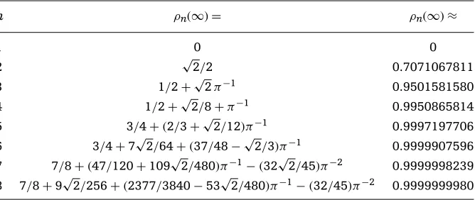
2)(see Remark4.1). In Table1, we give the resulting formulae forρn(∞)for alln≤8, and also provide numerical

approximations. (For anyn>8, we haveρn(∞)≈1 to more than 10 decimal places!)

Combining Theorems1.1–1.3, we finally obtain the following theorem giving the probabilityρnthat a random integral quadratic form innvariables has an integral zero.

(6)

[image:6.536.106.440.83.224.2]

Table 1. Probabilityρn(∞)that a randomn-ary quadratic form overRfrom the GOE distribution is isotropic, forn≤8

n ρn(∞)= ρn(∞)≈

1 0 0

2 √2/2 0.7071067811

3 1/2+√2π−1 0.9501581580 4 1/2+√2/8+π−1 0.9950865814 5 3/4+(2/3+√2/12)π−1 0.9997197706 6 3/4+7√2/64+(37/48−√2/3)π−1 0.9999907596 7 7/8+(47/120+109√2/480)π−1−(32√2/45)π−2 0.9999998239 8 7/8+9√2/256+(2377/3840−53√2/480)π−1₋₍₃₂_/₄₅_)π−2 _0.9999999980

Theorem 1.4. Let Dbe any nice (i.e., piecewise smooth and rapidly decaying) distribu-tion. Then the probabilityρ_nDthat a random integral quadratic form innvariables with respect to the distributionDis isotropic is given by

ρD n =

⎧ ⎪ ⎪ ⎪ ⎪ ⎪ ⎪ ⎪ ⎨ ⎪ ⎪ ⎪ ⎪ ⎪ ⎪ ⎪ ⎩

0 ifn≤3;

ρD 4(∞)

p

1− p

3

4(p+1)2(_p4+_p3+_p2+_p+1)

ifn=4;

ρD

n(∞) ifn≥5.

If D=GOE is the GOE distribution, then the quantitiesρn(∞)=ρnD(∞)are as given in

Theorem1.3.

In particular, whenD=GOE, we haveρn=0 forn=1,2, and 3, while forn=4 we

obtain the expression (2) forρ4. Forn≥5, we haveρn=ρn(∞), and so the values ofρnare

as given by Theorem1.3. Theorem1.4shows thatn=4 is in a sense the most interesting case, as all places play a nontrivial role in the final answer.

It is also interesting to compare how the probabilities change if instead of the GOE we use the uniform distribution U on quadratic forms, where each coefficient of the quadratic form is chosen uniformly in the interval −1

2, 1 2

. While the quantities ρU

n(∞)can easily be expressed as explicit definite integrals, it seems unlikely that they

can be evaluated in compact and closed form for generalnin this case. Using numer-ical integration, or a Monte Carlo approximation, we can compute ρU

n(∞)≈0, 0.627,

0.901, 0.982, 0.998, and>0.999 forn=1, 2, 3, 4, 5, and 6, respectively. It is known that 1−ρU

n(∞)decays faster than e−cnfor some constant c>0. This is a particular case of

[1, Theorem. 2.3.5] which applies to a large class of random matrices including both

(7)

[image:7.536.88.445.96.227.2]

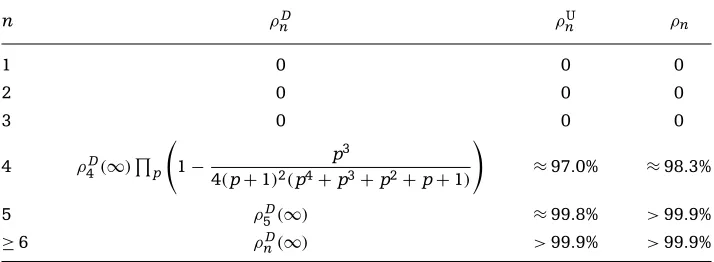
Table 2. Probability that a random integral quadratic form in n variables is isotropic, for a general distributionD, for the uniform distribution, and for the GOE distribution

n ρ_nD ρ_nU ρn

1 0 0 0

2 0 0 0

3 0 0 0

4 ρD 4(∞) p

1− p

3

4(p+1)2₍_p4₊_p3₊_p2₊_p₊₁₎

≈97.0% ≈98.3%

5 ρD

5(∞) ≈99.8% >99.9%

≥6 ρD

n(∞) >99.9% >99.9%

those with uniform entries and the GOE. The actual rate of decay for the GOE is faster as noted above, and we expect this also in the uniform case.

In particular, we have ρ₄U=ρ₄U(∞) _pρ4(p)≈97.0%, which is slightly smaller

than the GOE probabilityρGOE₄ ≈98.3%. We summarize the values of ρD

n, and provide

numerical values in the cases of the uniform and GOE distributions, in Table2.

Let Nn(X)denote the number of integraln-ary quadratic forms that are isotropic overZ whose coefficients are less than X in absolute value. Since the probabilities of isotropy are equal to 0 forn≤3, the question arises as to howNn(X)grows in these cases

asX→ ∞. Forn=1, we have triviallyN1(X)=1 for anyX>0. Forn=2, it was shown by

D ¨orge [6] and Kuba [10] that X2_log_X_N

2(X)X2logX, and this was recently refined

to an exact asymptotic formula, N2(X)∼c2X2logXfor an explicit positive constantc2,

by Dubickas [7]. For n=3, it was shown by Serre [13] that N3(X)=O(X6/

logX), who also conjectured thatN3(X) >E X6/

logXfor some positive constantE; this conjecture was recently resolved by Hooley [9]. In conjunction with these results forn≤3, the result of Theorem1.4determines the rates of growth of Nn(X)for alln≥1, and indeed proves the existence of main terms in the asymptotics ofNn(X)for alln=3. (Whether N3(X)∼ c3X6/

logXfor some positive constantc3remains an open question.)

This paper is organized as follows. In Section2, we prove the product formula in Theorem1.1. The theorem is known in the case of the uniform distribution U (or indeed any uniform distribution supported on a box) for anyn≥4 by the work of Poonen and Voloch [11], which in turn depends on the Ekedahl sieve [8]. To complete the proof of Theorem1.1, we first prove directly that both sides of (4) are equal to 0 for n≤3. For

n≥4, we prove that (4) is true for a general nice distributionDby approximatingDby a finite weighted average of uniform box distributions, where the result is already known.

(8)

The condition that Dis rapidly decreasing (as in the case of D=GOE) plays a key role in the proof; indeed, we show how counterexamples to (4) can be constructed when this condition does not hold.

In Section 3, we then prove Theorem 1.2, that is, we determine for eachnthe exact p-adic density ofn-ary quadratic forms overZpthat are isotropic. The outline of

the proof is as follows. First, we note that a quadratic form innvariables defined overZp

can be anisotropic only if its reduction modulophas either two conjugate linear factors overFp2 or a repeated linear factor over F_p. We first compute the probability of each

of these cases occurring, which is elementary. We then determine the probabilities of isotropy in each of these two cases by developing certain recursive formulae for these probabilities, in terms of other suitable quantities, which allow us to solve and obtain exact algebraic expressions for these probabilities for each value ofn. We note that our general argument shows in particular that quadratic forms inn≥5 variables over Qp

are always isotropic, thus yielding a new recursive proof of this well-known fact. Finally, we prove Theorem 1.3in Section4, that is, we determine for eachnthe probability that a random realn-ary quadratic form from the GOE distribution is indef-inite. We accomplish this by first expressing, as a certain determinantal integral, the probability that ann×nsymmetric matrix from the GOE distribution has all positive eigenvalues. We then show how this determinantal integral can be evaluated using the de Bruijn identity [4], allowing us to obtain an expression for the probability of positive definiteness in terms of the Pfaffian of an explicit skew-symmetric matrixA, as given in Theorem1.3.

We end this introduction by remarking that the analogues of Theorems 1.2

and1.4also hold over a general local or global field, respectively. Here, we define global densities of quadrics as in [11, Section 4]; more general densities with respect to “nice distributions” could also be defined in an analogous manner. Indeed, the analogue of Theorem1.1holds (with the identical proof), where the product on the right-hand side of (4) should be taken over all finite and infinite places of the number field (the densities at the complex places are all equal to 1, since all quadratic forms overCare isotropic). Theorem1.2also holds over any finite extension ofQp, with the same proof, provided

that when making substitutions in the proofs we replace pby a uniformiser, and when computing probabilities we replacepby the order of the residue field.

2 The Local Product Formula: Proof of Theorem 1.1

LetDbe any nice (piecewise smooth and rapidly decaying) distribution. Our aim in this section is to prove the following three assertions from the introduction:

(9)

(a) ρ_nD(p)is equal to the probability ρn(p)that a random n-ary quadratic form

over Zp, with respect to the usual additive measure on Znp(n+1)/2, is isotropic

overZp;

(b) ρD

n(∞)is equal to the probability that a randomn-ary quadratic form overR,

with respect to the distribution D, is indefinite; and (c) ρD

n =ρnD(∞) pρn(p)(i.e., Theorem1.1holds).

Items (a) and (b) are trivial in the case that D=U is the uniform distribu-tion, or more generally when D is any distribution U(a,b) that is constant on a box [a,b] :=[a1,b1]× · · · ×[an(n+1)/2,bn(n+1)/2] and 0 outside this box; herea=(a1, . . . ,an(n+1)/2)

andb=(b1, . . . ,bn(n+1)/2)are vectors inRn(n+1)/2such thatai<bifor alli.

Meanwhile, Theorem 1.1 for n≥4, in the case that D is the uniform distribu-tion U, follows from the work of Poonen and Voloch [11, Theorem 3.6] (which establishes the product formula for the probability that an integral quadratic form with respect to the distribution D is locally soluble), together with the Hasse–Minkowski Theorem (which states that a quadratic form is isotropic if and only if it is locally soluble). In fact, the proof of [11, Theorem 3.6] (which in turn relies on Ekedahl’s sieve [8]) immedi-ately adapts to the case whereD=U(a,b)without essential change.

To show that Theorem 1.1 holds also when D=U(a,b) and n≤3, it suffices to prove that in this case both sides of (4) are equal to 0. To see this, we may use Theorem1.2, which does not rely on the results of this section, and which states that the probability that a randomn-ary quadratic form overZpis isotropic is equal toρn(p)=0,

1/2, or 1−p/(2(p+1)2)forn=1, 2, or 3, respectively. This immediately implies that the right-hand side of (4) is zero. To see that the left-hand side of (4) is zero, we note that if a quadratic form overZis isotropic, then it must be isotropic overZpfor all p(the easy

direction of the Hasse–Minkowski Theorem). By the Chinese Remainder Theorem, the (limsup of the) probabilityρD

n that a random integraln-ary quadratic form is isotropic

with respect to the distributionD=U(a,b)is at most

p<Y

ρn(p)

for anyY>0. LettingYnow tend to infinity shows thatρD

n =0 forn=1, 2, or 3, that is,

the left-hand side of (4) is also zero.

Thus we have established items (a)–(c), for alln, in the case that D=U(a,b)is a constant distribution supported on a box [a,b]. Clearly, (a)–(c) then must hold also for any finite weighted average of such box distributions U(·,·).

(10)

To show that (a)–(c) hold for general nice distributions D, we make use of the following elementary lemma regarding integration of rapidly decaying functions.

Lemma 2.1. Let f be any piecewise smooth rapidly decaying function onRm_{. Then}

f(y)dy= lim

X→∞

1

Xm

y∈Zm

f(y/X). (7)

Proof. For any N>0, let fN(y)be equal to f(y)if|y| ≤N, and 0 otherwise. Then fN is

piecewise smooth with bounded support, and so is Riemann integrable. Thus we have

fN(y)dy= lim

X→∞

1

Xm

y∈Zm

fN(y/X). (8)

Since f is rapidly decreasing, for any ε >0 we may choose N large enough so that

|y|>N|f(y)|dy< εand(1/Xm)

y∈Zm_,_|_y_/_X_|_>_N|f(y/X)|< εfor anyX≥1. For this value ofN, the left-hand side of (8) is withinεof the left-hand side of (7), while for eachX≥1, the expression in the limit on the right-hand side of (8) is within ε of the expression in the limit on the right-hand side of (7). Since we have equality in (8), we conclude that the left-hand side of (7) is within 2ε of both the lim infX→∞ and the lim supX→∞ of the

expression in the limit of the right-hand side of (7). Sinceεis arbitrarily small, we have

proven (7).

Note that Lemma2.1does not necessarily hold if we drop the condition that f

is rapidly decaying. For example, if f is the characteristic function of a finite-volume region having a cusp going off to infinity containing a rational line through the origin (and thus infinitely many lattice points on that line), then the left-hand side of (7) is finite while the expression in the limit on the right-hand side of (7) is infinite for any rational value ofX.

Lemma2.1implies in particular that

lim

X→∞

1

Xn(n+1)/2

Qintegral

D(Q/X)=1 (9)

for any nice distributionD.

Now any piecewise smooth rapidly decaying function can be approximated arbi-trarily well by a finite linear combination of characteristic functions of boxes. Let D

be a nice distribution. For anyε >0, we may find a nice distribution D_εthat is a finite

(11)

weighted average of box distributions U(·,·), such that

|D(y)−D_ε(y)|dy< ε. (10)

By Lemma2.1, we then have

lim

X→∞

1

Xn(n+1)/2

Qintegral

|D(Q/X)−D_ε(Q/X)|< ε. (11)

To show thatρ_nD(p)=ρn(p), we note that

ρn(p)=ρnDε(p)= lim X→∞

Qintegral,isotropic/ZpDε(Q/X)

QintegralDε(Q/X)

(12)

= lim

X→∞

Qintegral,isotropic/ZpDε(Q/X)

Xn(n+1)/2 (13)

= lim

X→∞

Qintegral,isotropic/ZpD(Q/X)+E(X, ε)

Xn(n+1)/2 (14)

= lim

X→∞

Qintegral,isotropic/ZpD(Q/X)+E(X, ε)

QintegralD(Q/X)

, (15)

where for sufficiently largeXwe have|E(X, ε)|< εXn(n+1)/2_{by (}₁₁_{); here the first equality}

follows because D_ε is a finite weighted average of box distributions U(·,·), the second equality follows from the definition (3), and the third and fifth equalities follow from (9). Letting ε tend to 0 in (15) now yields ρn(p)=ρnD(p), proving item (a) for general nice

distributionsD.

Analogously, we have

Qisotropic/R

D_ε(Q)dQ=ρDε

n (∞)=_Xlim_→∞

Qintegral ,isotropic/RDε(Q/X)

QintegralDε(Q/X)

(16)

= lim

X→∞

Qintegral,isotropic/RD(Q/X)+E(X, ε) QintegralD(Q/X)

, (17)

where again for sufficiently large X we have |E(X, ε)|< εXn(n+1)/2_{. By (}₁₀_{), the}

left-most expression in (16) approaches_Q_isotropic_/_RD(Q)dQasε→0, while expression (17) approachesρD

n(∞)by definition (3). This thus proves item (b) for general nice

distribu-tions. In particular, we have also proven that

lim

ε→0ρ Dε

n (∞)=ρnD(∞). (18)

(12)

Finally, we have in a similar manner:

ρD_ε n (∞)

p

ρn(p)=ρnDε=_Xlim_→∞

Qintegral ,isotropic/ZDε(Q/X)

QintegralDε(Q/X)

(19)

= lim

X→∞

Qintegral,isotropic/ZD(Q/X)+E(X, ε)

QintegralD(Q/X)

, (20)

where again for sufficiently large X we have|E(X, ε)|< εXn(n+1)/2_{. By (}₁₈_{), the leftmost}

expression in (19) approachesρD

n(∞) pρn(p)asε→0, while expression (20) approaches

ρD

n by definition. We have proven also item (c) for general nice distributions, as desired.

3 The Density ofn-ary Quadratic Forms OverZpthat are Isotropic: Proof of Theorem1.2

3.1 Preliminaries onn-ary quadratic forms overZp

Fix a prime p. For any free Zp-module V of finite rank, there is a unique additive p-adic Haar measure μV on V which we always normalize so that μV(V)=1. All

den-sities/probabilities are computed with respect to this measure. In this section, we take

V=Vnto be then(n+1)/2-dimensionalZp-module ofn-ary quadratic forms overZp. We

then work out the density ρn(p) (i.e., measure with respect to μV) of the set of n-ary

quadratic forms overZpthat are isotropic.

We start by observing that a primitive n-ary quadratic form over Zp can be

anisotropic only if, either: (I) the reduction modulo pfactors into two conjugate lin-ear factors defined over a quadratic extension ofFpor (II) the reduction modulo pis a

constant times the square of a linear form overFp. For if the reduced form has rank≥3,

then, after setting some variables to zero we obtain a smooth conic. But a conic over a finite field always has a rational point (see, e.g., [12, Chapter I, Corollary 2]); this lifts to aQp-point by Hensel’s Lemma. Note that if p=2, this argument is still valid, provided

that we define the rank correctly, that is, it is not the rank of the corresponding symmet-ric matrix, but rather the codimension of the singular locus in the ambient projective space.

Let ξ₁(n) andξ₂(n) be the probabilities of Cases I and II, that is, the densities of these two types of quadratic forms inVn. Then

ξ(n)

0 =1−ξ( n)

1 −ξ( n)

2 −

1

pn(n+1)/2

(13)

is the probability that a form is primitive, but not in Case I or Case II. Letα₁(n) (respec-tively, α(₂n)) be the probability of isotropy for quadratic forms in Case I (respectively, Case II). Then

ρn(p)=ξ0(n)+ξ( n) 1 α(

n) 1 +ξ(

n) 2 α(

n) 2 +

1

pn(n+1)/2ρn(p),

implying that

ρn(p)=

pn(n+1)/2 pn(n+1)/2−₁

ξ(n)

0 +ξ( n)

1 α( n)

1 +ξ( n)

2 α( n)

2

. (21)

3.2 Some counting over finite fields

Letη(₁n)(respectively,η(₂n)) be the probability that a quadratic form is in Case I (respec-tively, Case II) given the “point condition” that the coefficient ofx2

1 is a unit. Similarly,

letν₁(n) be the probability that a quadratic form is in Case I given the “line condition” that the binary quadratic formQ(x1,x2,0, . . . ,0)is irreducible modulo p. Note that it is

impossible to be in Case II given the line condition, but we may also defineν₂(n)=0. Set η(n)

0 =1−η( n)

1 −η( n)

2 andν( n)

0 =1−ν( n)

1 −ν( n)

2 =1−ν( n)

1 . The values ofξ( n)

j ,η( n)

j , and ν( n)

j are

given by the following easy lemma.

Lemma 3.1. The probabilities that a random quadratic form overZpis in Case I or Case

II are as follows:

• Case I (all; relative to point condition; relative to line condition)

ξ(n)

1 =

(pn₋₁₎₍_pn₋_p₎

2(p+1)pn(n+1)/2; η

(n)

1 =

pn−1₋₁

2pn(n−1)/2; ν

(n)

1 =

1

p(n−1)(n−2)/2.

• Case II (all; relative to point condition; relative to line condition)

ξ(n)

2 =

pn₋₁ pn(n+1)/2; η

(n)

2 =

1

pn(n−1)/2; ν

(n)

2 =0.

Proof. Case I: there are(p2n₋₁_)/(_p2₋₁₎_{linear forms over}_F

p2 up to scaling;

subtract-ing the(pn₋₁_)/(_p₋₁₎_{which are defined over}_F

p, dividing by 2 to account for conjugate

pairs and then multiplying byp−1 for scaling gives (pn−₂₍1_p)(₊p₁n₎−p) Case I forms, and hence the value ofξ₁(n).

Similarly, the number of Case I quadratic forms satisfying the point condition is (p2(n−1)₋_pn−1₎₍_p₋₁_)/_{2. Dividing by the probability 1}₋₁_/_p _{of the point condition}

holding gives pn₍_pn−1₋₁_)/_{2 and hence the value of}_η(n)

1 .

(14)

Lastly, the number of Case I quadratic forms satisfying the line condition is p2n−3₍_p₋₁₎2_/_{2; dividing by the probability} _ξ(2)

1 of the line condition holding gives p2n−1_{, and hence the value of}_ν(n)

1 .

Case II is similar and easier: the number of Case II quadratic forms is pn₋_{1, of}

whichpn₋_pn−1_{satisfy the point condition and none satisfy the line condition; the given}

formulae follow.

3.3 Recursive formulae

We now outline our strategy for computing the densities ρn(p)using (21), by

evaluat-ingα(_jn)for j=1,2. If a quadratic form is in Case I, then we may make a linear change of variables (using a change of coordinate matrix in GLn(Zp), which preserves density),

transforming it so that its reduction is an irreducible binary form in only two variables. Now isotropy forces the values of those variables, in any primitive vector giving a zero, to be multiples ofp; so we may scale those variables by pand divide the form byp. Sim-ilarly, if a form is in Case II, then we transform it so that its reduction is the square of a single variable, then scale that variable and divide out. After carrying out this process once, we again divide into cases and repeat the procedure, which leads us back to an earlier situation but with either the line or point conditions, which we need to allow for. All these transformations clearly preserve the property of isotropy.

To make this precise, we introduce some extra notation for the probability of isotropy for quadratic forms which are in Case I or Case II after the initial trans-formation: let β₁(n) (respectively, β₂(n)) be the probability of isotropy given we are in Case I (respectively, Case II) after one step when the original quadratic form was in Case I, and similarly γ₁(n) (respectively, γ₂(n)) the probability of isotropy given we are in Case I (respectively, Case II) after one step when the original quadratic form was in Case II.

Lemma 3.2.

1. α(₁2)=0, and forn≥3,

α(n)

1 =ξ( n−2)

0 +ξ( n−2)

1 β( n)

1 +ξ( n−2)

2 β( n)

2 +

1

p(n−1)(n−2)/2

ν(n)

0 +ν( n)

1 α( n)

1 +ν( n)

2 α( n)

2

.

2. α(₂1)=0, and forn≥2,

α(n)

2 =ξ( n−1)

0 +ξ( n−1)

1 γ( n)

1 +ξ( n−1)

2 γ( n)

2 +

1

pn(n−1)/2

η(n)

0 +η( n)

1 α( n)

1 +η( n)

2 α( n)

2

.

(15)

Proof. We have α(₁2)=0 since a binary quadratic form that is irreducible over Fp is

anisotropic. Now assume thatn≥3, and (for Case I) Q(x1, . . . ,xn) (mod p)has two

con-jugate linear factors. Without loss of generality, the reduction modulo pis a binary quadratic form inx1andx2. Now any primitive vector giving a zero of Qmust have its

first two coordinates divisible by p, so replace Q(x1, . . . ,xn)by 1_pQ(px1,px2,x3, . . . ,xn).

The reduction modulo pis now a quadratic form inx3, . . . ,xn. If the newQis identically

zero modulo p, then, after dividing it by p, we obtain a new integral form that lands in Cases I and II with probabilitiesν₁(n) andν₂(n), respectively, since it satisfies the line condition; otherwise, we divide into cases as before, with the probabilities of being in each case given byξ(_jn−2).

The result for α₂(n) is proved similarly: without loss of generality the reduction modulo pis a quadratic form inx1only, we replace Q(x1, . . . ,xn)by 1_pQ(px1,x2, . . . ,xn),

whose reduction modulo pis a quadratic form in x2, . . . ,xn. If the new Qis identically

zero modulo p, then, after dividing by p, we have an integral form that lands in Cases I and II with probabilitiesη(₁n)andη₂(n), respectively, since it satisfies the point condition; otherwise, we divide into cases, with probabilitiesξ(_jn−1).

It remains to compute β₁(n) (forn≥4),β₂(n) (forn≥3),γ₁(n) (forn≥3), andγ₂(n) (for

n≥2). Sinceξ₁(1)=0, we do not need to computeβ₁(3)orγ₁(2), which are in any case unde-fined.

Lemma 3.3.

(i) Ifn≥4, thenβ₁(n)=ν₀(n−2)+ν₁(n−2)β₁(n); also,β₁(4)=0. (ii) Ifn≥3, thenβ₂(n)=ν₀(n−1)+ν₁(n−1)γ₁(n); also,β₂(3)=0.

(iii) Ifn≥3, thenγ₁(n)=η₀(n−2)+η₁(n−2)β₁(n)+η(₂n−2)β₂(n); also,γ₁(3)=0.

(iv) Ifn≥2, thenγ₂(n)=η₀(n−1)+η₁(n−1)γ₁(n)+η(₂n−1)γ₂(n); also,γ₂(2)=0.

Proof. In Case I, the initial transformation leads to a quadratic form for which the valuations of the coefficients satisfy

≥1 ≥1 ≥1 ≥1 ≥1 . . . ≥1

≥1 ≥1 ≥1 ≥1 . . . ≥1

≥0 ≥0 ≥0 . . . ≥0

≥0 ≥0 . . . ≥0

≥0 . . . ≥0

... ...

≥0

(22)

(16)

(In this and the similar arrays which follow, we put into position(i,j)the known con-dition onv(ci j), so the top left entry refers to the coefficient ofx21, the top right tox1xn

and the bottom right tox2

n.) Thenβ( n)

1 (respectively,β( n)

2 ) are the probabilities of isotropy

given that the reduction modulo pof the form inx3,x4, . . . ,xnis in Case I (respectively,

Case II).

Similarly, in Case II the initial transformation leads to

=1 ≥1 ≥1 ≥1 ≥1 . . . ≥1

≥0 ≥0 ≥0 ≥0 . . . ≥0

≥0 ≥0 ≥0 . . . ≥0

≥0 ≥0 . . . ≥0

≥0 . . . ≥0

... ...

≥0

(23)

andγ₁(n)(respectively,γ₂(n)) are the probabilities of isotropy given that the reduction mod-ulo pof the form inx2,x3, . . . ,xnis in Case I (respectively, Case II).

(i) To evaluateβ₁(n)we may assume, after a second linear change of variables, that we have

≥1 ≥1 ≥1 ≥1 ≥1 . . . ≥1

≥1 ≥1 ≥1 ≥1 . . . ≥1

≥0 ≥0 ≥1 . . . ≥1

≥0 ≥1 . . . ≥1

≥1 . . . ≥1

... ...

≥1

and that the reductions modulo pof both 1_pQ(x1,x2,0, . . . ,0)and Q(0,0,x3,x4,0, . . . ,0)

are irreducible binary quadratic forms. Any zero ofQmust satisfyx3≡x4≡0 (mod p).

This gives a contradiction whenn=4, so that Q(x1, . . . ,x4)is anisotropic, andβ1(4)=0.

Otherwise, replacingQ(x1, . . . ,xn)by 1_pQ(x3,x4,px1,px2,x5, . . . ,xn)brings us back to the

situation in (22). Now, however, the line condition holds, so that Cases I and II occur with probabilitiesν₁(n−2)andν₂(n−2)=0 instead ofξ₁(n−2)andξ₂(n−2).

(ii) To evaluateβ₂(n), we may assume that the valuations of the coefficients satisfy

≥1 ≥1 ≥1 ≥1 . . . ≥1

≥1 ≥1 ≥1 . . . ≥1

=0 ≥1 . . . ≥1

≥1 . . . ≥1

... ...

≥1

(17)

and that the reduction modulopof 1_pQ(x1,x2,0, . . . ,0)is an irreducible binary quadratic

form. Ifn=3 then Qis anisotropic, and β₂(3)=0. Otherwise, replacing Q(x1, . . . ,xn)by 1

pQ(x2,x3,px1,x4, . . . ,xn)brings us back to the situation in (23) but with the line

condi-tion, so that Cases I and II occur with probabilitiesν₁(n−1)andν₂(n−1)instead ofξ₁(n−1)and ξ(n−1)

2 .

(iii) Forγ₁(n), we may assume that the valuations of the coefficients satisfy

=1 ≥1 ≥1 ≥1 . . . ≥1

≥0 ≥0 ≥1 . . . ≥1

≥0 ≥1 . . . ≥1

≥1 . . . ≥1

... ...

≥1

and the reduction of Q(0,x2,x3,0, . . . ,0) modulo p is irreducible. Any zero of Q now

satisfies x2≡x3≡0 (mod p). When n=3 this gives a contradiction, so Q(x1,x2,x3) is

anisotropic, andγ₁(3)=0. Otherwise, replacingQ(x1, . . . ,xn)by1_pQ(x3,px1,px2,x4, . . . ,xn)

brings us back to the situation in (22) but with the point condition, so that Cases I and II occur with probabilitiesη(₁n−2)andη(₂n−2).

(iv) Lastly, forγ₁(n), we may assume that the valuations of the coefficients satisfy

=1 ≥1 ≥1 . . . ≥1

=0 ≥1 . . . ≥1

≥1 . . . ≥1

... ...

≥1.

If n=2, then Q(x1,x2) is anisotropic, and γ2(2)=0. Otherwise, replacing Q(x1, . . . ,xn)

by 1_pQ(x2,px1,x3, . . . ,xn) brings us back to the situation in (23) but with the point

condition.

3.4 Conclusion

Using Lemmas3.1 and3.3we can compute β(_jn) and γ(_jn) for j=1,2 and alln: we first determineβ1from Lemma3.3(i), thenβ2(n)andγ(

n)

1 together using Lemma3.3(ii, iii), and

finallyγ₂(n)using Lemma3.3(iv). The following table gives the result:

β(n)

1 β(

n)

2 γ(

n)

1 γ(

n)

2

n=2 − − − 0

n=3 − 0 0 1/2

n=4 0 (2p+1)/(2p+2) (p+2)/(2p+2) 1−(p/(4(p2₊_p₊₁₎₎₎

n≥5 1 1 1 1

(18)

Now, using Lemma3.2, we computeα₁(n)andα(₂n):

α(n)

1 α(

n) 2

n=2 0 1/(2p+2)

n=3 1/(p+1) (p+2)/(2p+2)

n=4 1−(p3_/(₂₍_p₊₁₎₍_p2₊_p₊₁₎₎₎ ₁₋₍_p3_/(₄₍_p₊₁₎₍_p3₊_p2₊_p₊₁₎₎₎

n≥5 1 1

Finally, we computeρn(p)using (21), yielding the values stated in Theorem1.2.

Note that our proof of Theorem 1.2also yields a (recursive) algorithm to deter-mine whether a quadratic form overQpis isotropic. Tracing through the algorithm, we

see that, for a quadratic form of nonzero discriminant, only finitely many recursive iter-ations are possible (since we may organize the algorithm so that at each such iteration the discriminant valuation is reduced), that is, the algorithm always terminates. In par-ticular, whenn≥5, our algorithm always yields a zero for anyn-ary quadratic form of nonzero discriminant; hence every nondegenerate quadratic form inn≥5 variables is isotropic.

4 The Density ofn-ary Quadratic Forms OverRthat are Indefinite: Proof of Theorem 1.3

4.1 Preliminaries on theGOE

We wish to calculate the probabilityρn(∞)that a real symmetric matrix M from the n-dimensional GOE has an indefinite spectrum. The distribution of matrix entries in the GOE is invariant under orthogonal transformations. Since real symmetric matrices can be diagonalized by an orthogonal transformation, the GOE measure can be written directly in terms of the eigenvaluesλ(M), yielding the distribution

P(λ(M)∈[λ+dλ))= 1

ZGOE n

|Δ(λ)| n

i=1

e−14λ2idλ

i; (24)

here

Δ(λ):=

1≤i<j≤n

(λj−λi)=det(ϕi(λj)),

where (ϕi(λj))=(λij−1) is a Vandermonde matrix, and the normalizing factor ZGOEn is

given by

Z_nGOE=n!(2π)n22(n(n−1)/4+n/2) n

j=1

Γ (j 2)

Γ (1 2)

. (25)

(19)

See, for example, [1, (2.5.4)].

Note that the probability that the matrix Mis indefinite is related to the proba-bility p_n+that all its eigenvalues are positive by

ρn(∞)=1−P(positive definite)−P(negative definite)=1−2pn+, (26)

where the second equality follows by symmetry. Below we will calculate p+_n, and hence obtain the value ofρn(∞).

4.2 de Bruijn’s identity

We recall a useful result from [4, Section 4] for calculating determinantal integrals of the type we will need. As a generalization of an expression for the volume of the space of symmetric unitary matrices, de Bruijn considered integrals of the form:

Ω=

· · ·

a≤x1≤···≤xn≤b det

1≤i,j≤n(ϕi(xj))dμ(x1)· · ·dμ(xn). (27)

Recall that the Pfaffian of a skew-symmetric matrix A=(ai j)is given by

Pf(A)=

τ

sgn(τ)ai1_,j1ai2,j2· · ·ais,js, (28)

whereτ ranges over all partitions

τ= {(i1,j1), (i2,j2), . . . (is,js)}

ofn=2swhereik<ik+1andik<jk. The sign is of the corresponding permutation

τ =

1 2 3 4 · · · 2s i1 j1 i2 j2 · · · js

.

The integral (27) may be rewritten as the Pfaffian of either an n×n skew-symmetric matrix ifnis even, or an(n+1)×(n+1)skew-symmetric matrix ifnis odd. More precisely, let n:=2n/2; then we have Ω=Pf(A), where Ais the n×n skew-symmetric matrix whose(i,j)-entryai jis given fori<jby

ai j=

⎧ ⎪ ⎪ ⎨ ⎪ ⎪ ⎩

b

a

b

a

sign(y−x)ϕi(x)ϕj(y)dμ(x)dμ(y) ifi<j≤n;

b

a

ϕj(x)dμ(x) ifi<j=n+1.

(29)

(20)

The second case occurs only whennis odd. Note that this expression forΩis valid in any ordered measure space; below, we will use dμ(x)=e−x2_/₄

dx, where dxis the Lebesgue measure onR.

The Pfaffian form of the integral is found by expanding the determinant and using a signature function to keep track of the signs and the ordering of thexi. This sig-nature function ofnvariables can be broken up into a sum of products of two-variable pieces (and a one-variable piece ifnis odd) and thus the integral can be factorized into a sum of products of two (and one) dimensional integrals which is recognized as of the form (28) for a matrix with entries (29).

4.3 Calculation ofρn(∞)

For a matrix M from the GOE, the joint distribution of the eigenvalues λ1(M)≤λ2(M)≤ · · · ≤λn(M)is given by

n!

ZGOE n

1_λ1≤λ2≤···≤λn|Δ(λ)|

n

i=1

e−14λ2idλ

i. (30)

The ordering in the domain of integration below means that we can replace|Δ(λ)| by Δ(λ). It then follows thatp+_n is given by the integral

p_n+= n! ZGOE

n

· · ·

0≤λ1≤···≤λn≤∞ Δ(λ)

n

i=1

e−14λ 2

i_dλ

i

= n! ZGOE

n

· · ·

0≤λ1≤···≤λn≤∞

det(ϕi(λj)) n

i=1

e−14λ 2

idλ

i

= n! ZGOE

n

Pf(A), (31)

where the last equality follows from the result of Section4.2. Here, A=(ai j), where for i<j≤nwe define

ai j=

_∞

0

_∞

0

sign(y−x)xi−1yj−1e−x

2₊_y2 4 dxdy

=2i+j−2Γ

i+ j

2 β12

i 2, j 2

−β1 2 j 2, i 2 , (32)

and fornodd we also setai,n+1=2i−1Γ (₂i). Here the gamma and incomplete beta

func-tions are as defined in Section1. From the resulting skew-symmetric matrix A, we may

(21)

evaluate (31) to determineρn(∞), yielding Theorem1.3. Explicit values ofρn(∞)are

dis-played in Table1forn≤8.

Remark 4.1. It is easily shown that the matrix entriesai jin Theorem1.3are of the form

xorx√πforx∈Q(√2), in accordance with whetheri+ jis even or odd. Lets= n/2, so thatAis a 2s×2smatrix. Then after re-ordering the rows and columns we have

Pf(A)= ±Pf

A1 √πA2

−√πAt₂ A3

= ±πs/2_Pf

A1 A2

−At₂ π−1_A 3

whereA1,A2, andA3ares×smatrices with entries inQ( √

2). Since n

m=1Γ (m/2)=πs/2y

for somey∈Q, it follows by Theorem1.3and the definition of the Pfaffian thatρn(∞)is

a polynomial inπ−1_{having coefficients in}_Q₍√₂₎_{and degree at most}_s_/₂₌₍_n₊₁_)/₄_.

Acknowledgements

We thank Carlos Beltran, Jonathan Hanke, Peter Sarnak, Jean-Pierre Serre, and Terence Tao for helpful conversations.

Funding

The first author (Bhargava) was supported by a Simons Investigator Grant and NSF grant DMS-1001828; the second (Cremona) and fifth (Keating) authors were supported by EPSRC Programme Grant EP/K034383/1 LMF: L-Functions and Modular Forms; the fifth author (Keating) was also supported by a grant from The Leverhulme Trust, a Royal Society Wolfson Merit Award, a Royal Society Leverhulme Senior Research Fellowship, and by the Air Force Office of Scientific Research, Air Force Material Command, USAF, under grant number FA8655-10-1-3088. Funding to pay the Open Access publication charges for this article was provided by the University of Warwick’s RCUK Open Access Fund.

References

[1] Anderson, G. W., A. Guionnet, and O. Zeitouni.An Introduction to Random Matrices. Cam-bridge Studies in Advanced Mathematics 118. CamCam-bridge: CamCam-bridge University Press, 2009.

[2] Ben Arous, G. and A. Guionnet. “Large deviations for Wigner’s law and Voiculescu’s non-commutative entropy.”Probability Theory and Related Fields108, no. 4 (1997): 517–42. [3] Dean, D. and S. Majumdar. “Extreme value statistics of eigenvalues of Gaussian random

matrices.”Physical Review E77, no. 4 (2008): 041108. arXiv:0801.1730.

(22)

[4] de Bruijn, N. G. “On some multiple integrals involving determinants.” Journal of Indian Mathematical Society19 (1955): 133–51.

[5] Dedieu, J-P. and G. Malajovich. “On the number of minima of a random polynomial.”Journal of Complexity24, no. 2 (2008): 89–108. arXiv:math/0702360.

[6] D ¨orge, K. “Absch ¨atzung der Anzahl der reduziblen Polynome.”Mathematische Annalen160 (1965): 59–63.

[7] Dubickas, A. “On the number of reducible polynomials of bounded naive height.” Manuscripta Mathematica144, no. 3–4 (2014): 439–56.

[8] Ekedahl, T. “An infinite version of the Chinese remainder theorem.”Commentarii Mathe-matici Universitatis Sancti Pauli40 (1991): 53–9.

[9] Hooley, C. “On ternary quadratic forms that represent zero. II.”Journal f ¨ur die Reine und Angewandte Mathematik602 (2007): 179–225.

[10] Kuba, G. “On the distribution of reducible polynomials.”Mathematica Slovaca 59, no. 3 (2009): 349–56.

[11] Poonen, B. and P. Voloch. “Random Diophantine Equations.” Arithmetic of Higher-Dimensional Algebraic Varieties, 175–184. Progress in Mathematics 226. Boston, MA: Birkh ¨auser, 2004.

[12] Serre, J. P.A Course in Arithmetic. New York, Berlin, Heidelberg: Springer, 1996.

[13] Serre, J. P. “Specialisation des élements de Br2(Q(T1, . . . ,Tn)).” Comptes Rendus de l’Acad émie des Sciences. Pari. S érie I Math ématique311, no. 7 (1990): 397–402.