Trophic coherence determines food web stability

Original citation:

Johnson, Samuel, Domínguez-García, Virginia, Donetti, Luca and Muñoz, Miguel A..

(2014) Trophic coherence determines food-web stability. Proceedings of the National

Academy of Sciences of the United States of America . Article number 201409077.

Permanent WRAP url:

http://wrap.warwick.ac.uk/64693

Copyright and reuse:

The Warwick Research Archive Portal (WRAP) makes this work of researchers of the

University of Warwick available open access under the following conditions. Copyright ©

and all moral rights to the version of the paper presented here belong to the individual

author(s) and/or other copyright owners. To the extent reasonable and practicable the

material made available in WRAP has been checked for eligibility before being made

available.

Copies of full items can be used for personal research or study, educational, or

not-for-profit purposes without prior permission or charge. Provided that the authors, title and

full bibliographic details are credited, a hyperlink and/or URL is given for the original

metadata page and the content is not changed in any way.

Publisher statement:

© PNAS.

http://dx.doi.org/10.1073/pnas.1409077111

A note on versions:

The version presented here may differ from the published version or, version of record, if

you wish to cite this item you are advised to consult the publisher’s version. Please see

the ‘permanent WRAP url’ above for details on accessing the published version and note

that access may require a subscription.

arXiv:1404.7728v3 [q-bio.PE] 24 Nov 2014

Trophic coherence determines food-web stability

Samuel Johnson,

_{Virginia Dom´ınguez-Garc´ıa,}

_{Luca Donetti,}

_and

Miguel A. Mu˜

noz

1

Warwick Mathematics Institute, and Centre for Complexity Science,

University of Warwick, Coventry CV4 7AL, United Kingdom. 3

Departamento de Electromagnetismo y F´ısica de la Materia, and

Instituto Carlos I de F´ısica Te´orica y Computacional,

Universidad de Granada, 18071 Granada, Spain. 4

Departamento de Electr´onica y Tecnolog´ıa de Computadores, and CITIC-UGR,

Universidad de Granada, 18071 Granada, Spain.

∗_{E-mail: S.Johnson.2@warwick.ac.uk}

Abstract

Why are large, complex ecosystems stable? Both theory and simula-tions of current models predict the onset of instability with growing size and complexity, so for decades it has been conjectured that ecosystems must have some unidentified structural property exempting them from this outcome. We show that trophic coherence– a hitherto ignored fea-ture of food webs which current structural models fail to reproduce – is a better statistical predictor of linear stability than size or complexity. Furthermore, we prove that a maximally coherent network with constant interaction strengths will always be linearly stable. We also propose a simple model which, by correctly capturing the trophic coherence of food webs, accurately reproduces their stability and other basic structural fea-tures. Most remarkably, our model shows that stability can increase with size and complexity. This suggests a key to May’s Paradox, and a range of opportunities and concerns for biodiversity conservation.

Keywords: Food webs, dynamical stability, May’s Paradox, diversity-stability debate, complex networks.

Significance statement

Introduction

In the early seventies, Robert May addressed the question of whether a generic system of coupled dynamical elements randomly connected to each other would be stable. He found that the larger and more interconnected the system, the more difficult it would be to stabilise [1, 2]. His deduction followed from the be-haviour of the leading eigenvalue of the interaction matrix, which, in a randomly wired system, grows with the square root of the mean number of links per ele-ment. This result clashed with the received wisdom in ecology – that large, com-plex ecosystems were particularly stable – and initiated the “diversity-stability debate” [3, 4, 5, 6]. Indeed, Charles Elton had expressed the prevailing view in 1958: “the balance of relatively simple communities of plants and animals is more easily upset than that of richer ones; that is, more subject to destruc-tive oscillations in populations, especially of animals, and more vulnerable to invasions” [7]. Even if this description were not accurate, the mere existence of rainforests and coral reefs seems incongruous with a general mathematical principle that “complexity begets instability”, and has become known as May’s Paradox.

One solution might be that the linear stability analysis used by May and many subsequent studies does not capture essential characteristics of ecosystem dynamics, and much work has gone into exploring how more accurate dynamical descriptions might enhance stability [8, 5, 9]. But as ever better ecological data are gathered, it is becoming apparent that the leading eigenvalues of matrices related to food webs (networks in which the species are nodes and the links represent predation) do not exhibit the expected dependence on size or link density [10]. Food webs must, therefore, have some unknown structural feature which accounts for this deviation from randomness – irrespectively of other stabilising factors.

We show here that a network feature we calltrophic coherenceaccounts for much of the variance in linear stability observed in a dataset of 46 food webs, and we prove that a perfectly coherent network with constant link strengths will always be stable. Furthermore, a simple model that we propose to capture this property suggests that networks can become more stable with size and complexity if they are sufficiently coherent.

Results

Trophic coherence and stability

Each species in an ecosystem is generally influenced by others, via processes such as predation, parasitism, mutualism or competition for various resources [11, 12, 13, 14]. A food web is a network of species which represents the first kind of influence with directed links (arrows) from each prey node to its predators [15, 16, 17, 18]. Such representations can therefore be seen as transport networks, where biomass originates in the basal species (the sources) and flows through the ecosystem, some of it reaching the apex predators (the sinks).

values.1 A species’ trophic level provides a useful measure of how far it is from the sources of biomass in its ecosystem. We can characterise each link in a network with a trophic distance, defined as the difference between the trophic levels of the predator and prey species involved (it is not a true “distance” in the mathematical sense, since it can be negative). We then look at the distribution of trophic distances over all links in a given network. The mean of this distribution will always be equal to one, while we refer to its degree of homogeneity as the network’strophic coherence. We shall measure this degree of order with the standard deviation of the distribution of trophic distances, q (we avoid using the symbolσsince it is often assigned to the standard deviation in link strengths). A perfectly coherent network, in which all distances are equal to one (implying that each species occupies an integer trophic level), hasq= 0, while less coherent networks have q > 0. We therefore refer to this q as an “incoherence parameter”. (For a technical description of these measures, see Methods.)

A fundamental property of ecosystems is their ability to endure over time [13, 18]. “Stability” is often used as a generic term for any measure of this char-acteristic, including for concepts such as robustness and resilience [21]. When the analysis regards the possibility that a small perturbation in population den-sities could amplify into runaway fluctuations, stability is usually understood in the sense of Lyapunov stability – which in practice tends to mean linear stability [22]. This is the sense we shall be interested in here, and henceforth “stability” will mean “linear stability”. Given the equations for the dynamics of the sys-tem, a fixed (or equilibrium) point will be linearly stable if all the eigenvalues of the Jacobian matrix evaluated at this point have negative real part. Even without precise knowledge of the dynamics, one can still apply this reasoning to learn about the stability of a system just from the network structure of in-teractions between elements (in this case, species whose trophic inin-teractions are described by a food web) [2, 23, 24, 25]. In Methods (and, more extensively, in Section 3.2 of Supporting Information), we describe how an interaction matrix W can be derived from the adjacency (or predation) matrix A representing a food web, such that the real part of W’s leading eigenvalue, R=Re(λ1), is a

measure of the degree of self-regulation each species would require in order for the system to be linearly stable. In other words, the largerR, the more unsta-ble the food web. For the simple yet ecologically unrealistic case in which the extent to which a predator consumes a prey species is proportional to the sum of their (biomass) densities, the Jacobian coincides withW, andRdescribes the stability for any configuration of densities (global stability). For more realistic dynamics – such as Lotka-Volterra, type II or type III – the Jacobian must be evaluated at a given point, but we show that the general form can still be related to W (see Methods). Furthermore, by making assumptions about the biomass distribution, it is possible to check our results for such dynamics (see Section 3.2.1 of Supporting Information). In the main text, however, we shall focus simply on the matrixW without making any further assumptions about dynamics or biomass distributions.

1

May considered a generic Jacobian in which link strengths were drawn from a random distribution, representing all kinds of ecological interactions [1, 2]. Because, in this setting, the expected value of the real part of the leading eigen-value (R) should grow with√SC, whereS is the number of species andC the probability that a pair of them be connected, larger and more interconnected ecosystems should be less stable than small, sparse ones [26]. (Allesina and Tang have recently obtained stability criteria for random networks with specific kinds of interactions: although predator-prey relationships are more conducive to stability than competition or mutualism, even a network consisting only of predator-prey interactions should become more unstable with increasing size and link density [27].)

We analyse the stability for each of a set of 46 empirical food webs from several kinds of ecosystem (the details and references for these can be found in Section 2 of Supporting Information). In Fig. 1A we plot the R of each web against √S, observing no significant correlation. Figure 1B shows R against

√

K, whereK=SCis a network’smean degree(often referred to as “complex-ity”). In contrast to a recent study by Jacquet et al. [10], who in their set of food webs found no significant complexity-stability relationship, we observe a positive correlation between R and √K. However, less than half the variance in stability can be accounted for in this way. In Section 3.2.5 of Supporting Information we also compare the empiricalRvalues to the estimate derived by Allesina and Tang for random networks in which all links are predator-prey. Surprisingly, the correlation is lower than for√K (r2_{= 0.230). The conclusion}

of Jacquet and colleagues – namely, that food webs must have some non-trivial structural feature which explains their departure from predictions for random graphs – therefore seems robust.

Might this feature be trophic coherence? In Fig. 1C we plotRfor the same food webs against the incoherence parameterq. The correlation is significantly stronger than with complexity – stability increases with coherence. However, there are still outliers, such as the food web of Coachella Valley. We note that although most forms of intra-species competition are not described by the in-teraction matrix, there is one form which is: cannibalism. This fairly common practice is a well-known kind of self-regulation which contributes to the stability of a food web (mathematically, negative elements in the diagonal of the inter-action matrix shift its eigenvalues leftwards along the real axis). In Fig. 1D we therefore plot theRandqwe obtain after removing all self-links. Now Pearson’s correlation coefficient is r2 _{= 0.804. In other words, cannibalism and trophic}

coherence together account for over 80% of the variation in stability observed in this dataset. In contrast, when we compare stability without self-links to the other measures, we find that for √S the correlation becomes negative (though insignificant), for√K it rises very slightly to r2_{= 0.508, and for Allesina and}

Tang’s estimate it drops below significance (see Section 3.2.5 of Supporting In-formation). In Section 3.2.1 of Supporting Information, we measure stability according to Lotka-Volterra, type II and type III dynamics, and show that in every case trophic coherence is the best predictor of stability.

Modelling food-web structure

0 1

5 10 15 20

r2= 0.064 Lakes Estuaries Marine Rivers Terrestrial

0 1

1 2 3 4

r2= 0.461

0 1

0 0.4 0.8 1.2

r2= 0.596

0 1

0 0.4 0.8 1.2

r2=0.804

nc

S K q

R R

1/2 1/2

A B C D

(no cannibalism) q

Figure 1. Scatter plots of stability (as measured byR, the real part of the

leading eigenvalue of the interaction matrix) against several network properties in a dataset of 46 food webs; Pearson’s correlation coefficient is shown in each case. A: Stability against√S, whereS is the number of species (r2_{= 0.064).B Stability against}√_{K, whereK is the mean degree}

(r2_{= 0.461). C Stability against incoherence parameterq(r}2_{= 0.596).B}

Stability after all self-links (representing cannibalism) have been removed (Rnc) against incoherence parameterq(r2_{= 0.804).}

structural, or static, models: those which attempt to reproduce properties of food-web structure with a few simple rules. The best known is Williams and Martinez’s Niche Model [35, 36]. This is an elegant way of generating non-trivial networks by randomly assigning each species to a position on a “niche axis”, together with a range of axis centred at some lower niche value. Each species then consumes all other species lying within its range of axis, and none without. The idea is that the axis represents some intrinsic hierarchy among species which determines who can prey on whom. The Niche Model is itself based on Cohen and Newman’s Cascade Model, which also has an axis, but species are randomly assigned prey from amongst all those with lower niche values than themselves [37]. Stouffer and colleagues proposed the Generalized Niche Model, in which some of a species’ prey are set according to the Niche Model while the rest ensue from a slightly refined version of the Cascade Model,2 _{the proportion of each}

being determined by acontiguityparameter [39]. The Minimum Potential Niche Model of Allesina and co-workers is similar, but includes (random) forbidden links within species’ ranges, instead of extra ones, as a way of emulating the effects of more than one axis – with the advantage that all the links of real food webs have a non-zero probability of being generated by this model [40]. Meanwhile, the Nested Hierarchy Model of Cattinet al. takes into account that phylogenetically close species are more likely to share prey than unrelated ones [41]. (For details of the models, see Section 1 of Supporting Information.)

These models produce networks with many of the statistical properties of food webs [36, 38, 40]. However, as we go on to show below, they tend to predict significantly less trophic coherence (largerq) than we observe in our dataset. We therefore propose the Preferential Preying Model (PPM) as a way of capturing this feature. We begin with B nodes (basal species) and no links. We then add new nodes (consumer species) sequentially to the system until we have a total of S species, assigning each their prey from amongst available nodes in

2

the following way. The first prey species is chosen randomly, and the rest are chosen with a probability that decays exponentially with their absolute trophic distance to that initial prey species (i.e. with the absolute difference of trophic levels). This probability is set by a parameterT that determines the degree of trophic specialization of consumers. The number of prey is drawn from a Beta distribution with a mean value proportional to the number of available species, just as the other structural models described use a mean value proportional to the niche value. (For a more detailed description, see Methods.)

The PPM is reminiscent of Barab´asi and Albert’s model of evolving networks [42], but it is also akin to a highly simplified version of an “assembly model” in which species enter via immigration [29, 32]. It assumes that if a given species has adapted to prey off species A, it is more likely to be able to consume species B as well if A and B have similar trophic levels than if not. It may seem that this scheme is similar in essence to the Niche Model, with the role of niche-axis being played by the trophic levels. However, whereas the niche values given to species in niche-based models are hidden variables, meant to represent some kind of biological magnitude, the trophic level of a node is defined by the emerging network architecture itself. We shall see that this difference has a crucial effect on the networks generated by each model.

The origins of stability

Figure 2A shows three networks with varying degrees of trophic coherence. The one on the left was generated with the PPM andT = 0.01, and since it falls into perfectly ordered, integer trophic levels, it is maximally coherent, with q= 0. For the one on the right we have used T = 10, yielding a highly incoherent structure, withq= 0.5. Between these two extremes we show the empirical food web of a stream in Troy, Maine [43], which has the same number of basal species, consumers and links as the two artificial networks, and an intermediate trophic coherence ofq= 0.18. Figure 2B shows how trophic coherence varies withT in PPM networks. At aboutT = 0.25 we obtain the empirical trophic coherence of the Troy food web (indicated with a dashed line). We also plotq for networks generated with the Generalized Niche Model against “diet contiguity”, c, its only free parameter [39]. Atc= 0 andc= 1 we recover the Cascade and Niche Models, respectively (see Section 1.4 of Supporting Information). However, diet contiguity has little effect on trophic coherence.

A

B C

Trophic Le

vel

0 0.2 0.4 0.6 0.8 1

0 0.5 1 1.5 2 2.5

0 0.2 0.4 0.6 0.8 1

q

T c

0 0.2 0.4

0 0.5 1 1.5 2 2.5

0 0.2 0.4 0.6 0.8 1

R

T c

PPM PPM no cannibals GNM GNM no cannibals

Figure 2. A: Three networks with differing trophic coherence, the height of

each node representing its trophic level. The networks on the left and right were generated with the Preferential Preying Model (PPM), withT = 0.01 andT = 10, respectively, yielding a maximally coherent structure (q= 0) and a highly incoherent one (q= 0.5). The network in the middle is the food web of a stream in Troy, Maine, which hasq= 0.18 [43]. All three have the same numbers of species, basal species and links. B: Incoherence parameter,q, againstT for PPM networks with the parameters of the Troy food web (green); and againstc for Generalized Niche Model networks with the same parameters (blue). The dashed line indicates the empirical value ofq. C: Stability (as given byR, the real part of the leading eigenvalue of the

interaction matrix) for the networks of panelB. Also shown is the stability of networks generated with the same models and parameters, but after removing self-links (empty circles). In panelsBandC, the dashed line represents the empirical value ofR, while bars on the symbols are for one standard deviation.

no cannibals).

fail to capture the trophic coherence of these food webs. Stability, whether with or without considering self-links, is predicted by the PPM significantly better than by any of the other models, as shown in Fig. 3B and Fig. 3C. This is in keeping with Alessina and Tang’s observation that current structural models cannot account for food-web stability [27]. In Section 3 of Supporting Informa-tion we show the results of similar model comparisons for several other network measures: modularity, mean chain length, mean trophic level, and numbers of cannibals and of apex predators. The PPM does as well as any of the other models as regards numbers of cannibals and apex predators, and is significantly better at predicting the other measures.3

Why does the trophic coherence of networks determine their stability? The case of a maximally coherent structure, withq= 0 (such as the one on the left in Fig. 2A), is amenable to mathematical analysis. In Section 4 of Supporting Information we consider the undirected network that results from replacing each directed link of the predation matrix with a symmetric link, the non-zero eigenvalues of which always come in pairs of real numbers±µj. We use this to prove that the eigenvalues of the interaction matrix we are actually interested in, if q= 0, will in turn come in pairs λj =±√−ηµj, whereη is a parameter related to the efficiency of predation (considered, for the proof, constant for all pairs of species). All the eigenvalues will therefore be real ifη <0, zero ifη= 0, and imaginary ifη >0. A positiveηis the situation which corresponds to a food web – or any system in which the gain in a “predator” is accompanied by some degree of loss in its “prey”. Therefore, a perfectly coherent network is a limiting case which can be stabilised by an infinitesimal degree of self-regulation (such as cannibalism or other intra-species competition). Any realistic situation would involve some degree of self-regulation, so we can conclude that a maximally coherent food web with constant link strengths would be stable.

Although a general, analytical relationship between trophic coherence and stability remains elusive, it is intuitive to expect that a deviation from max-imal coherence will drive the real part of the leading eigenvalue towards the positive values established for random structures, as is indeed observed in our simulations.

May’s Paradox

As we have seen, the PPM can predict the stability of a food web quite accurately just with information regarding numbers of species, basal species and links, and trophic coherence. But what does this tell us about May’s Paradox – the fact that large, complex ecosystems seem to be particularly stable despite theoretical predictions to the contrary? To ascertain how stability scales with size, S, and complexity, K, in networks generated by different models, we must first determine how K scales with S – i.e. if K ∼ Sα_{, what value should we use} for α? Data in the real world are noisy in this regard, and both the “link-species law” (α= 0) and the “constant connectance hypothesis” (α= 1) have been defended in the past, although the most common view seems to be that

3

0 0.25 0.5

0.75

CM GNM NM NHM MPNM PPM

MAD(q)

0 0.1 0.2

CM GNM NM NHM MPNM PPM

MAD(R)

0 0.1 0.2

CM GNM NM NHM MPNM PPM

MAD(Rnc)

A B C

0.1 1

100 1000

R

S MPNM

CM NHM GNM NM

0.1 1

100 1000

R

S

PPM T=10.0 PPM T=0.50 PPM T=0.30 PPM T=0.20 PPM T=0.01 -0.5

0.5

0 0.3

T

D E

=0.55 =0.50 =0.40

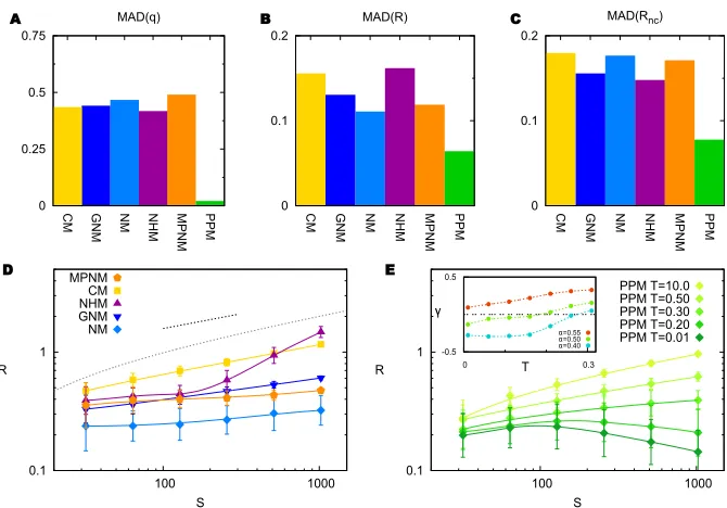
Figure 3. A: Mean Absolute Deviations (MAD) from empirical values of the

incoherence parameter,q, for each food-web model – Cascade (CM),

Generalized Niche (GNM), Niche (NM), Nested Hierarchy (NHM), Minimum Potential Niche (MPNM) and Preferential Preying (PPM) – as compared to a dataset of 46 food webs. B: MAD from empirical values of stability, R, for the same models and food webs as in panelA. C: MAD from empirical values of stability,R, after removing self-links, for the same models and food webs as in panelsAandB.D: Scaling of stability,R, with size,S, in networks generated with each of the models of previous panels except for the PPM. Mean degree is K=√S. The dashed line indicates the slope predicted for random matrices by May [1], while the dotted curve is from Allesina and Tang [27]. E: Scaling of stability,R, with size,S, in PPM networks generated with different values ofT. In descending order,T = 10, 0.5, 0.3, 0.2 and 0.01. B= 0.25S. Inset: Slope, γ, of the stability-size line againstT forα= 0.55, 0.5 and 0.4, where the mean degree isK=Sα_{. In panelsDandE, bars on the symbols are for} one standard deviation.

αlies somewhere between zero and 1/2 [12, 26, 44]. The most recent empirical estimate we are aware of is close to α ≃ 0.5, depending slightly on whether predation weights are considered [45]. In our dataset, the best fit is achieved with a slightly lower exponent, α= 0.41.

In Fig. 3D we show how stability scales with S in each of the niche-based models when complexity increases with size according toα= 0.5. The dashed line shows the slope that May predicted for random networks (R∼√K=S0.25₎

the Nested Hierarchy Model, in which R increases more rapidly at high S), and, as expected, networks always become less stable with increasing size and complexity. In Fig. 3E we show how the stability of PPM networks scales in the same scenario. For highT, their behaviour is similar to that of the Cascade Model: R ∼ Sγ_{, with γ ≃ 0.25. However, the exponent γ decreases as T is} lowered, until, for sufficiently large and coherent networks, it becomes negative – in other words,stability increases with size and complexity. The inset in Fig. 3E shows the exponent γ obtained against T, for different values of α. The smallerα, the larger the range ofT which yields a positive complexity-stability relationship.4

In Section 3.2.1 of Supporting Information we extend this analysis to specific dynamics – Lotka-Volterra, type II and type III – by assuming an exponential relationship between biomass and trophic level which can be described as a pyramid. The positive complexity-stability relationship does not appear to de-pend on the details of dynamics. However, the slope of theR−S curve varies with both the squatness of the biomass pyramid and the extent to which the pyramid is corrupted by noise. A squat pyramid (more biomass at low trophic levels than at high ones) has the strongest relationship, while for an inverted pyramid (more biomass at high trophic levels than at low ones) the slope can flatten out or change sign. Noise in the biomass pyramid tends always to weaken the positive complexity-stability relationship, and can also change its sign.

Discussion

The predation matrices corresponding to real ecosystems are clearly peculiar in some way, since their largest eigenvalues do not depend solely on their size or complexity, as we would expect both from random graph theory and struc-tural food-web models. This is in keeping with the empirical observation that large, complex ecosystems are particularly stable, but challenges current think-ing on food-web architecture. We have shown that the structural property we call trophic coherence is significantly correlated with food-web stability, despite other differences between the ecosystems and the variety of empirical methods used in gathering the data. In fact, cannibalism and trophic coherence together account for most of the variance in stability observed in our dataset. Fur-thermore, we have proved that a maximally coherent food web with constant interaction strengths will always be stable.

We have suggested the Preferential Preying Model as a simple algorithm for generating networks with tunable trophic coherence. Although this model does not attempt to replicate other characteristic features of food webs – such as a phylogenetic signal or body-size effects – it reproduces the empirical stability of the 46 webs analysed quite accurately once its only free parameter has been adjusted to the empirical degree of trophic coherence. Most remarkably, the model predicts that networks should become more stable with increasing size and complexity, as long as they are sufficiently coherent and the number of

4

links does not grow too fast with size. Although this result should be followed up with further analytical and empirical research, it suggests that we need no longer be surprised at the high stability of large, complex ecosystems.

We must caution that these findings do not imply that trophic coherence was somehow selected for by the forces of nature in order to improve food-web function. It seems unlikely that there should be any selective pressure on the individuals making up a species to do what is best for their ecosystem. Rather, many biological features of a species are associated with its trophic level. Therefore, adaptations which allow a given predator to prey on species A are likely to be useful also in preying on species B if A and B have similar trophic levels. This leads to trophic coherence, which results in high stability.

If stability decreased with size and complexity, as previous theoretical studies have assumed, ecosystems could not grow indefinitely, for they would face a cut-off point beyond which they would become unstable [26]. On the other hand, if real ecosystems are coherent enough that they become more stable with size and complexity, as our model predicts, then the reverse might be true. We must also bear in mind, however, that our results are only for linear stability, whereas

structural stability, for instance, may depend differently on size and coherence, and could become the limiting factor [18]. In any case, ascertaining whether the loss of a few species would stabilise or destabilise a given community could be important for conservation efforts, particularly for averting “tipping points” [14].

The findings we report here came about by studying food webs. However, directed networks of many kinds transport energy, matter, information, capital or other entities in a similar way to how food webs carry biomass from producers to apex predators. It seems likely that the relation between a network’s trophic coherence and its leading eigenvalue will be of consequence to other disciplines, and perhaps the Preferential Preying Model, though overly simplistic for many scenarios, may serve as a first approximation for looking into these effects in a variety of systems.

Methods

Measuring stability

Let us assume that the populations of species making up an ecosystem (each characterised by its total biomass) change through time according to some set of nonlinear differential equations, the interactions determined by the predation matrix, A (whose elementsaij take the value one if species i preys on species j, and zero otherwise). If the system persists without suffering large changes it must, one assumes, find itself in the neighbourhood of a fixed point of the dynamics. We can study how the system would react to a small perturbation by expanding the equations of motion around this fixed point and keeping only linear terms. The subsequent effect of the perturbation is then determined by the corresponding Jacobian matrix, and the system will tend to return to the fixed point only if the real parts of all its eigenvalues are negative [22].

not all the biomass lost by a prey species when consumed goes to form part of the predator – in fact, this efficiency is relatively low [48]. It is therefore natural to assume that the effect of species j on species i will be mediated bywij =ηaij−aji, where η is an efficiency parameter which, without further information, we can consider equal for all pairs of species. We can thus treat the interaction matrixW =ηA−AT _{as the Jacobian of some unspecified dynamics.} However, we have ignored the stabilising effect of intra-species competition – the fact that individuals within a species compete with each other in ways which are not specified by the predation matrix. This would correspond to real values to be subtracted from the diagonal elements ofW, thereby shifting its set of eigenvalues (or spectrum) leftwards along the real axis. Therefore, the eigenvalue with largest real part of W, as defined above, can be seen as a measure of the minimum intra-species competition required for the system to be stable. Thus, the lower this value,R=Re(λ1), the higher the stability.

In Section 3.2 of Supporting Information, we describe this analysis in more detail. Beginning with a general consumer-resource differential equation for the biomass of each species, we obtain the Jacobian in terms of the function F(xi, xj) which describes the extent to which speciesiconsumes speciesj. For the simple (and unrealistic) caseF =xi+xj, the Jacobian reduces to the matrix W as given above, independently of the fixed point. For more realistic dynamics, the Jacobian depends on the fixed point. For instance, for the Lotka-Volterra functionF =xixj, the off-diagonal elements of the Jacobian areJij =wijxi. If we setF =xiH(xj) (withH(x) =xh_/(xh_+xh

0),x0 the half-saturation density

and hthe Hill coefficient), we have either type II (h= 1) or type III (h= 2) dynamics [49]. Then the off-diagonal elements areJij= [˜η(xi, xj)aij−aji]H(xi), where the effective efficiency is ˜η(xi, xj) =ηhxh

0xix

−(h+1)

j H(xj)2/H(xi). The Jacobians for Lotka-Volterra, type II and type III dynamics are all similar in form to the matrix W, although for an exact solution we require the fixed point. In the main text we therefore use the leading eigenvalue of W as a generic measure of stability. However, in Section 3.2.1 of Supporting Information we consider the effects that different kinds of biomass distribution have on each of these more realistic dynamics. The results are qualitatively the same as those for the matrixW, although we find that both the squatness of a biomass pyramid and the level of noise in this structure affect the strength of the diversity-stability relationship described in the main text.

This measure of stability depends on the parameterη. In Section 3.2.2 of Supporting Information we show that the results reported here remain qualita-tively unchanged for any η ∈(0,1), and discuss how stability is affected when we consider η >1 or η <0. We also look into the effects of including a noise term so that η does not have the same value for each pair of species, and find that our results are robust to this change too. For the results in the main text, however, we use the fixed valueη= 0.2.

Trophic levels and coherence

The trophic levelsiof speciesiis defined as the average trophic level of its prey, plus one [19]. That is,

si= 1 + 1 kin

i X

j

wherekin i =

P

jaij is the number of prey of speciesi(ori’sin-degree), andaij are elements of the predation matrixA. Basal species (those with kin_{= 0) are} assigneds= 1. The trophic level of each species is therefore a purely structural (i.e. topological) property which can be determined by solving a system of linear equations. Since we only consider unweighted networks here (the elements ofA are ones and zeros), we omit the link strength term usually included in Eq. (1) [19].

We can write Eq. (1) in terms of a modified graph Laplacian matrix, Λs=v, where s is the vector of trophic levels, v is the vector with elements vi = max(kin

i ,1), and Λ = diag(v)−A. Thus, every species can be assigned a trophic level if and only if Λ is invertible. This requires at least one basal species (else zero would be an eigenvalue of Λ). However, note that cycles are not, in general, a problem, despite the apparent recursivity of Eq. (1)

We define the “trophic distance” spanned by each link (aij = 1) as xij = si −sj (which is not a distance in the mathematical sense since it can take negative values). The distribution of trophic distances over the network isp(x), which will have meanhxi= 1 (since for any nodeithe average over its incoming links isP

jaij(si−sj)/k in

i = 1 by definition). We define the “trophic coherence” of the network as the homogeneity ofp(x): the more similar the trophic distances of all the links, the more coherent. As a measure of coherence, we therefore use the standard deviation of the distribution, which we refer to as an incoherence parameter: q=phx2_{i −1, whereh·i=L}−1P

ij(·)aij, andLis the total number of links,L=P

ijaij.

Trophic coherence bears a close resemblance to Levine’s measures of “trophic specialization” [19]. However, our average is computed over links instead of species, with the consequence that we need not consider the distinction be-tween resource and consumer specializations. It is also related to measures of omnivory: in general, the more omnivores one finds in a community, the less coherent the food web.

The Preferential Preying Model

We begin withBnodes (basal species) and no links. We then add, sequentially, S−B new nodes (consumer species) to the system according to the following rule. A new node i is first awarded a random node j from among all those available when it arrives. Then anotherκi nodeslare chosen with a probability Pil that decays with the trophic distance betweenj and l. Specifically, we use the exponential form

Pil∝exp

−|sj−sl|

T

,

wherej is the first node chosen byi, andT is a parameter that sets the degree of trophic specialization of consumers.

The number of extra prey,κi, is obtained in a similar manner to the Niche Model prescription, since this has been shown to provide the best approximation to the in-degree distributions of food webs [38]. We set κi =xini, whereni is the number of nodes already in the network wheniarrives, andxi is a random variable drawn from a Beta distribution with parameters

β= S

2_−B2

whereLis the expected number of links. In this work, we only consider networks with a number of links within an error margin of 5% of the desiredL; thus, for all the results reported, we have imposed this filter on the PPM networks and those generated with the other models.

To allow for cannibalism, the new node i is initially considered to have a trophic levelsi=sj+ 1 according to which it might then choose itself as prey. Onceihas been assigned all its prey, si is updated to its correct value.

Acknowledgements

References

[1] R. M. May, “Will a large complex system be stable,” Nature, vol. 238, pp. 413–14, 1972.

[2] R. M. May,Stability and complexity in model ecosystems. Princeton, USA: Princeton University Press, 1973.

[3] R. MacArthur, “Fluctuations of animal populations, and a measure of community stability,” Ecology, vol. 36, pp. 533–5, 1955.

[4] R. Paine, “Food web complexity and species diversity,”Am. Nat., vol. 100, pp. 65–75, 1966.

[5] K. S. McCann, “The diversity-stability debate,”Nature, vol. 405, pp. 228– 33, 2000.

[6] J. A. Dunne, U. Brose, R. J. Williams, and N. D. Martinez, “Model-ing food-web dynamics: complexity-stability implications,” Aquatic Food Webs: An Ecosystem Approach, pp. 117–129, 2005.

[7] C. S. Elton,Ecology of Invasions by Animals and Plants. London: Chap-man and Hall, 1958.

[8] D. L. DeAngelis and J. C. Waterhouse, “Equilibrium and nonequilibrium concepts in ecological models,” Ecol. Monogr., vol. 57, pp. 1–21, 1987.

[9] U. Brose, R. J. Williams, and N. D. Martinez, “Allometric scal-ing enhances stability in complex food webs,” Ecology Letters, vol. 9, p. 1228–1236, 2006.

[10] C. Jacquet, C. Moritz, L. Morissette, P. Legagneux, F. Massol, P. Ar-chambault, and D. Gravel, “No complexity-stability relationship in natu-ral communities,”arXiv:1307.5364, 2013.

[11] C. S. Elton,Animal Ecology. London: Sidgwick and Jackson, 1927.

[12] S. L. Pimm,The Balance of Nature? Ecological Issues in the Conservation of Species and Communities. Chicago: The University of Chicago Press, 1991.

[13] R. V. Sol´e and J. Bascompte,Self-Organization in Complex Ecosystems. Princeton, USA: Princeton University Press, 2006.

[14] W. J. Sutherland, R. P. Freckleton, H. C. J. Godfray, S. R. Beissinger, T. Benton, D. D. Cameron, Y. Carmel, D. A. Coomes, T. Coulson, M. C. Emmerson, R. S. Hails, and G. C. Hays, “Identification of 100 fundamental ecological questions,” Journal of Ecology, vol. 101, pp. 58–67, 2013.

[15] S. L. Pimm,Food Webs. London: Chapman and Hall, 1982.

[17] B. Drossel and A. J. McKane,“Modelling Food Webs”, in A Handbook of Graphs and Networks: From the Genome to the Internet. Berlin: Wiley-VCH, 2003.

[18] A. G. Rossberg,Food Webs and Biodiversity: Foundations, Models, Data. Wiley, 2013.

[19] S. Levine, “Several measures of trophic structure applicable to complex food webs,”J. Theor. Biol., vol. 83, pp. 195–207, 1980.

[20] D. Pauly, V. Christensen, J. Dalsgaard, R. Froese, and F. Torres, “Fishing down marine food webs,”Science, vol. 279, pp. 860–3, 1998.

[21] V. Grimm and C. Wissel, “Babel, or the ecological stability discussions: An inventory and analysis of terminology and a guide for avoiding confu-sion,”Oecologia, vol. 109, pp. 323–334, 1997.

[22] P. Holmes and E. T. Shea-Brown, “Stability,”Scholarpedia, vol. 1, p. 1838, 2006.

[23] R. M. May, “Qualitative stability in model ecosystems,”Ecology, vol. 54, pp. 638–41, 1973.

[24] D. O. Logofet, “Stronger-than-Lyapunov notions of matrix stability, or how “flowers” help solve problems in mathematical ecology,” Linear Al-gebra and its Applications, vol. 398, pp. 75–100, 2005.

[25] D. O. Logofet,Matrices and Graphs: Stability Problems in Mathematical Ecology. Boca Raton: CRC Press, 1993.

[26] R. Sol´e, D. Alonso, and A. McKane, “Scaling in a network model of a multispecies ecosystem,”Physica A, vol. 286, pp. 337–44, 2000.

[27] S. Allesina and S. Tang, “Stability criteria for complex ecosystems,” Na-ture, vol. 483, pp. 205–8, 2012.

[28] G. Caldarelli, P. G. Higgs, and A. J. McKane, “Modelling coevolution in multispecies communities,”J. Theor. Biol., vol. 193, pp. 345–58, 1998.

[29] U. Bastolla, M. Laessig, S. Manrubia, and A. Valleriani, “Diversity pat-terns from ecological models at dynamical equilibrium,” J. Theor. Biol., vol. 212, pp. 11–34, 2001.

[30] N. Loeuille and M. Loreau, “Evolutionary emergence of size-structured food webs,”Proc. Natl. Acad. Sci. USA, vol. 102, p. 5761, 2005.

[31] A. G. Rossberg, H. Matsuda, T. Amemiya, and K. Itoh, “Food webs: experts consuming families of experts,”J. Theor. Biol., vol. 241, pp. 552– 63, 2006.

[32] A. J. McKane and B. Drossel,Models of food web evolution, in Ecological Networks: Linking Structure to Dynamics in Food Webs. M. Pascual and J.A. Dunne, eds. Oxford, UK: Oxford University Press, 2006.

[34] A. G. Rossberg, A. Br¨annstr¨om, and U. Dieckmann, “Food-web structure in low- and high-dimensional trophic niche spaces,”Journal of The Royal Society Interface, 2010.

[35] R. J. Williams and N. D. Martinez, “Simple rules yield complex food webs,”Nature, vol. 404, pp. 180–183, 2000.

[36] R. J. Williams and N. D. Martinez, “Success and its limits among struc-tural models of complex food webs,” Journal of Animal Ecology, vol. 77, pp. 512–519, 2008.

[37] J. E. Cohen and C. M. Newman, “A stochastic theory of community food webs I. models and aggregated data,”Proc. R. Soc. London Ser. B., vol. 224, pp. 421–448, 1985.

[38] D. B. Stouffer, J. Camacho, R. Guimer`a, C. A. Ng, and L. A. N. Amaral, “Quantitative patterns in the structure of model and empirical food webs,”

Ecology, vol. 86, p. 1301–1311, 2005.

[39] D. B. Stouffer, J. Camacho, and L. A. N. Amaral, “A robust measure of food web intervality,” Proc. Natl. Acad. Sci. USA, vol. 103, pp. 19015– 19020, 2006.

[40] S. Allesina, D. Alonso, and M. Pascual, “A general model for food web structure,”Science, vol. 320, pp. 658–661, 2008.

[41] M. F. Cattin, L. F. Bersier, C. Banasek-Richter, R. Baltensperger, and J. P. Gabriel, “Phylogenetic constraints and adaptation explain food-web structure,”Nature, vol. 427, pp. 835–9, 2004.

[42] A. L. Barab´asi and R. Albert, “Emergence of scaling in random networks,”

Science, vol. 286, pp. 509–512, 1999.

[43] R. Thompson and C. Townsend, “Impacts on stream food webs of na-tive and exotic forest: an intercontinental comparison,” Ecology, vol. 84, pp. 145–61, 2003.

[44] A. G. Rossberg, K. D. Farnsworth, K. Satoh, and J. K. Pinnegar, “Univer-sal power-law diet partitioning by marine fish and squid with surprising stability-diversity implications,” Proc. R. Soc. B, vol. 278, pp. 1617–25, 2011.

[45] C. Banaˇsek-Richter, L. Bersier, M. Cattin, R. Baltensperger, J. Gabriel, and J. Merz, et al., “Complexity in quantitative food webs,” Ecology, vol. 90, pp. 1470–7, 2009.

[46] T. Gross, L. Rudolf, S. Levin, and U. Dieckmann, “Generalized models reveal stabilizing factors in food webs,” Science, vol. 325, pp. 747–50, 2009.

[48] R. L. Lindeman, “The trophic-dynamic aspect of ecology,” Ecology, vol. 23, pp. 399–418, 1942.

arXiv:1404.7728v3 [q-bio.PE] 24 Nov 2014

Trophic coherence determines food-web stability

Supporting Information

Samuel Johnson,

Virginia Dom´ınguez-Garc´ıa,

Luca Donetti,

and

Miguel A. Mu˜

noz

1

Warwick Mathematics Institute, and Centre for Complexity Science,

University of Warwick, Coventry CV4 7AL, United Kingdom. 3

Departamento de Electromagnetismo y F´ısica de la Materia, and

Instituto Carlos I de F´ısica Te´orica y Computacional,

Universidad de Granada, 18071 Granada, Spain. 4

Departamento de Electr´onica y Tecnolog´ıa de Computadores, and Centro de Investigaci´on en Tecnolog´ıas de la Informaci´on y de las Comunicaciones,

Universidad de Granada, 18071 Granada, Spain.

Contents

1 Food-web models 3

1.1 The Cascade Model . . . 3

1.2 The Niche Model . . . 3

1.3 The Nested Hierarchy Model . . . 4

1.4 The Generalized Niche Model . . . 4

1.5 The Minimum Potential Niche Model . . . 5

1.6 The Preferential Preying Model . . . 5

1.6.1 Possible amendments to the PPM . . . 5

1.6.2 Negative temperatures . . . 7

2 Food-web data 8 3 Network measures 10 3.1 Trophic coherence . . . 10

3.2 Stability . . . 10

3.2.1 Biomass distribution . . . 13

3.2.2 Efficiency . . . 17

3.2.3 Herbivory . . . 20

3.2.4 Weighted networks . . . 20

3.2.5 Feasibility . . . 22

3.2.6 Stability criteria . . . 22

3.2.7 Missing links and trophic species . . . 23

3.3 Mean chain length . . . 24

3.4 Modularity . . . 25

3.5 Cannibals and apex predators . . . 26

3.6 Mean trophic level . . . 26

3.7 Comparison of network measures . . . 27

4 Analytical theory for maximally coherent

networks 31

1

Food-web models

We describe here the main structural (also called static) models found in the literature for generating networks with some of the statistical features of food webs. We then discuss some aspects of the Preferential Preying Model (PPM) which we put forward in the main text (described in Methods). In all these models, the number of links L can only be set in expected value. As is often done, throughout this work we discard all generated networks which have a number of links greater or smaller than this targetLby more than five percent. In Section 3 we describe several network measures and compare the performance of the models using the food-web data listed in Section 2.

1.1

The Cascade Model

In the Cascade Model, each species i is assigned a random number ni drawn from a uniform distribution between 0 and 1 [1]. For any pair (i,j), we setito be a consumer ofjwith a constant probabilitypifni> nj, and with probability zero ifni≤nj. WithS species, we obtain an expected number of linksLif we set

p= 2L S(S−1).

This was the first attempt to show how networks with a structure in some senses similar to real food webs could come about via simple rules.

Stouffer and co-workers later modified this model so that the number of prey would be drawn from the Beta distribution used by the Niche Model (see below), and called the new version the Generalized Cascade Model [2]. Since this amendment improves the model’s predictions as regards distributions of prey and predators (without, to the best of our knowledge, involving any drawbacks), throughout this paper we use the Generalized Cascade Model.

1.2

The Niche Model

In the Niche Model, each species i is awarded a niche value ni as in the Cas-cade Model [3]. However, instead of choosing species with lower niche values randomly for prey,iis constrained to consume the subset of speciesjsuch that ci−ri/2 ≤ nj < ci+ri/2 – i.e., all those lying on an interval of the niche axis of size ri and centred at ci, and none without. The range is defined as ri =xini, wherexi is drawn from a Beta distribution with parameters (1, β). ForS species and a desired number of linksL, we must set

β= S(S−1) 2L −1.

The centre of the intervalciis drawn from a uniform distribution betweenri/2 andmin(ni,1−ri/2).

The rationale behind this model was that food webs were thought to be

outperforms the Cascade Model in approximating measurable features of food webs, and even compares well to more elaborate models which take the Niche Model as a basis [7]. It is still the model most commonly used whenever synthetic networks similar to food webs are required.

1.3

The Nested Hierarchy Model

The Nested Hierarchy Model provides a way to take into account that phyloge-netically similar species should have prey in common [8]. It gives each species a niche value and a range, exactly as in the Niche Model. However, instead of establishing links directly to species within the range, first the number of prey to be consumed by each species is determined, in proportion to the range, kin

i ∝ ri, so as to generate an expected number of links L. These links are then attributed in the following way. The species with lowest niche value has no prey, while the one with the highest has no predators (so there is always at least one basal species and one apex predator). Starting from the species with second smallest niche value and going up in order ofn, we take each species i and apply the following rules to determine itskin

i prey:

1. We choose a random speciesj already in the network (sonj ≤ni) and set it as the first prey species ofi.

2. Ifj has no predators other thani, we repeat 1 until either the chosen prey does have other predators, or we reachkin

i . Else we go to 3.

3. We determine the set of species which are prey to the predators of j. We select, randomly, species from this set to become also prey of iuntil we either completekin

i , or we go to 4.

4. We continue choosing prey species randomly from among those with lower niche values. If we still have not reachedkin

i when these run out, we continue choosing them randomly from those with higher niche values.

In this model, two consumers that share prey are assumed to be phyloge-netically related, while the extra links that must at times be sought mimic the effects of independent adaptation. We find it a particularly interesting model because phylogenetic constraints should indeed be taken into account, and as it stands our Preferential Preying Model (described below) does not do this. One problem we find with the Nested Hierarchy Model, however, is that a given species i is assumed to be related to a certain set A of species which share common prey with i; but i will also belong to the set B of common prey of a different set of consumers, and nothing constrainsAandBto overlap. In other words, the species related toidue to its prey are not the ones related toidue to its predators, whereas in nature it is to be expected that phylogenetically similar species should have both prey and predators in common. In fact, it has recently been reported that common predators are statistically more significant than common prey [9].

1.4

The Generalized Niche Model

Model would be implemented as before but with reduced ranges ri = cxini. Then, for each species, the number of extra prey kcascade

i = (1−c)xiniS is drawn randomly from among the available species with niche values lower than ni, as in the Generalized Cascade Model. Forc= 1 we have the Niche Model, whilec= 0 results in the Generalized Cascade Model.

The Generalized Niche Model has been shown to emulate real food webs very successfully, at least as regards certain features, such as community structure [10]. It is also often used as a convenient model for generating synthetic networks with a view to studying food websin silico [11].

1.5

The Minimum Potential Niche Model

The Minimum Potential Niche Model is similar to the Generalized Niche Model in that it is a modification of the Niche Model which breaks up complete in-tervality by means of a parameter, f [12]. However, the motivation is slightly different. The idea is that in reality there is more than one niche dimension con-straining possible predation links (hence the lack of complete, one-dimensional intervality), which implies that some of the links determined by the Niche Model are actually “forbidden links”. The species are all allocated niche valuesni and ranges ri = xini as in the Niche Model. The species at the extremes of this range are always consumed. However, the rest is considered a potential range and the β parameter used in the Beta distribution from which xi is drawn is now

β= S(S−1) 2(L+F)−1,

where F = f P, P being the total number of potential links given the ranges, minus the species at the extremes. Once all the species have their ranges, each species within will be consumed with a probability 1−f. Therefore,f = 0 results in the original Niche Model, butf >0 produces a proportion of forbidden links. Allesinaet al. suggested a framework for comparing niche-based models [12]; they computed the likelihood that the Cascade, Niche and Nested Hierarchy models have of generating the links in a set of ten real food webs, and found theirs (the Minimum Potential Niche Model) to be superior – and, in fact, the only one capable of generating all the observed links.

1.6

The Preferential Preying Model

In the main text we propose the Preferential Preying Model (PPM) in order to capture the trophic coherenceof empirical food webs. The details are given in Methods, so here we confine ourselves to displaying the scheme diagrammatically in Fig. S1. We go on to list several possible amendments which could be made to this basic version of the model and which may be of use to researchers wishing to use the PPM for purposes other than our main one here – namely, to highlight the importance of trophic coherence and its relevance to food-web stability.

1.6.1 Possible amendments to the PPM

Figure S 1. Diagram showing how networks are assembled in the Preferential Preying Model (PPM), as described in Methods in the main text. In PanelA a new node, labelledi, is introduced to the networks, and is randomly assigned node 4 as its first prey species. In PanelB, the probabilities of next choosing node 5 or node 6 are calculated, as functions of their trophic distance to node 4 (β = 1/T). Node 5 is the closest, and in this case is taken as the second prey species, as shown in PanelC.

set number of basal species, as in the Preferential Attachment Model [13]. We imagine that for most applications where synthetic networks are re-quired it would be useful to have control over this parameter (which is itself related to trophic coherence, as we show in Section 3.2.3). However, if a freely emerging B were preferred – for instance, for a rigorous com-parison against models which do not allow this value to be set easily – it is straightforward to take the minimum κi equal to zero for incoming species, thereby allowing a proportion of them to become producers.

• Numbers of prey. We have drawn the number of prey for each incoming species from a Beta distribution, as in all the niche-based models, because Stoufferet al. [2] have shown that this method yields a particularly good fit to food-web data (we have also verified that this holds true for our 46 food-web dataset). However, were the model to be applied to systems other than food webs, it may be preferable to use, for instance, a Poisson or a Pareto distribution, depending on the in-degree distributions of the networks to be emulated.

• Boltzmann factor. The functional form we have used to determine the second and subsequent prey of an incoming species (an exponential in the trophic distance divided by the parameterT) is arbitrary; careful fitting to data may suggest a better function. There is also no reason other than simplicity to use the same value ofT for each incoming species: one could also draw a different valueTi for each incoming species form some distribution, perhaps dependent on the trophic level of its first prey.

• Phylogeny and body size. In this simple incarnation, the PPM ignores the main effects that most of the other models are based on, but these could be taken into account in a “Generalized Preferential Preying Model”. Something akin to a phylogenetic signal could be induced by introducing a bias in the Boltzmann factor such that an incoming node tended to copy the prey and predators of a randomly chosen species already in the network – perhaps limiting in the Nested Hierarchy Model in the case where only prey are copied. The Niche, Generalized Niche and Minimum Potential Niche models assume that the niche ordering (usually thought to represent body size, possibly in combination with other biological features) to some extent constrains species to find prey within closed intervals thereof. A bias could likewise be introduced in the Boltzmann factor of the PPM such that intervals of the sequence of entry were preferred, if this constraint in empirical networks turned out to be more than a spurious effect of trophic coherence.

1.6.2 Negative temperatures

As discussed in the main text, the PPM can generate any level of trophic coher-ence between that of a maximally coherent structure (withT →0) and one as incoherent as would be obtained if attachment were random (atT → ∞). How-ever, as shown in Table S1, some food webs (five out of the 46 in our dataset) exhibit higher values ofqeven than this latter case. The PPM can also generate greater incoherence than obtained at high positiveTwith negative values of this parameter, as illustrated in Fig. S2. The curves ofqandRwould be continuous if instead of T we used its inverse, β = 1/T. With this parameter,β = 0 cor-responds to random attachment, with q falling monotonically from maximum incoherence atβ → −∞to maximum coherence atβ →+∞. A comparison of the two panels in Fig. S2 shows that the effect of trophic coherence on stability seems to saturate at about the q obtained with random attachment: greater incoherence has little effect onR.

0 0.2 0.4 0.6 0.8 1

-2 -1 0 1 2

q T 0 0.2 0.4 0.6 0.8 1

-2 -1 0 1 2

q T 0 0.2 0.4 0.6 0.8 1

-2 -1 0 1 2

q T 0 0.1 0.2 0.3 0.4 0.5

-2 -1 0 1 2

R T 0 0.1 0.2 0.3 0.4 0.5

-2 -1 0 1 2

R T 0 0.1 0.2 0.3 0.4 0.5

-2 -1 0 1 2

R

T

2

Food-web data

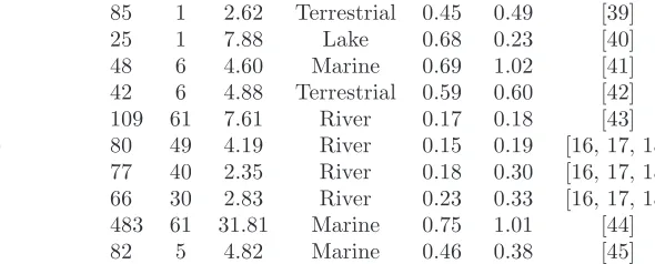
We have compiled a dataset of 46 food webs available in the literature, pertaining to several ecosystem types. The methods used by the researchers to establish the links between species vary from gut content analysis to inferences about the behaviour of similar creatures. In Table S1 we list the food webs used along with references to the relevant work. We also list, for each case, the number of species S, of basal species B, the mean degree K, the ecosystem type, the trophic coherenceq, the value of the parameter T found to yield (on average) the empirical q with the Preferential Preying Model, and the numerical label used to represent the food web in several figures below.

Food web S B K Type q T Reference Label

Akatore Stream 84 43 2.70 River 0.16 0.26 [16, 17, 18] 18

Benguela Current 29 2 7.00 Marine 0.76 0.87 [19] 11

Berwick Stream 77 35 3.12 River 0.18 0.25 [16, 17, 18] 34

Blackrock Stream 86 49 4.36 River 0.19 0.25 [16, 17, 18] 27

Bridge Brook Lake 25 8 4.28 Lake 0.59 1.15 [20] 14

Broad Stream 94 53 6.01 River 0.16 0.16 [16, 17, 18] 35

Canton Creek 102 54 6.83 River 0.16 0.18 [21] 2

Caribbean (2005) 249 5 13.31 Marine 0.75 0.70 [22] 17

Caribbean Reef 50 3 11.12 Marine 0.99 -0.24 [23] 13

Carpinteria Salt Marsh Reserve 126 50 4.29 Marine 0.65 -8.27 [24] 33

Catlins Stream 48 14 2.29 River 0.20 0.27 [16, 17, 18] 19

Chesapeake Bay 31 5 2.19 Marine 0.47 0.67 [14, 15] 5

Coachella Valley 29 3 9.03 Terrestrial 1.34 -0.02 [25] 12

Crystal Lake (Delta) 19 3 1.74 Lake 0.28 0.33 [26] 37

Cypress (Wet Season) 64 12 6.86 Terrestrial 0.63 0.73 [27] 42

Dempsters Stream (Autumn) 83 46 5.00 River 0.23 0.30 [16, 17, 18] 36

El Verde Rainforest 155 28 9.74 Terrestrial 1.02 -0.82 [28] 15

Everglades Graminoid Marshes 63 5 9.79 Terrestrial 0.66 0.47 [29] 44

Florida Bay 121 14 14.60 Marine 0.59 0.48 [27] 26

German Stream 84 48 4.20 River 0.21 0.29 [16, 17, 18] 28

Grassland (U.K) 61 8 1.59 River 0.40 0.72 [30] 4

Healy Stream 96 47 6.60 River 0.22 0.24 [16, 17, 18] 29

Kyeburn Stream 98 58 6.42 River 0.18 0.18 [16, 17, 18] 30

LilKyeburn Stream 78 42 4.81 River 0.23 0.29 [16, 17, 18] 31

Little Rock Lake 92 12 10.84 Lake 0.69 0.75 [31] 8

Lough Hyne 349 49 14.66 Lake 0.62 0.66 [32, 33] 46

Mangrove Estuary (Wet Season) 90 6 12.79 Marine 0.67 0.47 [27] 43

Martins Stream 105 48 3.27 River 0.32 0.49 [16, 17, 18] 20

Maspalomas pond 18 8 1.33 Lake 0.48 -9.22 [34] 39

Michigan Lake 33 5 3.91 Lake 0.38 0.21 [35] 40

Mondego Estuary 42 12 6.64 Marine 0.74 10.07 [36] 41

Narragansett Bay 31 5 3.65 Marine 0.66 1.18 [37] 38

Narrowdale Stream 71 28 2.18 River 0.25 0.38 [16, 17, 18] 21

N.E. Shelf 79 2 17.76 Marine 0.82 0.67 [38] 10

North Col Stream 78 25 3.09 River 0.28 0.34 [16, 17, 18] 22

Scotch Broom 85 1 2.62 Terrestrial 0.45 0.49 [39] 16

Skipwith Pond 25 1 7.88 Lake 0.68 0.23 [40] 6

St. Marks Estuary 48 6 4.60 Marine 0.69 1.02 [41] 9

St. Martin Island 42 6 4.88 Terrestrial 0.59 0.60 [42] 7

Stony Stream 109 61 7.61 River 0.17 0.18 [43] 3

Sutton Stream (Autum) 80 49 4.19 River 0.15 0.19 [16, 17, 18] 32

Troy Stream 77 40 2.35 River 0.18 0.30 [16, 17, 18] 24

Venlaw Stream 66 30 2.83 River 0.23 0.33 [16, 17, 18] 25

Weddell Sea 483 61 31.81 Marine 0.75 1.01 [44] 45

Ythan Estuary 82 5 4.82 Marine 0.46 0.38 [45] 1

3

Network measures

3.1

Trophic coherence

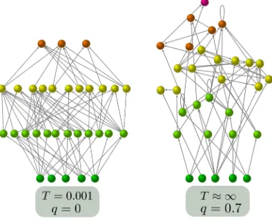
In the Methods section of the main text we define the network structural prop-erty of trophic coherence. Here we simply illustrate the difference between a maximally coherent network and a highly incoherent one in Fig. S3.

Figure S 3. Two example networks generated with the Preferential Preying Model, illustrating the extremes of trophic coherence: the network on the left was generated withT = 0.001 and hasq= 0 (all links are between species exactly one trophic level apart) while the one on the right is forT = 10 (almost random attachment) and hasq= 0.7.

In Fig. S4 we show the empirical values of q observed in each of the 46 food webs (also displayed in Table S1) along with the predictions of each of the food-web models discussed above and in the main text.

3.2

Stability

Let us assume that we have a set of ordinary differential equations governing the evolution of the population of each species in an ecosystem, as measured, for instance, by its total biomassxi. In vector form, we can write this as

d

dtx=f(x).

The dynamics will have a fixed point at any configurationx∗_{such thatf(x}∗_{) =}

0. Let us suppose that the system is placed at this fixed point but suffers a small perturbationζζζ(t):

x(t) =x∗

+ζζζ(t).

For small enough|ζζζ(t)|, its dynamics will be given by the linearised equation:

d

dtζζζ(t) =J(x

∗

0 0.2 0.4 0.6 0.8 1 1.2 1.4 1.6 1.8

2 4 6 8 10 12 14 16 18

q

0 0.2 0.4 0.6 0.8 1 1.2 1.4

20 22 24 26 28 30 32 34 36

q

0 0.2 0.4 0.6 0.8 1 1.2 1.4 1.6

38 40 42 44 46 48 50 52 54

q

CM ONM NHM GNM MPNM PPM real

Figure S 4. Trophic coherence, as measured byq, for each of the food webs listed in Table S1. The corresponding predictions of each food-web model discussed in Section S1 – Cascade, Niche, Nested Hierarchy, Generalized Niche, Minimum Potential Niche and Preferential Preying – are displayed with bars representing one standard deviation about the mean. Empirical values are black squares. The labelling of the food webs is indicated in the rightmost column of Table S1.

where J(xxx∗_{) is the Jacobian matrix [∂fi/∂xj] evaluated atxxx}∗_{. The fixed point}

will be locally stable if all the eigenvalues ofJ(xxx∗_{) have negative real part [46].}

Let us consider a fairly general dynamics forxxx∗_{given by a consumer-resource}

model:

d

dtxi =ηij

X

j

aijF(xi, xj)−X j

ajiF(xj, xi) +G(xi). (1)

parameter toη= 0.2.

The Jacobian,J, will be obtained by taking the partial derivatives of Eq. (1), for eachi, with respect to eachxj.

In the simple case where the interaction between species is given by a sum,

F(xi, xj) =xi+xj,

we have

Jij = (ηaij−aji)(1 +δij) +γδij,

whereδij is the Kronecker delta (equal to one wheni=j, or else zero). Positive terms added to or subtracted from the main diagonal ofJ simply shift its spec-trum of eigenvalues to the right or left, respectively. Therefore, we concentrate on the matrix

W =ηA−AT, (2)

where AT _{is the transpose of A, and consider λ}

1, the eigenvalue of W with

the largest real part. Then, R = Re(λ1) can be regarded as a measure of

the minimum degree of self-regulation at each node which this dynamics would require in order for the system to be stable. In other words, the smallerR, the more stable we shall say the system is.

In this simple case defined byF(xi, xj) =xi+xj the Jacobian is indepen-dent of the pointxxx∗

where it is evaluated. However, this will not, in general, be the case and for other dynamics we would need to specify this point in or-der to characterise the stability of the system. For instance, in a generalised Lotka-Volterra dynamics, the interaction is proportional to the biomass of both consumer and resource,

F(xi, xj) =xixj,

and the Jacobian becomes

Jij = (1 +δij)wijxi+γδij, (3)

wherewij are the elements of the matrixW as given by Eq. (2). Note that this expression depends on the biomass of speciesi(though not onj’s) at the point of interest.

To capture the nonlinearities expected in a prey species’ functional response, consumer-resource models often describe the interaction as

F(xi, xj) =xiH(xj),

whereH is the Hill equation,

H(x) = x h

xh

0+xh

,

with x0 the half-saturation density. The Hill coefficient hdetermines whether

the functional response is of type II (h= 1) or type III (h= 2) [47]. Now we find that the Jacobian is

Jij = [˜η(xi, xj)aij−aji]H(xi) (4)

ifi6=j, where the effective efficiency of predation is

˜

η(xi, xj) = xi H(xi)

∂H(xj) ∂xj η =

hxh

0xi

xh_j+1

H(xj)2

and, for the main diagonal elements,

Jii={h[1−H(xi)] + 1}H(xi)wii+γ.

In each of these kinds of dynamics it is necessary to evaluate the Jacobian at a particular point: Equations (3) (Lotka-Volterra) and (4) (types II and III) are similar in form to the matrix W of Eq. (2), but their terms are modified by the biomass of the predator, or the biomasses of both prey and predator, respectively. One might suggest that we only need identify a fixed point and evaluate the equations there. But, in general, a feasible fixed point (in which xi > 0 for all i) will not exist. Feasible fixed points could be defined by at-tributing weights to the elements of the interaction matrix A, but this would involve decisions on how to do this in a realistic way which might render the results somewhat arbitrary. (For a discussion on the feasibility of fixed points, see Section S3.2.5.)

Throughout most of the paper we focus simply on the matrixW as given by Eq. (2), for although the dynamics it describes exactly is not very realistic (corresponding to the interaction termF(xi, xj) =xi+xjin Eq. (1)), it captures the essential behaviour of better motivated dynamics without requiring any assumptions about the fixed point. In fact, if all species had the same biomass at the fixed-point, then Eqs. (3) (Lotka-Volterra) and (4) (types II and III) would also reduce to the matrix W as given by Eq. (2), for an appropriate choice of the parameterη. However, so as to test the robustness of our results to details of the dynamics, in Section S3.2.1 we look into the effects of different distributions of biomass according together with Lotka-Volterra, type II or type III dynamics. We find that the relationship between trophic coherence and stability reported in the main text is robust to these considerations, although the dependence of biomass on trophic level introduces interesting effects, in particular for the complexity-stability scaling.

In the main text we describe how stability in directed networks (and food webs in particular) is determined to a large extent by their trophic coherence. In Fig. S5 we compare the predictions of each of the food-web models described in Section 1 for each of the food webs listed in Table 1. Another network feature which influences stability, as mentioned above, is the existence of self-links (representing cannibalism, in the case of food webs), since this is a form of self-regulation. We disentangle this effect from that of trophic coherence, we remove all self-links from the food webs and again measure the real part of the leading eigenvalue,Rnc. The predictions of each model are shown in Fig. S6.

In Section 4 we give a proof that a maximally coherent network (q= 0) with constant interaction strengths can always be stabilised with an infinitesimal degree of self-regulation.

3.2.1 Biomass distribution