Measuring and modelling patterns of behaviour in datasets of individual investor trading records using flexible methods

(1)

warwick.ac.uk/lib-publications

A Thesis Submitted for the Degree of PhD at the University of Warwick

Permanent WRAP URL:

http://wrap.warwick.ac.uk/101984

Copyright and reuse:

This thesis is made available online and is protected by original copyright. Please scroll down to view the document itself.

Please refer to the repository record for this item for information to help you to cite it. Our policy information is available from the repository home page.

(2)

Measuring and Modelling

Patterns of Behaviour in Datasets

of Individual Investor Trading

Records Using Flexible Methods

by

Matthew Burgess

A thesis submitted to the University of Warwick for the degree of

Doctor of Philosophy

Department of Statistics

(3)

List of Figures

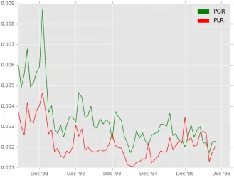
1.1 A monthly time series of the aggregate disposition effect, across all investors and stocks. The component parts are split according to the month they occurred in, and a disposition effect score calculated according to the formula described in Section 1.4. The data run from January 1991 to November 1996. The first few months are very volatile due to a low number of stocks being under observation, hence the figure is started in April 1991. . . 16 1.2 A monthly time series of the proportion of gains realized

(PGR) and the proportion of losses realized (PLR). Or al-ternatively, the proportion of opportunities to sell for a gain or loss that investors take in aggregate. Again the plot is started in April 1991 due to the low amount of data available to calculate the ratios with at the start of the period. . . 18 1.3 The number of sales for a gain and the number of sales for a

loss each month during the data period, across all investors and stocks. . . 19 1.4 The number of days each month, summed across all investors

(7)

1.5 Monthly time series of the disposition effect for stocks in the top 20% of the cap-size distribution (updated annually) and separately for all other stocks. . . 24 1.6 The number of sales for a gain and a loss each month across

all stocks in the bottom 80% of the cap-size distribution. . . 25 1.7 The number of gain and loss days each month for stocks in

the bottom 80% of the cap-size distribution. . . 26 1.8 Plots of the bottom (left) and top (right) 10% of DE influence

scores across all stocks. . . 29 1.9 A plot of a smoothed curve fitted to the scaled Schoenfeld

residuals for the paper gain indicator, with a dashed line at the level of the coefficient estimate β. . . 45

2.1 Plot of a smooth of the scaled Schoenfeld residuals for the interaction term between the paper gain indicator and the ’Limited’ group for self-assessed experience, in the frailty and marginal models. Each curve is plotted with an approximate 95% confidence interval. A horizontal dashed line is plotted at the coefficient estimate for the variable in the respective model. . . 67 2.2 Plot of a smooth of the scaled Schoenfeld residuals for the

(8)

2.3 Plot of a smooth of the scaled Schoenfeld residuals for the interaction term between the paper gain indicator and the gender indicator (equalling one if the investor is male) in the frailty model. An approximate 95% confidence interval for the curve is also plotted. A horizontal dashed line is plotted at the coefficient estimate. . . 71 2.4 Plot of a smooth of the scaled Schoenfeld residuals for the

interaction term between the paper gain indicator and the ’limited’ experience category in the frailty model. An approx-imate 95% confidence interval for the curve is also plotted. A horizontal dashed line is plotted at the coefficient estimate. . 73 2.5 Plot of a smooth of the scaled Schoenfeld residuals for the

interaction term between the paper gain indicator and the third diversification group (holding between 7 and 11 stocks) in the frailty model. An approximate 95% confidence inter-val for the curve is also plotted. A horizontal dashed line is plotted at the coefficient estimate. . . 74 2.6 Plot of a smooth of the scaled Schoenfeld residuals for the

interaction term between the paper gain indicator and the December indicator in the frailty model. An approximate 95% confidence interval for the curve is also plotted. A horizontal dashed line is plotted at the coefficient estimate. . . 76 2.7 Plot of a smooth of the scaled Schoenfeld residuals for the

interaction term between the paper gain indicator and the first capitalization size quintile, containing stocks with the smallest cap-sizes. . . 77 2.8 Plot of a smooth of the scaled Schoenfeld residuals for the

(9)

3.1 Monthly time series of aggregate preference for each of the three stock categories: lottery, non-lottery and other. The aggregate preference for a category is the percentage of the total value of all purchases made during the month that is due purchases of stocks in that category. . . 106 3.2 Cubic smoothing spline fits for the response variable (1 if

the buy was of a lottery stock and 0 otherwise) plotted on the logit scale against covariate values. The regression model assumes a linear relationship on this scale, hence the plots for the transformed variables on the right demonstrate closer adherence to this assumption. . . 109 3.3 QQ plot comparing a realization of the RQRs for the

mixed-effects logistic model with the standard normal distribution. The RQRs have been converted into quantiles of the stan-dard normal distribution by applying the inverse CDF of this distribution to them. . . 112 3.4 Four realizations of the RQRs for the mixed-effects logistic

model, plotted against the fitted values of the model. A smoothing spline has been added to each plot to help identify deviations from the expected value of 0.5. . . 114 3.5 Four realizations of the RQRs for the logistic model without

(10)

List of Tables

1.1 Disposition effect score for positions in stocks which are in each capitalization size quintile. Quintile 1 contains stocks with the lowest capitalization sizes and quintile 5 those with the highest. . . 23 1.2 Percentage of stock-year observations belonging to each DE

influence group where the stock was in a certain cap-size quin-tile, for each of the five quintiles. Note that the columns sum to 100 (with some allowance for rounding), but the rows do not. This is because the quintiles are defined based on all stocks in the CRSP database and hence the distribution across quintiles of stocks traded in this dataset does not need to be even. . . 31 1.3 Percentage of stock-year observations belonging to each DE

(11)

1.4 The percentage of pairs of consecutive years for all stocks (49,060 in total), where the stock was in two particular DE influence groups across the two years, for all combinations of influence groups. . . 33 1.5 The mean change in cap-size and volatility for stocks in two

particular DE influence groups across two years, for pairs of consecutive years across all stocks. . . 34 1.6 Parameter estimates resulting from fitting a Cox model to

positions in the LDB dataset, reported as hazard ratios (HR), and p-values for Wald tests of the estimates being different from zero (or equivalently for HRs, being different from 1). . 42

2.1 Summary statistics for the continuous covariates. Calculated across investors, rather than positions, and only including investors with at least one position in the sample that will be used for model estimation. Diversification is the number of stocks the investor had in their portfolio in the first month for which there is a record of their positions. . . 62 2.2 Distribution of categorical variables across investors and

po-sitions. The ratio is the percentage of positions divided by the percentage of investors. Income has been split into quar-tiles, with quartile 1 containing those with the lowest incomes. Experience is self-reported by the investor. . . 63 2.3 Hazard ratios for the interaction terms that were significant

at the 5% level in both the marginal and frailty models. . . . 64 2.4 Hazard ratios for the interaction terms that were significant

at the 5% level in the frailty model but not the marginal model. 65 2.5 Statistics comparing the overall adequacy of the marginal and

frailty models. . . 65 2.6 Hazard ratios, standard errors and p-values for the interaction

(12)

2.7 Hazard ratios for interaction terms in a frailty model that does not include any demographic information and estimated using a much larger sample (364,000 positions compared to 85,000), denoted by (L). Compared with hazard ratios for the same interactions as estimated in the full frailty model from section 2.5.1, which used the smaller sample, denoted by (S). 81 2.8 Hazard ratios and p-values for interaction terms in the model

estimated with: all data (1), first positions only (2), and re-purchased positions only (3). First positions occur the first time an investor purchases a particular stock during the data period and all other positions repurchased positions. . . 84

3.1 Percentage of stock purchases where the investor making the purchase had sold at least one lottery stock in the year prior to the purchase, and the percentage where the investor held at least one lottery stock at the time of the purchase. . . 104 3.2 Summary statistics for the time-varying retuns covariates,

(13)

3.3 Summary statistics for the time-varying covariates containing information about the investor’s behaviour, calculated across purchases. Includes the proportion of the value of purchases made so far that the investor spent on lottery stocks, the num-ber of positions the investor currently holds and the numnum-ber of actions they have taken so far (buy or sell) divided by the number of days since the start of the data period. Also describes the transformation applied to each variable before being entered into the model. . . 105 3.4 Distribution of static categorical covariates across investors

and purchases . . . 107 3.5 Summary statistics for static continuous covariates.

Calcu-lated across investors, rather than stock purchases. Also de-scribes the transformation, if any, applied to the variable be-fore being entered into the model. Initial diversification is the number of stocks the investor held at the start of the data period. . . 108 3.6 Results from estimating a logistic regression model with

investor-level random effects for lottery stock purchases. . . 117 3.7 Change in odds for some example increases in the proportion

of the total value of their purchases to date that an investor has spent on lottery stocks. . . 118 3.8 Change in odds for some example differences in age . . . 122 3.9 Results for interactions with the variable recording the

re-turn of lottery stocks in the previous calendar month (RLPM) when added to the logistic regression model with investor-level random effects. . . 124 3.10 Examples of the effect on the odds of a lottery stock purchase

(14)

3.11 Results from estimating a logistic regression model with investor-level random effects for non-lottery stock purchases. . . 126 3.12 Results from estimating a logistic regression model with

investor-level random effects for lottery stock purchases. Repurchases were removed, so the sample only contained the first purchase an investor made of any particular stock. . . 129 3.13 Results from estimating a logistic regression model with

investor-level random effects for lottery stock purchases. No demo-graphic variables were included, and as a result a much larger sample was used. . . 131 3.14 Correlation coefficient between the scaled Schoenfeld

residu-als and survival times for each interaction term in the marginal and frailty models. Reported with the χ2 _{test statistics for}

whether this correlation is non-zero and associated p-values. 135 3.15 Hazard ratios, standard errors and p-values for the main

ef-fects in the frailty model with all interaction terms included. 136 3.16 Hazard ratios, robust standard errors and Wald test p-values

for the main effects in the marginal model. Standard errors are robust to correlation at the investor level. . . 137 3.17 Hazard ratios, robust standard errors and Wald test p-values

(15)

Acronyms

AIC: Akaike information criterion

CDF: Cumulative distribution function

CPT: Cumulative prospect theory

CRSP: The Centre for Research in Security Prices

DE: Disposition effect

D&Z: Dhar and Zhu (2006)

F&S: Feng and Seasholes (2005)

GLM: Generalized linear model

GLMM: Generalized linear mixed model

HR: Hazard ratio

IQR: Interquartile range

LDB: Large discount brokerage

LRT: Likelihood-ratio test

PGR: Proportion of gains realized

PH: Proportional hazards

(16)

QQ: Quantile-quantile

RQR: Randomized quantile residuals

SIC: Standard industrial classification

(17)

Abstract

Datasets of individual investor trading records have been an important source of empirical evidence in the field of behavioural finance. This thesis contributes to two topics within this empirical literature using a dataset of trading records from a discount brokerage. The first topic is the disposition effect (DE), the tendency for investors to sell winning positions at a faster rate than losing positions. A version of the aggregate DE score introduced by Odean (1998) is analysed, as a time series and at the level of individual stocks. The influence of each stock on the aggregate DE score is calculated, and the characteristics of high and low influence stocks compared. A formal relationship is derived between this DE score and the hazard ratio estimated in a proportional hazards (PH) model.

PH models have been used in the literature to measure the effect of covariates on the DE at the investor level. Past approaches have used a marginal model to address the problem of correlation between positions at the investor-level, which involves computing robust standard errors after estimation of the model. A shared frailty model is tested as a more flexible alternative, where unobserved heterogeneity is modelled through the use of latent variables. It provides a significantly improved fit relative to the corresponding marginal model, and adheres more closely to the PH assumption.

(18)

Acknowledgements

I would like to thank my supervisor, Dr. Julia Brettschneider, for her sup-port and guidance during the completion of this thesis and the work it describes. In particular I am grateful for the generosity with which she has shared her time and wisdom, and her endless enthusiasm for the topic. Thanks are also due to the members of my review panel, Drs. Ben Graham, Vicky Henderson and Dario Spano for their helpful feedback throughout the process. I am grateful to the EPSRC for funding, and to the department of statistics for providing me with an academic home during my studies.

(19)

Declaration

(20)

Overview

It is now widely accepted in the fields of economics and finance that the decisions people make are often not rational in a way that is consistent with expected utility theory. This has given rise to a rich literature of new theo-ries of decision making, with prospect theory (Kahneman and Tversky, 1979) and mental accounting (Thaler, 1985) being two prominent examples. An important inspiration for these theories has been the empirical evidence col-lected on decision making in a variety of settings. One such source has been datasets of financial trading records. The stock market represents a high-stakes environment that is highly structured and relatively self-contained compared to other domains in which people make important decisions. For example, the value and riskiness of an asset can be clearly defined using market data, and the timing of events is recorded with high precision.

This makes trading record datasets ideal for detecting patterns of behaviour that can provide evidence for or against theoretical models. Financial trad-ing is also of inherent interest due to the welfare implications of system-atically poor decision making. Datasets of trading records are not widely available due to the sensitive nature of the information they contain. But a number of large datasets of this kind have been studied in the literature, including the LDB dataset used in this thesis.1 _{This empirical literature has}

provided some of the best evidence on decision making in general. These

(21)

empirical studies and the rigorous theoretical models of financial decision making together comprise the behavioural finance literature. An overview of this literature as it relates in particular to the decision making of individ-ual investors can be found in Barber and Odean (2011).

This thesis contributes to two topics on the empirical side of this literature. The first is the disposition effect (DE), which is the tendency for investors to sell stocks that have increased in price since purchase at a faster rate than stocks that have decreased in price. One approach to measuring the DE has been the use of an aggregate score first suggested by Odean (1998), which compares the number of sales for a gain or loss to the number of total opportunities to make such a sale that occurred. A modified version of the Odean score is analysed in chapter 1. This includes decomposing it into a time series and to the level of individual stocks. The influence of each stock on the aggregate DE score can then be quantified, and the characteristics of high and low influence stocks compared. This analysis aids the understanding of how an aggregate DE, as measured by the Odean score, arises in practice.

More recent approaches to measuring the DE have used proportional haz-ards (PH) regression models, a class of models from survival analysis that estimate the rate at which positions are sold directly. The Cox PH model (Cox et al., 1972) is introduced in chapter 1 and demonstrated using the LDB dataset. Particular attention is paid to checking the PH assumption, a step that is often neglected in the existing literature. A formal relationship is derived between the hazard ratio for gains relative to losses, as estimated by the Cox model, and the Odean DE score. This has been missing from the literature thus far, and helps connect the DE with survival analysis methods more closely.

(22)

natural grouping of positions based on which investor it was that held them. Correlation between positions held by the same investor can be problematic in a model where one investor can contribute multiple positions. For the LDB dataset, this problem is made worse by the fact that the distribution of positions across investors is extremely imbalanced: many investors hold only a few positions during the data period whereas some hold many hun-dreds. Past approaches have dealt with this correlation by using a marginal model, which entails computing robust standard errors after the model has been estimated. Chapter 2 explores the use of a shared frailty model as a more flexible alternative, where unobserved heterogeneity between investors is modelled explicitly through the use of latent variables, called frailties. Compared to a corresponding marginal model, the frailty model provides a significantly improved fit to the LDB data. It is also shown to adhere much more closely to the proportional hazards assumption.

(23)

Chapter 1 Defining, measuring and

decomposing the disposition

effect

1.1 Introduction

The disposition effect (DE) is the tendency for investors to sell gains (assets that have increased in price since purchase) and hold losses (assets that have decreased in price since purchase). More quantitative definitions refer to the rate at which positions are sold, with the DE corresponding to the situation where gains are sold at a greater rate than losses. The DE is the most consistently observed behavioural pattern in datasets of investor trading records, having been documented in a number of different financial markets and countries1_{. It has received a great deal of attention since, as}

an investment strategy, it contradicts the standard advice to cut losses and let winners run, and is sub-optimal in terms of minimizing capital gains

(24)

tax.2

There is also evidence that investors earn lower returns as a result of the DE due to the momentum present in stock prices. This momentum is doc-umented in the U.S. by Jegadeesh and Titman (1993), who find that a momentum trading strategy generates significant positive returns for hold-ing periods up to one year. In a dataset of investor tradhold-ing records, Odean (1998) finds that gains that are sold outperform losses that remain unsold by an average of 3.4 percentage points over the year following the sale. Together with the consideration of tax, this suggests that investors would improve their performance if they did not exhibit the DE.

A variety of different methods have been used to measure the DE in the empirical literature. This chapter will describe the different approaches and examine two in detail. The first is a modification of the score introduced by Odean (1998), based on finding the ratio of sales for a gain or a loss to the number of opportunities investors had to make such a sale. This score is analysed using the LDB dataset of individual investor trading records, which is used throughout this thesis and introduced in the next section. For exploratory purposes, and to understand how an aggregate DE arises in practice, the score is decomposed both into its component parts and calculated for subsets of the data. This includes calculating it monthly to produce a time series, which leads to an investigation into why the aggregate DE score falls in 1995/96. The score is also calculated for individual stocks, which allows the contribution of each stock to the aggregate DE score to be quantified. This leads to a notion of influence analogous to the DFBETA quantity used to measure influence in regression analysis. The characteristics of stocks that have high influence on the aggregate DE score are studied, along with the changes in influence over time.

The second method to be examined is the Cox proportional hazard regression

2_{This is discussed in Shefrin and Statman (1985), with reference to the tax-optimal}

(25)

model, a method from survival analysis. This method has become popular in the study of the DE, and in particular for measuring the effect of covariates on the DE at the investor level. The method is introduced and demonstrated using the LDB dataset. Particular focus is given to testing the important proportional hazards assumption, a step that is typically neglected in the existing literature. Finally, the relationship between the modified Odean measure of the DE and the hazard ratio produced by a Cox model is formally derived. It is shown that the Odean score is proportional to a non-parametric estimator for the hazard ratio, and a simple condition is given for when the latter will exceed the former in magnitude.

The remainder of the chapter is organised as follows. Section 1.2 intro-duces the datasets that will be used throughout this thesis. Section 1.3 dis-cusses past approaches to measuring the DE. Section 1.4 defines the modified Odean score that will be used subsequently. Section 1.5 presents analysis resulting from decomposing the aggregate DE score. Section 1.6 introduces the Cox model and section 1.7 demonstrates its use with the LDB dataset. Section 1.8 derives a relationship between the modified Odean score and a non-parametric estimator for the hazard ratio that is produced by the Cox model.

1.2 Data

The main dataset used in this thesis consists of the trading records and a variety of demographic information for 78,000 investors at a large discount brokerage firm in the U.S. from the beginning of January 1991 until the end of November 1996. The data were obtained by Odean from a large discount brokerage and are commonly referred to in the literature as the LDB dataset.3 A detailed description of the dataset can be found in Barber

(26)

and Odean (2000). The LDB dataset is notable for the large number of investors it contains, the relatively long period of time it covers and the range of demographic information about the investors that was collected alongside the trading records. Several studies that are important references for this thesis also used the LDB dataset in their respective analyses, a fact that will be pointed out when these references are introduced.

As reported in Goetzmann and Kumar (2008), 62,387 investors in the dataset trade common stocks, which is the only asset type considered here. The me-dian investor holds a portfolio consisting of three stocks, with a total value of $13,869. Barber and Odean (2000) find that the mean investor in the dataset turns over 75% of their stock portfolio each year and underperforms the market by 1.5% annually. A defining feature of the LDB dataset is the large degree of heterogeneity that is present in essentially all aspects of in-vestor behaviour. This includes total portfolio value, level of diversification, trading frequency and stock-type preference. In models where one investor can contribute multiple observations to the sample, controlling for this het-erogeneity and the correlation between groups of observations that it causes is an important part of the modelling process. Investor-level correlation was a key motivation behind the choice of the models used in chapters 2 and 3, and the topic will be discussed in more detail there.

(27)

1.3 Past approaches to measuring the

dispo-sition effect

1.3.1 Aggregate measures

Holding-period approaches

The DE was first theorised by Shefrin and Statman (1985), and the authors provided some empirical support for its existence. They analyse a dataset containing the trading records for 2,506 individual investors in the U.S. during the period 1964-70, originally studied in Schlarbaum et al. (1978). The authors find that 60% of round-trip trades, where both the purchase and sale are observed during the data period, end in a sale for a gain. This percentage remains the same for different lengths of holding period. The authors cite this as evidence for the DE, as sales for a loss should be more common at short holding periods if investors are minimising their capital gains tax burden.

The holding period of round-trip trades is also used by Shapira and Venezia (2001) in their study of the trading records of 4,330 individual investors in Israel during 1994. They find that the average holding period of stocks sold for a loss is 63 days, compared to 20 days for stocks sold for a gain. For investors receiving professional advice the gap was somewhat smaller, with an average holding period of 55 days for losses and 25 days for gains. Importantly there was no capital gains tax in Israel at the time, so their analysis is not complicated by the issue of tax.

Odean count-based approach

(28)

had to sell for a gain or a loss before they eventually did so. This can lead to a DE not being detected in a situation where we would expect it to be based on the qualitative definition of the DE. As a simple example, suppose an investor buys stocks A and B on the same day. On the next day, both stocks are trading at a loss and the investor sells stock A, and on the next day stock B is trading at a gain and the investor sells it. So 1/1 opportunities were taken to sell for a gain, compared to 1/2 for losses. The holding period for losses was shorter than for gains which would indicate no DE, yet the investor exhibited a greater eagerness to realize gains.

Instead, Odean (1998) proposes calculating the ratio of the number of sales for a gain or loss relative to the number of opportunities an investor had to do so. An opportunity to sell for a gain (loss) is defined as a day where the daily low and high prices for the stock being held are above (below) the price the stock was purchased at. Days when an investor had the opportunity to sell for a gain/loss are labelled as ’realised’ gains/losses, and days where they had the opportunity but did not take it are labelled as ’paper’ gains/losses. Whether a stock position is currently trading at a gain or a loss will be referred to as the paper status of the position. Importantly, under the specification in Odean (1998), paper gains and losses are only counted on days when the investor sells at least one stock in their portfolio. This choice will be discussed in section 1.4.

Using this information two ratios are computed, the proportion of gains realized (PGR) and the proportion of losses realized (PLR) with formulas given by

PGR = Realized Gains

Realized Gains + Paper Gains (1.1)

PLR = Realized Losses

(29)

with PGR > PLR indicating that there is a DE. The ratio PGR/PLR is commonly used to summarise the DE in a single value, with PGR/PLR >1 indicating a DE is present. These ratios are computed in Odean (1998) using the trading records of 10,000 individual investors in the U.S. during the period 1987-934_{. He reports a PGR of 0.148 and a PLR of 0.098, which}

gives a ratio of PGR/PLR of 1.51. Importantly, the DE is reversed, i.e. PGR/PLR is <1 if only days in December are counted. This supports the hypothesis that investors engage in tax-loss selling in December, the last month in which it is possible to do so before the end of the tax year, in order to reduce their tax burden.

1.3.2 Regression models

The work of Odean provided the first robust evidence for the existence of the disposition effect in a large dataset of individual investor trading records. The next step pursued by several authors was to test theories about factors that may effect the extent of the DE, such as the characteristics of individual investors. The main approaches will be detailed below.

Dhar and Zhu (2006) calculate the DE individually for 14,872 investors using their trading records from the period 1991-96. This is the same dataset as used for the analysis in this thesis.5 _{The authors then regress these DE scores}

on a range of variables including the investor’s age, the number of trades they made during the data period, an indicator for whether they work in a professional occupation and categories for high and low income. They find that older, wealthier investors who work in a professional occupation and trade more frequently have a significantly reduced DE. Their results will be compared to those of the analysis conducted in chapter 2.

4_{This dataset comes from the same discount brokerage as the LDB dataset.}

5_{The dataset contains trading records for 78,000 investors, but only 14,872 make at}

(30)

As the authors note, DE scores at the individual level are highly dependent on the number of trades an investor makes, and extreme values for the score are not uncommon. These usually occur as a result of either the PGR or PLR being close to or exactly zero. In addition to this, many investors have to be excluded from the analysis because they do not have a sufficient number of trades for a DE score to be computed. An alternative approach is to model position lifetimes, and test whether the paper status of a position affects its chances of being sold. This avoids having to calculate the DE at the level of individual investors, and instead the effect of the paper status on an investor’s decision to sell can be estimated using information from all investors. Two types of model have been used for this purpose: logistic regression and proportional hazards (PH) regression. Examples of both will be described before the key differences between them are highlighted.

Grinblatt and Keloharju (2001) use logistic regression to examine how past returns and price patterns of stocks affect the probability of a position being sold in a dataset from Finland. The dataset contains the trades made by all Finnish investors, both individual and institutional, during the period from the end of December 1994 to the beginning of January 1997. Similarly to Odean (1998), for each investor, the authors only record observations on days when the investor made at least one sale. On each such day, for all positions in the investor’s portfolio, the value of a sell indicator variable is recorded plus the values of the accompanying covariates at that point in time.

(31)

associated with a decreased probability of selling and recent positive returns are associated with an increased probability of selling, consistent with the presence of a DE.

Feng and Seasholes (2005) use a parametric proportional hazards model to investigate whether investor sophistication and experience reduce the dispo-sition effect (see section 1.6 for some detail on proportional hazards models). They study the trading records of 1,511 accounts held at a large brokerage in China from January 1999 to December 2000. Unlike in Odean (1998) and Grinblatt and Keloharju (2001), the status of the stocks in an investors portfolio is recorded on every day that they are held. Specifically, for each day a stock is held, the value of a sale indicator is recorded (equal to one if the stock is sold on that day) and the value of the accompanying covariates is recorded. This is done for every position an investor holds during the data period.6

The key covariates are indicators for whether a stock is trading at a gain or a loss on a certain day. The trading gain indicator (TGI) is equal to one if the daily low price is above the purchase price, and the trading loss indicator (TLI) is equal to one if the daily high price is below the purchase price. The authors estimate separate models for each of these two covariates, and find a reduced rate of selling when a stock is trading at a loss and a greatly increased rate when trading at a gain. The authors also propose measures of investor sophistication and experience, and test whether they have an effect on the strength of the DE in their data. These results will again be compared to the similar analysis which is conducted in chapter 2.

The main difference between logistic and PH regression models is that in the logistic model there is no distinction between observations that occur at different times during the holding period of a position. All intervals (single

6_{The authors define the holding period of a position as starting when the investor first}

(32)

days in this case) are effectively treated as having happened simultaneously. In a PH model, positions that have been sold are compared only to other positions that were at risk of being sold at that time.7 _{This is important}

because in a PH model there is a component, called the baseline hazard function, that captures the risk of being sold that is common across all posi-tions, analogous to an intercept term in a linear regression model. However the baseline hazard function can be dependent on time, allowing the risk of a position being sold to be different depending on how long the investor has already held it. In contrast, the logistic model implicitly assumes there is no such difference. If it does change over time then a PH model will better reflect the situation in reality.

PH models separate out this baseline hazard from the effect of the covari-ates, and assume only that the covariates have a multiplicative effect on the baseline hazard that is constant over time. The PH model that is used in this thesis will be described in detail in section 1.6. Whilst a PH model will be used for formal testing of the effect covariates have on the DE in chapter 2, a count-based measure of the DE, similar to that of Odean, will be used in the present chapter to complement the regression analysis. The count-based measure will be useful for detecting aggregate patterns that can then be tested formally using the regression model. Decomposing the mea-sure into its component parts, and into a time series will also add to the understanding of how aggregate measures of this kind work in datasets of trading records. The next section will provide a definition of the count-based measure of the DE that will be used in subsequent sections.

7_{Note that ’time’ refers here to the time since a position was purchased. Hence sold}

(33)

1.4 Modified Odean-ratio

In their examination of the aggregate DE in the LDB dataset, the following sections will use the PGR and PLR ratios introduced in Odean (1998), with two important differences. Odean’s method only counted paper gains and losses on days when the investor sold at least one other position in their portfolio. Here, all days during the holding period of a position on which it is not sold will be counted.8 _{The criteria for a position representing either a}

paper gain or a loss are the same: it is a paper gain if the daily low price is above the purchase price, and a paper loss if the daily high price is below the purchase price. Hence there will be days during the holding period where the position is neither a paper gain nor loss, and it will not contribute to any of the DE components i.e. PGR or PLR.

There are arguments on both sides for which method best reflects the con-ditions under which investors were making their decisions at the time. On a day when an investor sells a position, it is reasonable to assume they also checked the current price of their other positions. Hence the presence of a sale on that day provides the strongest signal that they considered selling a position but decided not to. However, there are also likely to be days when an investor checks the price of stocks they hold but takes no action. These days would not be counted when using Odean’s method, but would by the method used here.

It is not clear which total will best reflect the number of days when an investor was aware of the price of a stock they held and chose not to sell. During the 1990s, the time in which the LDB data was collected, stock prices were available in print, by telephone, on TV channels and later, via the Internet9_{. So investors who wanted to know the current status of their}

8_{To be precise, ’all days’ means U.S. business days i.e. days on which it was possible}

to trade stocks.

9_{The majority of actual trading in this dataset was conducted via telephone, but with}

(34)

positions would easily have been able to do so. Counting all days during the holding period also follows the general principle in statistics of using as much information as possible in any analysis that is being done.

The second difference is that, unlike in Odean’s method, sales of a position that occur when an investor holds no other positions at the time will be included in the counts of realized gains and losses. An investor holding only one position is a common occurrence in this dataset, and making this change doubles the number of sales that are recorded in total (from ∼315,000 to

∼630,000). These two changes bring the method more in line with more recent survival analysis approaches using PH regression models, such as in Feng and Seasholes (2005) and Barber and Odean (2011). The connection with survival analysis methods will be discussed in section 1.8. In these models the units of analysis are the holding periods of stock positions. The holding period of a position is the number of days from the date of purchase until the position is sold, hence recording paper gains and losses on all days during the holding period of a position makes a count based method more comparable to results from a PH regression model.

Together these changes greatly increase the number of investors and stocks that contribute to the aggregate DE components. An investor or stock contributes to the aggregate DE when positions held by the investor, or in the stock, add to at least one of the four DE components i.e. realized gains/losses or paper gains/losses. Under Odean’s original scheme, 28,450 investors make a contribution to the aggregate DE, compared to 62,473 investors in the modified scheme. Amongst stocks, 2,299 make a contribution in the original scheme and 9,812 do after the modification.

For a disposition effect score, the ratio of PGR and PLR will be used

DE = PGR

PLR (1.3)

(35)

If this ratio is greater than 1 then there is a disposition effect i.e. investors take a greater proportion of their opportunities to sell for a gain than for a loss.

To compare the original Odean scheme with the modified version, this score can be computed for all stocks traded in the dataset. In both cases, for it to be possible to compute a score a stock must have at least one realised loss, otherwise PLR, the denominator of the score, would be zero.10 This restriction means it is possible to compute both scores for only 2,031 stocks. For this set of stocks, the Pearson correlation between the two scores is 0.62 and there is agreement in 75% of cases as to whether there is a DE (score > 1) or not.

1.5 Decomposing the disposition effect

Scores of the kind discussed in the previous section have mainly been used in the literature to establish the presence of the DE, averaged across large groups of investors, stocks and also across time. Further insight can be gained however by decomposing the aggregate score. The following sections will do this by separating it into its component parts, and by calculating it for subsets of the full dataset. Doing so will reveal broad trends in the data, and thus serve as a useful exploratory step prior to the regression modelling that will be done in chapter 2. Results of the analysis here will inform the choice of covariates in the models that will subsequently be estimated. But this kind of decomposition will also help explain how an aggregate DE, as a statistical phenomenon, arises in practice.

Section 1.5.1 will consider the DE as a time series by calculating it for

10_{This problem would be avoided by using DE = PGR}₋_{PLR, as some authors do.}

(36)

each month during the data period. Whilst a tax-motivated fall in the DE in December has been found by Odean (1998) and others, changes in the aggregate DE over time have not been examined in detail. This is partly because most datasets used in the literature do not cover more than a few years, unlike the LDB dataset which covers a six year period. By decomposing the DE into its component parts and seeing how they change over time, section 1.5.2 is able to establish which part is the primary driver behind the fall in aggregate DE in ’95 and ’96. Rather than large changes in the number of stocks investors sell for a gain or a loss, it is the dramatic fall in the number of opportunities to sell for a loss that causes the fall in DE. This can in turn be connected with the market conditions which were in effect at the time: strong stock market performance at the start of what became the dotcom boom meant investors had far fewer opportunities to sell their positions at a loss, but likely still wanted to do so in order to off-set capital gains and reduce their tax burden.

Some work has been done on variations in magnitude of the DE between stocks. Kumar (2009b) finds that difficult to value stocks exhibit a greater disposition effect. This includes stocks with higher volatility, lower market capitalization and weaker price momentum. That positions in stocks with smaller market capitalisations exhibit a stronger DE is confirmed in sec-tion 1.5.3. Secsec-tion 1.5.4 extends the work of Kumar by decomposing the DE into the parts contributed by each stock. The influence of each stock on the aggregate DE can then be calculated. Influence is highly concentrated amongst a small group of stocks, the majority of which are in the top quin-tile in terms of market capitalization. However, this is true for both stocks that make the aggregate DE stronger and those that make it weaker. So whilst large cap stocks do have a lower DE as a group, it is a small number of large cap stocks that make the DE stronger to the greatest degree.

(37)

aggregate DE can change over time. Examining the characteristics of stocks as they move between influence groups shows that stocks which become more DE strengthening also increased in volatility on average, whilst stocks moving in the other direction decreased.

1.5.1 The disposition effect as a time series

When the DE component parts are counted for each stock position, the date of the count observation is also recorded. Hence for any time period lasting at least one day, the component counts that occurred during that period can be summed and a DE score calculated. Due to the relevance of calendar months in financial markets, an aggregate DE score for each month during the data period will be calculated in order to construct a time series for the DE.

A monthly scale is also important due to the presence of a strong ’December effect’ in data of this kind. As a result of the time of the deadline for recording capital gains and losses in the U.S. tax system, the number of realized losses increases dramatically in December. In a similar dataset to the one studied here, Odean (1998) finds that the DE is actually reversed in December, with the proportion of losses realized being greater than the proportion of gains realized. Studying a monthly time series of DE scores will highlight the change in investor behaviour during December, and also allow comparison between Decembers in different years.

Since the data start in January ’91 and end in November ’96 there are 71 months in total for which a DE score can be calculated. At the start of the data period the number of stock positions under observation increases from zero as investors make their first recorded trades.11 _{The magnitude}

of DE component counts is therefore much lower in the first few months of

11_{There are significantly more buys than sells in this dataset, so the number of stock}

(38)

[image:38.612.143.466.225.481.2]

’91 relative to the rest of the data period, and as a result the corresponding ratios are sensitive to small changes in the data. To keep them informative, the time series plots in Figures 1.1 and 1.2 start in April ’91 rather than January.

Figure 1.1: A monthly time series of the aggregate disposition effect, across all investors and stocks. The component parts are split according to the month they occurred in, and a disposition effect score calculated according to the formula described in Section 1.4. The data run from January 1991 to November 1996. The first few months are very volatile due to a low number of stocks being under observation, hence the figure is started in April 1991.

(39)

the December effect is visible in ’92-’95 (the data period only goes as far as November in ’96), the DE score does not fall in December ’91. One of the results in chapter 2 is that the December effect is weaker for positions that have not been held very long. DE components are only counted for positions where the purchase was observed during the data period, hence all of the positions under observation in December ’91 were relatively new at the time. This suggests the apparent lack of a December effect in that year is really an artefact of the dataset.

To understand why the DE changes over time, it can be split into its compo-nent parts with separate time series plotted for each. Figure 1.2 shows the monthly series for the proportion of gains realized (PGR) and proportion of losses realized (PLR), starting in April ’91. The large values at the start of both series are mostly a result of the low number of positions under obser-vation at the time. As this number increases, both PGR and PLR steadily fall up until part way through ’94. Yet the ratio between them does not change much except in December months, hence the consistent structure in the DE score series during this period.

1.5.2 Explaining the fall in 1995/6

Figures 1.3 and 1.4 show the number of gain and loss sales per month, and number of paper gain and loss days per month respectively. Paper gain and loss days occur when a position is trading at a gain or loss relative to the purchase price, but the investor does not take the opportunity to sell the stock and realize the gain or loss. As mentioned previously, there are no positions under observation at the start of the data period, hence all the series start at zero. Since there are more buys than sells overall, the number under observation steadily grows over the course of the data period. This explains the general upwards trend visible in these figures.

(40)

[image:40.612.136.465.237.487.2]

(41)

[image:41.612.124.471.255.517.2]

(42)

[image:42.612.117.471.245.499.2]

(43)

due to the increase in the proportion of losses realized; investors took more of their opportunities to sell for a loss during these two years. Figure 1.3 shows that the number of sales for a loss does not change significantly when PLR rises, it continues on the steady upwards trend that it had been following for most of the first four years of the data period. The increase in PLR is instead explained by the significant fall in the number of loss days, in absolute terms but particularly when compared to its upwards path over the first four years. This means that investors had far fewer opportunities to sell stocks for a loss, but still chose to sell a similar number of losses in absolute terms. Hence the proportion of losses realized increases and the DE falls.

The fall in the number of days on which investors’ stock positions were trading at a loss can be explained by the strong performance of the U.S. stock market in general starting in ’95. In the period 1991-93, the S&P 500 index returned 7.6%, 10.0% and 1.32% respectively each year. In ’95, the index returned 37.8%, signalling the start of a stock market boom that continued until the dotcom crash in 2000. In market conditions where prices were rising rapidly across the full spectrum of stocks, investors simply did not have as many opportunities to sell positions at a loss compared to the previous few years.

(44)

In a different dataset, Seru et al. (2010) also find a fall in the aggregate DE over time and show that it is partly due to low ability investors deciding to cease trading. This phenomenon could also explain some of the observed decline in aggregate DE in the LDB dataset. However, in the regression model estimated in chapter 2, there is an indicator variable for whether a position is being held during the years 1995/6 or not. This indicator is highly significant in explaining variation in the DE even whilst variables capturing the experience and sophistication of the investor holding the position are also included. It is unlikely this would be the case if all of the decline in aggregate DE during these two years could be explained by changes in the composition of investors who were actively trading.

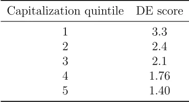
1.5.3 The disposition effect and market capitalization

An important question which will be addressed in this and subsequent sec-tions is whether the DE affects different types of stocks to different extents. Market capitalization, or cap-size, is an important stock-level characteristic and is the primary way that stocks will be categorised in this section. In-vestors in the LDB dataset tilt their portfolios towards stocks with small cap-size relative to a value-weighted market portfolio, as found in Barber and Odean (2000). But a great majority of their positions are still in large cap stocks, by both count and dollar value.

(45)

Capitalization quintile DE score

1 3.3

2 2.4

3 2.1

4 1.76

[image:45.612.213.398.122.222.2]

5 1.40

Table 1.1: Disposition effect score for positions in stocks which are in each capitalization size quintile. Quintile 1 contains stocks with the lowest capi-talization sizes and quintile 5 those with the highest.

the next quintile and roughly halves thereafter for each remaining quintile. Any aggregate pattern such as the DE will therefore mostly be due to what investors are doing with their positions of large cap stocks.

A DE score can be calculated for each cap-size quintile by summing the DE components recorded for positions in stocks that are in that quintile. The results of these calculations are shown in table 1.1. There is a clear decrease in DE as cap-size increases, with the smallest stocks in terms of cap-size having a DE that is twice that of the largest cap-size stocks. This result is in agreement with those in Kumar (2009b), which show that more volatile stocks tend to have a stronger DE as a group, and volatility decreases with cap-size. These results and those of Kumar both contradict an earlier paper on the topic by Ranguelova (2001), which also uses the LDB dataset and finds the exact opposite: that the DE is stronger for stocks with larger cap-size. An Odean-type score was used there too, but with some different choices made about what exactly is counted. However, an attempt to follow the methodology set out by Ranguelova as closely as possible still produced the same result, that the DE is weaker for larger cap-size stocks. The reason for the discrepancy remains unknown.

(46)

[image:46.612.145.471.252.507.2]

(47)

[image:47.612.126.470.297.554.2]

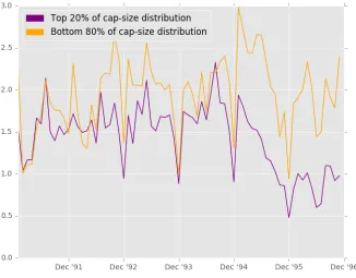
cap-size quintile and one for the other 80% of stocks grouped together. The series for the largest cap-size quintile is essentially the same as the series for all stocks in figure 1.1. But the DE score for smaller cap stocks is consistently higher, most notably in the last two years. Although there is a fall starting in mid ’95 that mirrors that of the largest cap-size quintile, it was at an unusually high level at the start of the year and rebounded to a level comparable with the rest of the series in ’96, whereas the large cap series stayed low.

Figure 1.6: The number of sales for a gain and a loss each month across all stocks in the bottom 80% of the cap-size distribution.

(48)

[image:48.612.120.471.255.517.2]

(49)

group. Figures 1.6 and 1.7 show the corresponding series for the smaller cap group. Breaking it down into these components reveals that the DE score for small cap stocks is generated in a different way to the large cap group. The number of sales for a gain and a loss are much closer together throughout the period, hence for there to be a DE > 1 the number of opportunities to sell for a loss has to be much larger than the number of opportunities to sell for a gain. The second figure shows that this is indeed the case; there is a fall in the number of loss days during ’95, as there is in the aggregate series, but even then it remains higher than the number of gain days. This is a good example of something that would not be apparent looking only at the DE score by itself.

1.5.4 The influence of individual stocks on the

aggre-gate disposition effect

Given that there is a DE in aggregate across all stocks, a next step is to investigate the relative importance of individual stocks in producing the aggregate effect. The component counts due to an individual stock, which will be referred to as the stock-specific components, can be summed across investors and used to quantify the effect that trades of the stock have on the aggregate DE.

Measuring influence

The statistical concept of influence can be used to do this, where the param-eter estimate is calculated with and without the observation in question and the two resulting estimates are compared.12 In this case, the aggregate DE score is recalculated after subtracting the stock-specific components from

12_{The formula used here is the same as the DFBETA measure of influence commonly}

(50)

the aggregate totals e.g. the number of times the stock was sold for a gain is subtracted from the total number of realized gains across all stocks. The new DE score is then subtracted from the original, giving a measure of the stock’s total effect on the aggregate DE. This will be referred to as the stock’s influence on the aggregate DE, or DE influence. Recalling the for-mula for the DE score given in 1.3, the DE influence for a stock indexed by j is defined as

IFj =DE−DE−j

whereDE is the aggregate score across all stocks andDE−j is the same score

calculated without the component counts contributed by stockj. A positive value of DE influence means the stock makes the aggregate score larger; a negative value means it makes it smaller. Such stocks will be labeled DE strengthening and DE weakening respectively.

The distribution of influence across stocks is extremely uneven, and is es-sentially zero for the majority of the 9,812 stocks traded in the dataset. The most common reason for a stock to have near-zero influence is a low number of positions of that stock. As noted in section 1.5.3, investment value is highly concentrated in a small number of large cap-size stocks, with a long tail of smaller stocks that relatively few investors hold. For stocks with few positions, subtracting their component counts from the aggregates will not change the DE score much, regardless of the ratios of the stock-specific com-ponents. There will also be some stocks with a large number of positions whose component ratios closely match the aggregate ratios, and hence will have an influence close to zero.

(51)

[image:51.612.119.488.244.505.2]

ex-tremes of the distribution, essentially reaching zero by the 10th and 90th percentiles. Much of the decay happens within the first and last percentiles. If stocks with influence scores in the top 1% are removed, the aggregate DE score falls by 15%, and if the bottom 1% are removed, it increases by 17%.

Figure 1.8: Plots of the bottom (left) and top (right) 10% of DE influence scores across all stocks.

(52)

three groups will be referred to as DE strengthening, DE weakening and DE neutral. The decay in influence is smooth at both the top and bottom of the distribution, hence changing the cut-off percentiles does not significantly alter the rest of the analysis.

Capitalization and volatility

First the composition of each influence group in terms of market capital-ization and volatility will be examined. Annual cap-size and volatility data were obtained from the CRSP stock files, and quintile groups defined for each of the two variables in the same way as before. As with cap-size, the volatily quintile a stock is assigned to is updated annually using the returns data for the previous year.

For each year, the DE influence for each stock is calculated using the stock-specific and aggregate components for that year. Stocks are then assigned to one of the three influence groups by splitting them at the 5th and 95th percentiles of the year’s influence score distribution. This generates an an-nual sequence of DE influence groups that a stock is part of during the data period. Given that there are 9,812 stocks for which DE components can be counted, every year the DE strengthening and DE weakening groups will both contain 982 stocks, and the DE neutral group will contain 7,848.

Along with the influence group, the stock’s cap-size and volatility quintiles are also recorded for each year. Across all stock-year observations which are in a particular influence group, the percentage which were in each quintile at the time can be calculated. Table 1.2 gives these percentages for each combination of influence group and cap-size quintile. The stocks with the smallest cap-sizes are in quintile 1 and the largest are in quintile 5.

(53)

Cap quintile DE Weakening % DE Neutral % DE Strengthening %

1 1.68 19.98 3.95

2 3.57 21.69 9.33

3 9.87 20.96 17.23

4 20.83 20.28 25.33

5 64.04 17.09 44.16

Table 1.2: Percentage of stock-year observations belonging to each DE in-fluence group where the stock was in a certain cap-size quintile, for each of the five quintiles. Note that the columns sum to 100 (with some allowance for rounding), but the rows do not. This is because the quintiles are defined based on all stocks in the CRSP database and hence the distribution across quintiles of stocks traded in this dataset does not need to be even.

Stock-year observations in the DE strengthening group are also concentrated in the larger cap-size quintiles, but to a lesser extent. Whilst large cap stocks have a lower DE as a group, there is clearly an important subset that have high influence and make the aggregate DE stronger. This would not be evident when looking only at individual stock DE scores, or aggregate scores for cap-size groups. In contrast to the high influence groups, the DE neutral observations are distributed evenly across all cap-size quintiles. This confirms that as well as low cap-size stocks with few positions, there are also large cap stocks with low influence due to the ratios of their component counts being close to the aggregate values.

(54)

Volatility quintile DE Weakening % DE Neutral % DE Strengthening %

1 29.76 16.83 7.95

2 27.22 19.36 13.78

3 21.15 21.29 18.47

4 14.83 21.56 31.18

5 7.03 20.97 28.62

Table 1.3: Percentage of stock-year observations belonging to each DE in-fluence group where the stock was in a certain volatility quintile, for each of the five quintiles. Note that the columns sum to 100 (with some allowance for rounding), but the rows do not. This is because the quintiles are defined based on all stocks in the CRSP database and hence the distribution across quintiles of stocks traded in this dataset does not need to be even.

present in the largest cap-size quintile. The distribution across quintiles is again very even for the DE neutral group, reflecting the much wider cross-section of stocks which are in this group at any time. As in Section 1.5.3, these results again provide support for the finding in Kumar (2009b) that stocks with greater volatility have a stronger DE.

Changes from year to year

(55)

1st group → 2nd group % of observations

S →W 0.59

S → N 2.04

S →S 2.38

N → W 2.05

N →N 85.9

N → S 2.04

W →W 2.36

W → N 2.06

W → S 0.58

Table 1.4: The percentage of pairs of consecutive years for all stocks (49,060 in total), where the stock was in two particular DE influence groups across the two years, for all combinations of influence groups.

Table 1.4 shows the percentage of all pairs of years per stock, 49,060 in total, with each influence group combination. Each influence group is abbreviated to its first letter, so for example S → N indicates the stock was in the DE strengthening group in the first of the two years, and in the DE neutral group the second. W→W indicates that the stock was in the DE weakening group in both years. These results confirm that there is significant movement between the neutral group and the two high influence groups, and even some very large jumps between the strengthening and weakening groups.

(56)

1st group → 2nd group Mean volatility change % Mean cap-size change %

S → W -7.44 29.87

S→ N -4.92 28.4

N →W -1.11 32.5

S → S 0.01 28.34

W→ N 0.12 11.29

W → W 0.66 16.0

N → N 1.06 37.09

N → S 4.1 36.06

W → S 8.52 10.52

Table 1.5: The mean change in cap-size and volatility for stocks in two particular DE influence groups across two years, for pairs of consecutive years across all stocks.

the strengthening straight to the weakening group also have the largest fall in mean volatility.

At the other end of the table, the two group combinations with the greatest increase in mean volatility are those where stocks move closer to the DE strengthening end of the distribution, with the stocks making the largest move again having the largest increase in volatility. Stocks moving from the weakening to the neutral group also have a positive mean change in volatility, but it is smaller and comparable with stocks that stay in the same group, who all have small but positive changes in volatility.

(57)

to switch to the DE strengthening group.

1.5.5 Summary

Existing work on individual investor trading behaviour tends to look only at the disposition effect and the factors affecting it in cross-section, and aggregated over a large number of investors or stocks. By decomposing the aggregate DE into its component parts, this section has been able to establish how the different parts interact to create changes in the DE over time. The fall in aggregate DE during ’95 and ’96 is driven by a dramatic decrease in the number of opportunities to sell stocks for a loss at the time. This in turn is due to the strong performance of the stock market in ’95 and ’96, the start of a boom that culminated in the dotcom crash. Despite the fall in the number of opportunities to sell for a loss, investors still chose to sell a similar number of stocks for a loss as in previous years, likely due to the desire to offset capital gains and reduce their tax burden. Hence the proportion of losses realized increased and the disposition effect fell.

Looking at time series of the different component parts also revealed a dif-ference between the largest 20% of stocks in terms of market capitalization, and those in the rest of the distribution. This large cap group had a lower DE than the rest of the stocks for most of the data period, but with consis-tently more sales for a gain than for a loss. In contrast the smaller cap group had roughly equal numbers of sales for a gain and a loss each month. The lower DE for the large cap group is produced by the much greater number of opportunities to sell these stocks for a gain than for a loss; the opposite was true for the smaller cap stocks with many more opportunities to sell for a loss in most months.

(58)

zero influence. Most of these high influence stocks are in the largest 20% of stocks in terms of cap-size due to these stocks being by far the most commonly held in the dataset. This shows that whilst smaller cap stocks have a higher DE as a group, it is in fact a small number of stocks in the large cap group that increase the aggregate DE by the greatest amount.

Looking at these high and low influence groups over time has shown that stocks do move between them from year to year. Stocks which move closer to the DE strengthening end of the distribution exhibit an increase in volatility, whilst stocks which move in the opposite direction exhibit a decrease.

1.6 The Cox model in detail

The count-based measure of the DE used in the preceding sections was useful for exploratory purposes and detecting aggregate patterns in the data. But to formally test the effect of a covariate on the DE, whilst controlling for the effect of others, a regression model is the best option. Proportional hazards (PH) regression models are preferred to other models such as linear or logistic regression, due to the reasons described in section 1.3.2. Hypothesising the presence of a DE is a claim about the rate at which positions are sold, specifically that gains are sold at a greater rate than losses. Hence modelling this rate directly, as is done in a PH model, will provide a better framework for testing claims about the DE. This section will introduce the Cox model, a particular type of PH model, and discuss its use for measuring the DE.

(59)

λ(t, X(t)) = lim

h↓0

P(t 6T < t+h|T >t, X(t))

h

where T is the time at which the stock is sold. The hazard function is therefore approximately the probability of the stock being sold in the in-finitesimal period of time immediately after t, conditional on the stock not having been sold prior to t and on the ’history’ of the covariates during the period [0, t].

Proportional hazards (PH) models assume that the hazard rate can be split into two components. The first, called the baseline hazard function, is com-mon to all positions and depends only on time. The second depends on the current values of the covariates, which may themselves depend on time. The key assumption of PH models is that changes in the covariates have a multiplicative effect on the baseline hazard, and that this effect is constant over time. Checking this assumption will be an important part of the anal-ysis presented below. In such models, the hazard function can be written as

λ(t, X(t), β) =λ0(t) exp(β>X(t)) (1.4)

where λ0(t) is the baseline hazard function, and β is a p-dimensional vector