Weak factor model in large dimension

(1)

University of Warwick institutional repository: http://go.warwick.ac.uk/wrap

A Thesis Submitted for the Degree of PhD at the University of Warwick

http://go.warwick.ac.uk/wrap/69442

This thesis is made available online and is protected by original copyright.

Please scroll down to view the document itself.

(2)

Weak factor model in large dimension

by

Quang Phan

March 21, 2015

Thesis submitted in partial fulllment of the requirements for the

degree of

Doctor of Philosophy

(3)

List of Figures

2.1 Estimated factor errors vs. pervasiveness (1 corresponds to strong factors) . . . 44 2.2 Estimated factor errors standard deviation vs. pervasiveness (1

cor-responds to strong factors) . . . 44

4.1 ˜

Σk,τu −Σu

,k= 1 : 20for 20 dierent strong factor models,T = 200,

N = 200 andr = 10 . . . 93

4.2 ˜

Σk,τu −Σu

, k = 1 : 20 for 20 dierent mixture strong and weak

factor models, T = 200, N = 200 and r = 10, in which the rst 4 factors are strong (γ = 1₅). . . 94 4.3

Σ˜

k,τ u −Σu

, k= 1 : 20 for 20 dierent weak factor models (γ = 1 5),

(7)

List of Tables

3.1 Strong and weak factors (m= 2, r= 5, γ =1_/₃),_kmax_{= 8}, (_α₌_β ₌

0). The number of factors reported is averaged out of 500 simulations,

on the right side are the standard deviations. . . 63

3.2 Strong and weak factors (m = 2, r = 5, γ = 1_/₃), _kmax _{= 8}, (_α ₌

β = 0.5). The number of factors reported is averaged out of 500

simulations, on the right side are the standard deviations. . . 64

3.3 Strong and weak factors (m= 2, r= 5, γ =1_/₅),_kmax_{= 8}, (_α₌_β ₌

0), the number of factors reported is averaged out of 500 simulations,

3.4 Strong and weak factors (m= 2, r= 5, γ =1_/₅),_kmax_{= 8}, (_α₌_β ₌

0.5), the number of factors reported is averaged out of 500 simulations,

3.5 Strong and weak factors (m = 2, r = 5, γ = 1_/₁₀), _kmax _{= 8},

(α = β = 0), the number of factors reported is averaged out of 500 simulations, on the right side are the standard deviations. . . 65

3.6 Strong and weak factors (m = 2, r = 5, γ = 1_/₁₀), _kmax _{= 8},

(8)

List of Tables

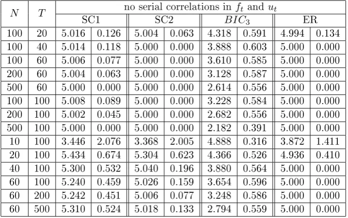
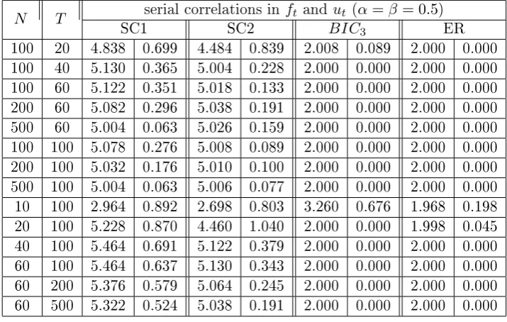
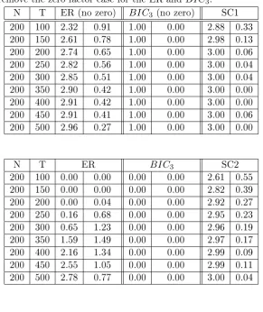
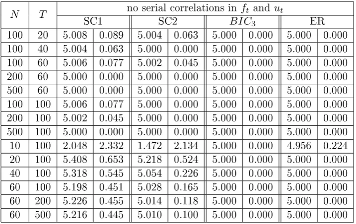
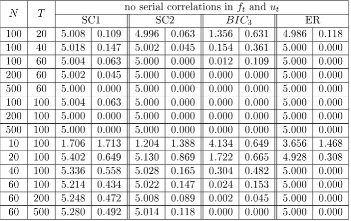
3.7 Regional factors, r= 3, no serial correlations inftand ut,kmax= 8,

the number of factors reported is averaged out of 500 simulations, on the right side are the standard deviations. We also include the case where we remove the zero factor case for the ER and BIC3. . . 67

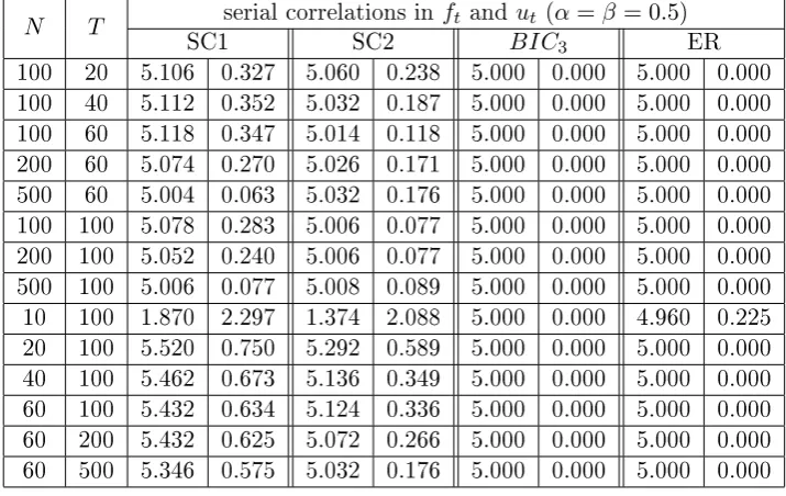
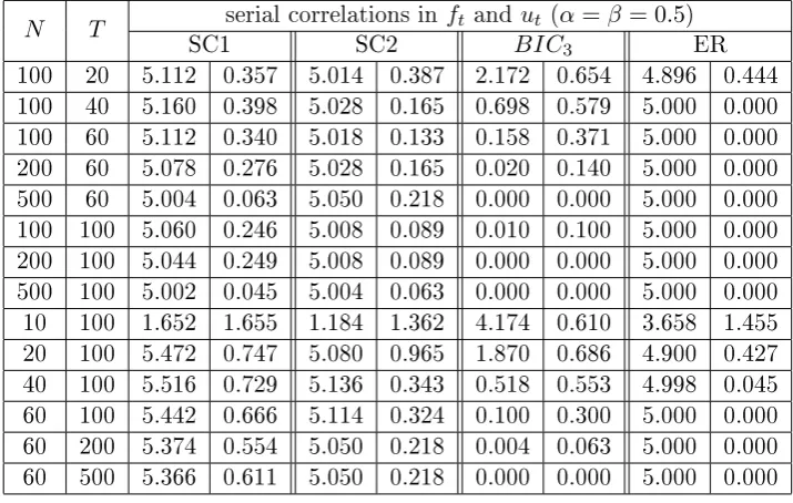
3.8 Regional factors, r= 3, with serial correlations inft andut (α=β =

0.5)kmax= 8, the number of factors reported is averaged out of 500

simulations, on the right side are the standard deviations. We also include the case where we remove the zero factor case for the ER and

BIC3. . . 68

3.9 Strong factors only (r = 5), kmax = 8, (α =β = 0), the number of factors reported is averaged out of 500 simulations, on the right side are the standard deviations . . . 83

3.10 Strong factors only (r = 5), kmax= 8, (α=β = 0.5), the number of factors reported is averaged out of 500 simulations, on the right side are the standard deviations . . . 84

3.11 Weak factors only (r = 5, γ = 1_/₃), _kmax _{= 8}, (_α ₌ _β _{= 0}), the

number of factors reported is averaged out of 500 simulations, on the right side are the standard deviations . . . 84

3.12 Weak factors only (r = 5, γ = 1_/₃), _kmax _{= 8}, (_α ₌ _β _{= 0}_.₅), the

3.13 Weak factors only (r = 5, γ = 1_/₅), _kmax _{= 8}, (_α ₌ _β _{= 0}), the

3.14 Weak factors only (r = 5, γ = 1_/₅), _kmax _{= 8}, (_α ₌ _β _{= 0}_.₅), the

(9)

List of Tables

3.15 Weak factors only (r = 5, γ = 1_/₁₀), _kmax _{= 8}, (_α ₌ _β _{= 0}), the

number of factors reported is averaged out of 500 simulations, on the right side are the standard deviations . . . 86 3.16 Weak factors only (r = 5, γ = 1_/₁₀), _kmax _{= 8}, (_α ₌ _β _{= 0}_.₅), the

5.1 Some criteria for each observed factor model . . . 103 5.2 Number of latent factors suggested by dierent criteria . . . 103 5.3 Sparsity levels and sparsity criterion after each number of factors

(10)

Acknowledgment

Completing the PhD is indeed a fascinating journey. Looking back at the whole period, I have realised many parts of me have changed in a positive way from the date I started the journey. Days and nights of thinking about my research questions and sitting in front of a screen writing up my solutions for these open-ended questions surely will have big impacts for my future career as a researcher.

This completion will start a new chapter of my life and I am obliged to express my special thank to all the people who have been by my side and supported me in this fascinating journey.

First of all, I can not express how grateful I am to my supervisor, Prof. Corradi, for her great support throughout my whole PhD period. She is the best mentor that I could ever ask for, both academically and personally. None of the results in this thesis would happen without her great comments and feedback.

Also, I really appreciate the Department of Economics at Warwick for letting me into the PhD program and provides very generous supports in my 4 years completing this thesis.

Some results in this thesis are obtained based on some advices and comments from Yuan Liao, Chris Heaton, Mike Pitt, and my brother-in-law Long Tran Thanh. Thank you for bringing such insightful and valuable ideas that contribute toward the results in here.

(11)

List of Tables

(12)

Declarations

(13)

Abstract

This thesis presents some extensions to the current literature in high-dimensional static factor models. When the cross-section dimension (represented by N hence-forth) is very large, the standard assumption for each common factor is to have the number of non-zero loadings grow linearly withN. On the other hand, an idiosyn-cratic error for each component can only be correlated with a nite number of other components in the cross-section. These two assumptions are crucial in standard high-dimensional factor analysis, as they allow us to obtain consistent estimators for the factors, the loadings and the number of factors. However, together they rule out the possibility that we may have some factors that have strictly less than N but still non-negligible number of non-zero loadings, e.g. Nα for some 0 < α < 1. The existence of these weak factors will decrease the signal-to-noise ratio as now the gap between the systematic and idiosyncratic eigenvalues is more narrow. As the consequence, in such model it is harder to establish the consistency of the factors estimated by sample principle components. Furthermore, the number of factors is even more challenging to identify because most existing methods rely on the large signal-to-noise ratio. In this thesis, I consider a factor model that allows general strength for each factor, i.e. both strong and weak factors can exist. Chapter 1 gives more discussions about the current literature on this and the motivation for my contribution.

(14)

List of Tables

not too weak. In addition, I derive the lower bound that the strength of the weakest factor needs to achieve for being consistently estimated. More precisely, what I mean by strength is the order of the number of non-zero loadings of the factor.

Chapter 3 presents a novel method to determine the number of factors, which is asymptotically consistent even when the factors are weak. I run extensive Monte Carlo simulations to compare the performance of this method to the two well-known ones, i.e. the class of criteria proposed in Bai and Ng (2002) and the eigenvalue ratio method in Ahn and Horenstein (2013).

(15)

1 Introduction

Factor analysis rst arises in the eld of Psychometrics, when Spearman (1904) obtained results of several tests taken by schoolchildren and proposed that the cor-relations between those tests were due to a single factor, which he referred to as intelligence. Since then, there has been a rapid growth in applications of factor anal-ysis in social science, particularly in Finance and Economics. It is very useful and interesting to nd a small number of factors (either observed or unobserved) that capture the movements of a much larger number of variables. For examples, Boivin et al. (2013) address a strong factor, can be interpreted as credit shock, which has big impacts on several other nancial and economic variables such as credit spreads, interest rates, etc. Additionally, from the statistical angle identifying the common factors brings a great advantage of dimension reduction in the large-dimensional setting.

In this thesis, I focus on the case where factor model is used as a dimension reduction technique. For example, in some applications such as estimating large covariance matrix or forecasting with many explanatory variable, the factors after extracted are used in place of the original components. Therefore, this gains benet of reducing the dimension signicantly.

(16)

1.1 Literature review

consistency of the factors estimated by the standard principle components technique. In addition, changing this assumption also has some impacts for other areas of re-search regarding factor analysis, such as determining the number of factors and the estimation of covariance matrix using factor analysis. Therefore, other contributions in this thesis are about determining the number of factors and applications of factor analysis in computing the large covariance matrix.

The main contributions here belong to the theory of Econometrics, rather than Economics empirical ndings. Therefore, discussions and application of the common factors identication are mainly approached from a statistical point of view. I do not focus on the case where there is a need to interpret the meaning of the underlying factor processes.

In contrast, there are many other empirical works exploiting factor analysis and interpret the factors as some meaningful variables for insights. Examples within this line of research including studies regarding identifying the factors (or shocks) in yield curve (Diebold et al. (2006)), stock returns (Fama and French (1993)), credit market (Boivin et al. (2013), Gilchrist et al. (2009), etc.), credit default swaps (Chen and Härdle (2012)), corporate bond spreads (Elton et al. (2001)), etc. Nevertheless, the centre of discussion in this thesis regarding general factor identication issues in large-dimensional setting, rather than these nancial and economic applications.

Over the next few sections in this chapter, I will gradually discuss some recent rel-evant advances in factor analysis. Also, some applications are mentioned to illustrate how this can be used in practice.

1.1 Literature review

(17)

1 Introduction

1.1.1 Developments in factor analysis

Since the literature is extremely large, it is impossible to present all the important related works in the review, hence there are many signicant results missing in these subsequent sections. For example, I will not discuss dynamic factor model in details despite its importance, because static factor is the main focus of this thesis. In contrast, some results in the large covariance matrix estimation will be mentioned, due to its link with the main contribution.

1.1.1.1 Overview of factor analysis

In particular, a static factor model foryit, i= 1, ..., N is given by:

yit=λ(1)_i ft(1)+...λ

(r)

i f

(r)

t +uit. (1.1)

or

yit =α+λ0ift+uit. (1.2)

where λi = [λ(1)_i , ..., λ_i(r)]0 is the factor loadings vector for component yit, ft =

[f_t(1), ..., f_t(r)]0 is the common factors vector, uit is the idiosyncratic error (shock)

which is not explained by the common factors. The λi term corresponds to the

exposure ofyit to the common factorsft. In vector form, we can write:

Yt= Λft+ut.

(N×1) = (N ×r)(r×1) + (N×1)

(1.3)

In here, Yt = [y1t, ..., yN t], Λ = [λ1, ..., λN] is the matrix of factor loadings and ut

is the vector of idiosyncratic errors. W.l.o.g we assume that Yt, ft and ut all have

(18)

be written as:

Y =FΛ0+U.

(T×N) = (T ×r)(r×N) + (T×N)

Recently there has been a rapid growth in applications of factor analysis for social science, particularly in Economics and Finance. This is due to the need to seek for a small set of factors that can contain a large proportion of information from the vast original multivariate series. Some well-known examples of factor model in economic theory are the capital asset pricing model (CAPM, Sharp (1964)) and the arbitrage pricing theory (APT, Ross (1976)).

The factor model in Ross (1976) is referred to as strict factor model because it assumes the common factors capture all the correlations between all variables, which means Σu ≡ cov(ut) is a diagonal matrix. However, this assumption may

be too stringent in practice and we normally need to allow for some level of cross-section correlations between the idiosyncratic errors. Therefore the approximate factor model of Chamberlain and Rothschild (1983) seems more appropriate. In this model, the key assumption is that the idiosyncratic covariance matrix is not diagonal, but its eigenvalues must be bounded as N → ∞. I will come back to this in more

details in some later paragraphs.

(19)

1 Introduction

(e.g. principle component (PC) analysis, maximum likelihood estimator, etc.).

Another aspect that plays an important role in theoretical and empirical work is to determine the number of factors in the model. A few methods have already been proposed and used in applications. The simplest method is to select the number of factors from the scree plot of the descending sample eigenvalues of Σ ≡ cov(Yt)

(i.e. eigenvalues of the sample covariance matrix ofYt) as in Cattell (1966). Related

procedures are suggested by Onatski (2009, 2010) using the slope of the scree plot and the dierence of ordered sample eigenvalues, respectively. In addition to these, Ahn and Horenstein (2013) consider maximising the ratio of successive eigenvalues or their growth ratio.

Information criteria have also been used to select the number of factors. Choi and Jeong (2013) study the consistency of using AIC, BIC or HQIC in choosing the true factor model. In addition, Bai and Ng (2002) propose several criteria for the number of factors in approximate factor models and show them to be consistent. The relationship between the information criteria and those based on eigenvalues is discussed in Onatski (2010) and Ahn and Horenstein (2013). Once the number of static factors is determined, the number of dynamic (or primitive) factors can be determined using methods proposed by Amengual and Watson (2007), Bai and Ng (2007), and Breitung and Pigorsch (2012).

This is also worth mentioning at this stage that there can be two dierent ways when specifying the model in (1.2). In the rst one, the common factors are assumed to aect most components in the cross-section, which is called pervasiveness. This formally means the number of non-zero loadings for each factor needs to grow with

N. Literature for this model can be founded in Bai (2003), Stock and Watson (2002),

(20)

assume there is a set of common factors that account for all the serial correlations and hence the idiosyncratic components are just white noise. Some attempts in this direction include Anderson (1963), Priestley et al.(1974), Brillinger (1981), Peña and Box (1987), and Pan and Yao (2008). More recent eorts focus on the inference when the dimension of time series is as large as or even greater than the sample size; see, for example, Lam, Yao and Bathia (2011), Lam and Yao (2013) and the references within. In summary, the rst class of model assumes the common factors leave very little cross-section correlation in the idiosyncratic components but allow for serial correlation, whereas the second class assumesutis serially uncorrelated but

the factors can be less pervasive.

In this thesis, I mainly focus on the static factor model as shown in (1.3) and I adopt the model setup similar to the one discussed in Bai and Ng (2002), Bai (2003) or Stock and Watson (2002), in whichutis allowed for serial correlation. However, as

we shall see, I relax the pervasiveness condition that usually comes with the model.

1.1.1.2 Factors identication

It is very important to notice that the latent factors can not be uniquely identied without further restriction. For example, we can always linearly transform ft and

Λ by an r×r invertible matrix and its inverse and they still generate exactly Yt.

Therefore, we can only estimate the loadings and the factors up to their spanning spaces without any restrictions.

If ft is a stationary process, a well-known restriction is that Σf ≡cov(ft) = Ir,

whereIris ther×ridentity matrix. This is simply done by replacingftbyΣ−_f1/2ft.

However, this is still not sucient for unique identication, because for now we can still rotate the factors by an orthonormal matrix and still having cov(ft) = Ir.

(21)

1 Introduction

of them, without loss of generality because we know that any other restrictions can be retrieved by a linear transformation. These restrictions are often found in the maximum likelihood estimation, e.g. see Lawley and Maxwell (1971). Furthermore, as discussed in Bai and Ng (2013), it is not as stringent as it seems, and can be useful for economics applications. An example shown in Bai and Ng (2013) is the case wherer= 3 and

Λ = 

    

Λ1 0 0

0 Λ2 0

0 0 Λ3 

    

(1.4)

where Λi is the Ni ×1 vectors of loadings, and N1 +N2 +N3 = N. This model

implies that the rst factor generates the rstN1 group of cross-section components,

and so on. This can be applied in models for regional panel data. Even when the order of the cross-section components is shued, the loadings matrix restriction still holds, which makes it useful because we do not require the knowledge of the grouped structure. In this thesis, these restrictions regarding the factors and loadings are not needed for the main results, although I shall often refer to this restriction in some discussions for convenience.

Having discussed about estimators for the factors and the loadings matrices, it is also important to point out that in large dimensional setting (N is as large as T), principle components (PCs) analysis is considered as the most ecient methods to achieve this task. The rstr (population) PCs of Yt, denoted as gt, are dened as

follows:

gt=B0Yt

whereBis theN×rmatrix whose columns consisting ofreigenvectors corresponding to ther largest eigenvalues ofΣ, normalised so thatB0B =Ir. We can also write:

(22)

withE(gtw0t) = 0. Intuitively, if the rstr principle components already capture the

large proportion of variation inYt, the termwtcan be interpreted as the disturbance.

Therefore, as in (1.3) and (1.5) there is a similarity between the PCs and factors. In fact, Schneeweiss (1997) develops a result which shows the convergence of PCs to the factors. The key requirement for this convergence is:

µr(Λ0Λ)

µ1(Σu)

→ ∞. (1.6)

whereµk(A) is the kth-largest eigenvalues of a square matrixA. The ratio in (1.6)

can be interpreted as the signal-to-noise, and is a key parameter that determines how well one can identify the factors.

The results in Schneeweiss (1997) are developed for population PCs, where Σ is assumed to be known. However, replacing Σ by the sample covariance matrix introduces further sampling errors, especially when N is large. The convergence of sample PCs to factors space is one of the crucial developments recently, and can be found in Bai (2003), Bai and Ng (2002) or Stock and Watson (2002). The authors show that when (N, T) → ∞, the sample PCs converge to the factors space under

some conditions, in which some among them imply (1.6).

In order to get to our main contribution, it is worth explaining the intuitive inter-pretation behind the seemingly technical condition (1.6). Whatµ1(Σu)andµr(Λ0Λ)

represent are really the amount of cross-section correlations in the idiosyncratic com-ponents and the pervasiveness of the factors. First we discuss about Σu, which was

originally assumed to be diagonal in Ross (1976). However, since the introduction in Chamberlain and Rothschild (1983), the idiosyncratic errorsuit are allowed to be

cross-sectionally correlated, i.e. we can have a pair (i, j) such that cov(uit, ujt)6= 0.

This is called approximate factor model, as opposed to the strict factor model where cov(uit, ujt) = 0 for all i 6= j. Although allowing Σu to be dierent than a

(23)

1 Introduction

asN → ∞.

In this case, if the factors are pervasive enough, then (1.6) is satised. To see why, the pervasive condition is usually stated as: PN

i=1

λ(_ik)2 grows linearly withN for any k ∈ (1, ..., r). Equivalently, for any factors, the number of non-zero loadings must grow strictly with orderN. IfΛ0Λis a diagonal matrix as usually assumed for unique identication, then the eigenvalues lie on the diagonal, and thekth eigenvalue is PN

i=1

λ(_ik)2. So condition (1.6) is satised if the factors are strongly pervasive andµ1(Σu) is bounded.

These two conditions regarding low cross-section correlations of idiosyncratic errors and pervasiveness of factors can be founded in most recent works of factor models such as in Bai and Ng (2002), Bai (2003), Stock and Watson (2002) and the references therein. For example, I recall the two assumption B and E2 in Bai (2003) and denote them as Assumption 0 in this paper:

Assumption 0. (i)Λ0Λ/N converges to a positive denite matrix Dwhose eigen-values are bounded away fromboth 0 and innity

(ii) Σu has bounded row sum of absolute entries, i.e. maxiPj|σij|=O(1) where

σij =cov(uit, ujt).

Assumption 0 (i) makes sure that each factor has impacts on the majority of the components in the cross-section. Assumption 0 (ii) describes the level of cross-section correlations between the idiosyncratic errors. Slightly weaker one is used in Bai and Ng (2002): 1

N

P

i

P

j|σij|=O(1). The main idea behind these restriction onΣu is

that although the model allows for approximate factor, the level of correlations across the idiosyncratic errors can not exceed a certain level. Notice that if|σij|is bounded

(24)

To see why, notice that:

max

i

X

j

I{|σij|>0}= max i

X

j

|σij|0I{|σij|>0}

= max

i

X

j

|σij|(|σij|)−1I{|σij|>0}.

≤max

i,j

(|σij|)−1I{|σij|>0}

max

i

X

j

|σij|=O(1).

Intuitively, maxiP_jI{|σij| > 0} = O(1) means that the number of non-zero

entries in each row of Σu must be bounded while its dimensionN grows to innity.

Therefore, later on we will use the fact that maxiP_jI{|σij| > 0} = O(1) can be

derived from of Assumption 0 (ii)1_{. The reason for looking at}_max_iP

jI{|σij|>0}

is that we want to use some important results in the sparse matrix2 _{literature. This}

is useful for us later to construct a method to estimate the number of factors (see Chapter 3).

In addition, Assumption 0 (ii) implies that µ1(Σu) is bounded3. Therefore,

to-gether conditions (i) and (ii) of Assumption 0 imply (1.6), which contributes to the sucient conditions required for the population PCs to converge to the factors. How-ever, it may be stronger than necessary because we only need (1.6) to hold. It is interesting to consider the cases where Assumption 0 does not hold and examine whether the population and sample PCs still converge to the factors space. Clearly, the sample PCs case will be the ultimate goal, so most of the current studies directly establish the consistency result for this.

One such interesting case is discussed in the PhD thesis of Heaton (2008). This is the case whereP

j|σij|grows with rateN1−αfor someiand0< α≤1. In this case,

Heaton (2008) shows that the sample PCs still converge to the factors, but with a

1_{The condition}_maxi,j

(|σij|)−1I{|σij|>0}=O(1)is reasonable, as it just simply states all the non-zero entries inΣumust be bounded away from 0, which is true whenΣuis non-stochastic.

2_{A large matrix with many zero entries is called sparse matrix, and this has attracted a large}

number of studies recently

3_{As from standard Linear Algebra result, we have}_µ

(25)

1 Introduction

slower rate. Particularly, he proves that (using our notations):

1

T

F˜

r₋_{F A} 2

=Op(

1

Nα +

1

T)

where_F˜r _{is the sample PCs and}_A _{is a rotational matrix. In Heaton's thesis, where}

he assumes the column ofF is orthonormal,A becomes only a signs matrix. Under Assumption 0, the rate of convergence for similar quantity in the left hand side above is established in Bai and Ng (2002) and is Op(N−1 +T−1). Therefore we can see

how weakening Assumption 0 (ii) aects the rate of convergence.

In this thesis, I mainly focus on the case where Assumption 0 (ii) is not violated, but we relax Assumption 0 (i). There are some reasons for this to be too stringent, because under this condition a factor that only aects a relatively small number of cross-section components (sayN2/3 out ofN) will not be assumed to exist. However, recently some empirical works suggest the potential loss of information when ruling out these not-so-strong factors. For example, Boivin and Ng (2001) provide an empirical study illustrating that a smaller but carefully chosen set of cross-section variables yields better factors than the whole original set. One potential reason for this is that the amount of correlations from the large number of idiosyncratic errors will reduce the sharpness of the estimators. In addition, some factors that are extracted from the subset can be identied as idiosyncratic errors when applying factor analysis to the full set, due to their small explanatory powers for the majority of cross-section variables.

(26)

in the middle, that is we assume the number of non-zero loadings for each factor is at order d(N), which can be dominated by N but has to grow to innity with N. We even consider the general case where d(N) varies from factors to factors. This is found useful in the case where some factors are global while some of them are regional, but both the number of regions and the sizes of them can be large.

Another related area of research with weak factors is the multi-level factor model, which usually includes global and regional levels. In such model, the factors are separated into levels, where the top level factors (global factors) are pervasive and aect almost every cross-section component. The second level factors are not as pervasive because they only aect components in each region. In a special case where the number of components in each sector grow at a slower rate thenN, this 2-level factor is a special case of a mixture model of strong and weak factor. Restriction for such model and eective identication method can be found in Wang (2008). The most important similarity between the multi-level factor model and the one presented in this thesis is that the loadings matrix can be allowed to have many zeros. However, there is a key dierence, which is that in my proposed model we neither know how to separate the original cross-section into sectors nor if such separation is possible.

1.1.2 Applications of factor model

There are a wide range of applications of factor model that can be found in the Economics and Finance literature. They can be separated into two classes: the rst one links the factors with some interpretations for meaningful insights about the observed variables (e.g. APT, CAPM, Fama-French 3 factor model, business cycle4_,

yield curve modelling5_{, etc.), whereas the second class uses the factor analysis as a}

tool for dimension reduction. In here, I focus more on the second one.

High-dimensional settings can be found in many applications recently, due to the growth in available data and the advance in computational techniques. Typically

(27)

1 Introduction

the vast dimension can be hundreds or thousands, e.g. number of rms in the stock markets or macro variables in the global economy. An unarguable advantage with the growth in the size of data is to capture more information which can not be revealed from any smaller sets.

However, this clear advantage is not taken for granted, because the suitability of analysis tools used for these large dimensional data has to be examined before being applied. For example, in the case where the number of interested variables expands faster than their sample sizes, many traditional theoretical estimators in data analysis break down due to undesirable bounds required for convergence, such as the sample covariance matrix of these data. Therefore, a large class of innovative methods has arisen which either seek for dimension reducing techniques or extend the theoretical results for large dimension, including factor analysis.

1.1.2.1 Large covariance matrix estimation:

To begin we give one such technically challenging example that arises in high-dimensional setting: i.e. estimating the covariance matrix when the cross-section dimension (N) of the data is as large as the sample size (T). It is well known that in this situation, the sample covariance matrix is very ill-behaved, and it is not even invertible whenN > T. Since the development of Markowitz portfolio theory, covari-ance matrix of returns has been an important concept in Fincovari-ance and Econometrics, and we would denitely want to have a good6 _{estimator for this, no matter how}

largeN is.

For some backgrounds in this area: suppose we have a portfolio ofN assets. Based on Markowitz portfolio theory, nding the optimal portfolio allocation requires us to estimate theN×N covariance matrix across the assets returns (assume constant in this period), denoted Σ. The diagonal of this matrix is the variance of each asset return in the portfolio, where the(i, j)o-diagonal entry is the covariance of returns

(28)

between asset iand asset j. In order to allocate the weighs of investment for these assets within a portfolio, we may choose the one that reaches our required expected return with minimal variance. If we denote Yt = {yit}N_i₌₁ the vector of N assets

returns at timet, the variance of the portfolio with weighsw={wi}Ni=1 is:

var(w0Yt) =w0Σw.

Therefore, it can be seen that the covariance matrix has a closed link with risk management in practice. Solutions for estimating high-dimensional Σ are normally obtained by proposing a structure for the covariance matrix (or in other words, for the data generation process of Yt). This is usually called regularisation. Some popular

regularised restrictions are banded and sparse, which restrict the number of non-zero entries in Σ. However, applying a sparse (or banded) structure directly toΣ is not realistic, for example it is possible that all assets returns are correlated with each other. Therefore a more rational restriction is thatΣcan be decomposed into a sum of a low rank matrix and a sparse matrix, a property that can be resulted if Yt has

a factor structure representation. If (1.2) holds true and ft and ut are independent

then:

Σ = ΛΣfΛ0+ Σu. (1.7)

where Σf and Σu are the covariance matrices of ft and ut. The decomposition in

(1.7) provides an ecient estimator forΣifr is small andΣu has many zero entries.

In this case, the product matrix ΛΣfΛ0 has rank r and Σu is sparse, so we

signi-cantly reduces the number of parameters required to estimate.

(29)

1 Introduction

1.1.2.2 Forecasting with diusion indexes7_:

Assuming we want to forecast ah-step ahead for a variable xt and know that xt+h

can be predicted by the following forecasting model:

xt+h=α+Ft0β+t+h

In this case, although the factorsFtis not observed, it can be extracted from other

observable variables in the market, i.e. Yt if in fact we have a factor structure as in

(1.3). Given that the dimension of Yt (N) is very large, it is desirable to use the

factors as the explanatory variables in the forecasting equation.

1.1.2.3 Large-dimensional vector autoregressive:

Consider a task where one may want to forecast the future values for{yit} for some

i∈(1, .., N). We can imply they follow a VAR structure with some added exogenous

variables. i.e.

Yt= Θ(L)Yt+ ΓZt+t

where Yt = (y1t, ..., yN T), Zt represents the exogenous variables and t consists of

some noises that are spatially uncorrelated. When N is small we can estimate all the unknown parameters by maximum likelihood, as usual. Where N is large, or even extremely large this can yield further problem due to infeasibility to cope with large number of unknown parameters. One way to solve this problem is that we can assumeYthas the factors structure as in (1.3) and replace the Yton the right

hand-side withΛft. After obtaining ft from Yt thenΘ(L)Λ can be estimated together as

a single lag matrix and has much less parameters thenΘ(L). For example, if the lag of our VAR model is 1 thenΘ(L)Λ is a N ×r matrix whereasΘ(L) is theN ×N matrix.

(30)

1.2 Contributions of this thesis

In this thesis, I attempt to replace the strong pervasiveness condition for the factors with a less stringent one, while assuming that the idiosyncratic covariance matrix is sparse. The sparsity of Σu is stated through Assumption 2 (iii), which is same as

Assumption 0 (ii). Particularly, when Σu has bounded row sum uniformly and nite

entries, the number of non-zero entries of Σu must be bounded. This has better

interpretation in some applications, e.g. conditional on the common factors, most asset returns in the market are uncorrelated. I later on dene the sparsity level of a matrix as its maximum number of non-zero entries in a row, and by this denition

Σu must have bounded sparsity level. This fact is also found useful later when a

novel criterion to choose the number of factors is proposed.

In summary, together with the sparsity assumption forΣu, here are some important

questions that are studied in this thesis:

1. If we loosen the restriction thatΛ0Λ/N →DtoΛ0Λ/d(N)→Dfor a function d(N) that grows to innity at a slower rate than N can we still identify the

factors, given that the number of factors is known. Recall from above thatD is a positive denite matrix whose eigenvalues are bounded away from both 0 and innity. Furthermore, replacingN with a single termd(N)means that all the factors still have same strength order. I will also generalise to discuss the case where each factor can have dierent strength, which also generalises the multi-level factors model in Wang (2008). This is described later in Assumption 1.

2. If it turns out that the factors can be identied in the weak factor model but we do not know the number of factors, how do we consistently estimate it?

(31)

ro-1 Introduction

tation matrix which equals (Λ0Λ/N)(F0F˜k/T)(Vk)−1 where F˜k is the matrix of k estimated factor by PCs and Vk is the k×k diagonal matrix of the rst k largest eigenvalues ofY Y0/(N T) in decreasing order. Therefore an important condition is that this rotation matrix has eigenvalues bounded away from both 0 and∞. For the

case when onlyΛ0Λ/d(N)→D, this is not straightforward even whenk is the true number of factors, so it requires further investigation and modication to the work of Bai and Ng.

In addition, most current methods in determining the number of factors such as in Bai and Ng (2002), Onatski (2010), Ahn and Horenstein (2013) exploit the sharp edge in the set of sample eigenvalues of Σ, which separates the factors and the errors. These are all based on Assumption 0 that intuitively states thatΣ has exactlyr spiked eigenvalues growing at rate N. In our setting, because of replacing this crucial condition, the number of factors is now much harder to determined. For example, using the ratio of eigenvectors method of Ahn and Horenstein (2013), there might easily be a case where the ratio of ordersNα and N eigenvalues for α <1 is less than the ratio ofN0 andNα eigenvalues. Clearly, we want the number of factors to be at the point where the eigenvalues of Σ begin to be bounded but it will not always be possible to identify in this case, using the sample eigenvalues ratio based method. In support of our argument, Yu and Samworth (2013) provide some Monte Carlo results that show how the Bai and Ng (2002) criteria can underestimate the number of factors when the rst r largest eigenvalues of the data are not as spiked as rate linear withN.

(32)

1.2 Contributions of this thesis

(33)

2 Factor identication under the

weaker assumption

In this chapter, I discuss the identication of factors under the weaker assumption. It will later be seen that a factor and its loading space are still consistently estimated if the factor has the corresponding number of non-zero loadings more than a certain level. This can be useful for some empirical studies as now we can apply factor analysis to some applications where not all the factors are pervasive. Examples of these situations are the cases where we can have both regional and global factors. If the regional factors are not too weak, we can still extract them from the whole original data set.

First of all, we emphasise thatris xed whileN will grow to innity. The number of factors r includes both the strong and weak factors. We should explicitly clarify here that the nature of our model allows factors with dierent strengths co-exist, hence there must be a clear edge between the weakest factor and the idiosyncratic errors. The fact thatr is xed whenN → ∞is crucial as it implies there must be a

lower bound for the strength of the factors, which leads to the clear edge mentioned previously.

(34)

2.1 Factors identication techniques

2.1.1 Principle Components

The most usual way to estimate the factors and the loadings are via PCA: Given a value for k as a predetermined number of factors, we estimate(Λ, F) by ( ˜Λk,F˜k) such that

( ˜Λk,F˜k) =arg min Λk_,Fk

1

N T

T

X

t=1

(Yt−Λkftk)0(Yt−Λkftk) (2.1)

where Fk = [f₁k0, ..., f_Tk0], f_tk is a k×1 vector representing a factor value at time t and Λk is aN×k loadings matrix. Recently, Choi (2012) and Bai and Liao (2013) generalise the standard PC method to generalised PCA (GPCA) method that gives benet of a lower variance in the estimators, i.e. the objective function becomes:

arg min Λk_,Fk

1

N T

T

X

t=1

(Yt−Λkftk)0W(Yt−Λkftk). (2.2)

In here to keep thing simple all the proofs refer to the traditional PC method, but a generalisation is also possible.

As usual the solution for (2.1) is not unique up a rotation, because clearly if

( ˜Λk,F˜k) is a solution of (2.1) then ( ˜ΛkA,F˜kA0−1) is another solution for any in-vertible k×k matrix A. However, if we uniquely restrict ( ˜Λk,F˜k) so that Λ˜k0Λ˜k is diagonal and_F˜k0_F_˜k_/T ₌_I

k, the following pair of solutions of (2.1) can be used: the

columns of_F˜k_{will contain}√_T _{times the eigenvectors corresponding to the largest}_k

eigenvalues of Y Y0, normalized so that F˜k0F˜k/T =Ik, then Λ˜k =Y0F˜k/T. In this

case, it is easy to check that:

˜

Fk0F˜k/T =Ik; Λ˜k

0

˜

Λkis diagonal. (2.3)

(35)

2 Factor identication under the weaker assumption

scenario, in here we must be careful with which version of estimators to choose. For example consider a pair of solution( ¯Λk,F¯k) where:

¯

Λk0Λ¯k/N =Ik; F¯k

0

¯

Fk/T is diagonal. (2.4)

This is a standard estimator also shown in Bai and Ng (2002) or Bai (2003). The method for nding( ¯Λk,F¯k)is as follow: if we concentrate outFk then the columns of _Λ¯k _{will contain the} √_N _{times the eigenvectors corresponding to the largest} _k

eigenvalues of Y0Y, normalized so that Λ¯k0Λ¯k/N = Ik. Then by standard least

square result, _f¯k

t = ( ¯Λk

0_¯

Λk)−1Λ¯k0Yt = ¯Λk

0

Yt/N. However, when the factors are

weak, it is possible to haveΛ0Λ/N singular, and thereforeΛ¯k_{can not be a consistent}

estimator for any rotations ofΛ.

For that reason, when the factors are not pervasive, it is always better to use

( ˜Λk,F˜k) which satisfy (2.3).

2.1.2 Maximum Likelihood Estimator

Assuming the idiosyncratic errorsutare i.i.d and followGaussian(0,Σu), the

objec-tive function for estimating (F,Λ) using conditional quasi log-likelihood (removing all constant terms, and multiplying by -2) is:

1

N log|det(Σu)|+

1

N Ttr (Y −FΛ

0₎0₍_Y ₋_F_Λ0_)Σ−1

u

(2.5)

This can be shown to be more ecient than the principle components method, for discussion see Bai and Liao (2013) or Choi (2012). For example, Choi (2012) shows that the asymptotic variances of the estimators for (F,Λ) are smaller when using the objective function in (2.5) than those obtained when using the original principle component objective function.

(36)

2.2 Notations

min Λk_,fk t

1

N T

T

X

t=1

(Yt−Λkftk)0Σu−1(Yt−Λkftk) (2.6)

In here, the weighted matrix is Σ−_u1. Notice that in this case GPCA to PCA is an analogy with generalised least square to ordinary least square.

However, this also requires an estimator for Σu. The usual way for obtaining

estimator for Σu is to assume that it is diagonal and its diagonal entries are just the

sample variance of a prior tted factor model. Recently, Bai and Liao (2013) replace the diagonal condition forΣuwith sparsity and use the POET estimator. The general

idea of their approach is to nd the factors and loadings by PCA, then estimateΣu

from the residuals1 _{and plug this estimator of}_Σ_u_{into (2.6) to obtain a better version}

of (F,Λ)estimators.

As already mentioned, GPCA brings some benets of variance reduction of the estimators. Most of the results in this thesis can be extended to this, but I only stay in the PCA framework to keep the process and notation clearer.

2.2 Notations

In here I introduce some notations that are used in from here onward. As mentioned before, let Σ and Σu be the population covariance matrices of Yt and ut. Also, let

σij be the entries of Σu. Furthermore, let Σ˜ and Σ˜u be the corresponding sample

covariance matrices. Clearly, only _Σ˜ _{can be computed from observed data,} _Σ˜_u _is estimated with estimated version of ut, which are the residuals after tting in the

factors.

Furthermore, for a given value of k≤r, dene the following partitions:

f_t(l:k)= (f_t(l), ..., f_t(k))0, F(l:k) = (f₁(l:k)0, ..., f_T(l:k)0)

1_{They also apply a thresholding step after computing the residuals sample covariance matrix, as}

(37)

λ_i(l:k)= [λ_i(l), ..., λ(_ik)]0,Λ(l:k)= [λ₁(l:k), ..., λ(_Nl:k)] For more convenient, I also use these notations:

f_tk =f_t(1:k), Fk=F(1:k)

λk_i =λ(1:_i k),Λk= Λ(1:k)

uk_t =Yt−Λkftk,Σku≡

σk_ij=cov(uk_t)

Those notations above are clearly not dened for k > r, however their estimated version can take any values fork.

We consider estimating the factors by PC analysis, _Λ˜k_,_F˜k _{are already dened in}

(2.1) and (2.3), and we will let all the partitions for _Λ˜k_,_F˜k_{similar to the notations}

for the true ones above. Also, we dene:

˜

u_tk =Yt−Λ˜kf˜tk,Σ˜ku =

1

T

X

t=1 ˜

uk_tu˜k_t0

asut has mean zero.

For a square matrix we will let µi be its ith largest eigenvalues. The matrix

norms we use in this paper are the operator norm and the Frobenius norm, i.e.

kAk=µ1(A0A),kAk_F =trace(A0A) respectively. As a special case, we also denote

vi =µi(Σ)andv˜i =µi( ˜Σ). In addition ifan=O(bn) andbn=O(an)when n→ ∞,

we will writeab. Similarly, replacingObyOp, we can denep in a same manner.

Finally, w.l.o.g we assume all the time seriesYt,ut and fthave zero means.

2.3 Asymptotic results

(38)

2.3 Asymptotic results

pervasive factors conditions. However, we also wish to develop a new method for determining the number of factors in Chapter 3, which makes use of some results in Fan et al. (2011, 2013). For example, the stationary condition in Fan et al. (2013) for all stochastic process is stronger than in Bai (2003), but can be still reasonable in practice. Therefore, in this thesis I adopt the similar set of assumptions as in Fan et al. (2013).

Assumption 1. There exists a matrix DN = diag(d1(N), ..., dr(N)), where for all

1 ≤ i ≤ r, di(N) → ∞ and di(N)/N is bounded away from ∞ as N → ∞, such

that D_N−1Λ0Λ → D and all the eigenvalues of D are bounded away from both 0 and innity.

This assumption above allows for a more general case where all the factors can have dierent strengths, which are indicated by the order of di(N). If we assume

Λ0Λ is diagonal, another way to state this assumption is Λ(k) 2

=PN i=1(λ

(k)

i )2

dk(N). In addition, to label the factor according to their strengths, we further let

d1(N) ≥ ... ≥ dr(N) as N → ∞. Recently, Lam et al. (2011) and Lam and Yao

(2012) consider weak factors similar to the ones discussed in this paper. However, there is a key dierence with their factor model, which is assumed to capture all the serial correlation in the original time series. This paper considers a factor model that is similar to the one discussed in Bai and Ng (2002), Bai (2003) or Stock and Watson (2002).

Assumption 2. (i) {ut, ft} is strictly stationary with zero mean and {ft} is

inde-pendent of {ut}.

(ii) 1

T

PT

t=1ftf 0

t → Σf as T → ∞, with µ1(Σf) and µr(Σf) are bounded away

from both 0 and ∞.

(iii) Σu has bounded row sum of absolute entries, i.e. maxiP_j|σij|=O(1).

(iv) (exponential-type tails) There exists constants r1, b1 > 0 such that for any

s >0 andi≤N:

(39)

Also, there exists constantsr2, b2 >0 such that for any s >0 andj≤r:

P(|fjt|> s)≤exp (−(s/b2)r2).

The next assumption is the mixing condition for the factors and the idiosyncratic errors.

Assumption 3. (strong mixing condition) Dene

α(T) = sup

A∈F0

−∞,B∈FT∞

|P(A)P(B)−P(A∩B)|

where A ∈ F0

−∞, B ∈ FT∞ are the σ-algebras generated by {(ut, ft)}0t=−∞ and {(ut, ft)}t∞=T respectively, there exists positive constant r3 and C such that for all

t∈Z+,3r₁−1+ 1.5r−₂1+r₃−1>1 andα(T)≤exp (−Ctr3₎.

Furthermore, we also require the following regularity conditions:

Assumption 4. For all i∈(1, .., N) ands, t∈(1, ..., T), (i) λ(_ik) is bounded from innity for all k∈(0, ..., r). (ii) 1

N [u

0

sut−E(u0sut)]2=Op(1).

(iii) D

−1/2

N Λ0ut

2

=Op(1)

Remarks

Assumption 1 in this thesis is modied on the basis of Assumption 1 in Fan et al. (2013) as I extend the result to weak factor model. Apart from that, Assumptions 2, 3 and 4 are generally the same as in Fan et al. (2013), with the only dierence is that we need to replaceN bydr(N)in some places where possible, wheredr(N)represents

(40)

will make it simple to present the main result. It is not hard to extend to the case of heteroskedaticity for the factors and errors and prove the result in this chapter. In such case, we need to put the upper bound for the moments of {ft} and {ut}

across all time. For example, if follow the assumptions used in Stock and Watson (2002) and Bai (2003), we would replace our assumption 2(iii) as |σij,t| ≤ |σij|and

maxiPj|σij|=O(1), whereσij,t=cov(uitujt).

In addition, we require stationary and exponential-type tails (Assumption 2 (iv)) to apply the large deviation theorem, which are needed when dealing with the id-iosyncratic errors covariance matrix estimator later. The strong mixing condition in Assumption 3 is also for this purpose. More discussions can be found in Fan et al. (2013).

Assumption 4 is popular in the factor model literature as used in Fan et al. (2013) and Bai and Liao (2013). However, Assumption 4 (iii) is adapted to our weak factor model, i.e. the standardN−1/2Λ0utis replaced byD−_N1/2Λ0utinside the norm.

This helps to improve the convergence rate in Theorem 2.1 but still reasonable. It is because the ith row of the r ×N matrix Λ0 only has order of di(N) non-zero

entries. On the other hand, assumption 4 (ii) is taken exactly as in previously mentioned papers because the sum of variance and auto-covariance of noises fromN cross-section components isOp(N), that is even to assume that the auto-covariance

vanishes after some nite lags. Therefore, the 1

N term in Assumption 4 (ii) can not

be replaced by some weaker term, which has some impacts on the convergence rate of Theorem 2.1. Consequently, the strengths of common factors must be asymptotically bounded below by some level in order to achieve consistency for the estimators by sample PCs, also see the discussion after Theorem 2.1 for more details.

(41)

which restricts the model to have strong factors only. The reasons I adopt Fan et al. (2013) assumptions are as follows: rstly in Chapter 3 I will use these assumptions to propose a new method to identify weak factors, and secondly in Chapter 4, I show that even when extracting more than r factors the covariance matrix estimated by POET in Fan et al. (2013) is still consistent.

2.3.1 Factor strengths

From Assumption 1, we can see that the strength of factori,1≤i≤r, is measured by di(N). In standard literature, di(N) = N for all i, which indicates that all

the factors aect the majority of cross-section components. In here we allow for dierent strengths depending on the factor. However, as we proceed is it required that for identication issue we have to put a lower bound for di(N) so that the

PCs can consistently estimate the factors. Hence the extra Assumption 5 (i) is very important, as it tells us how much we can relax Assumption 0 (i). Since we have to estimate the PCs from the sampled data, it is expected that the value ofT has to be in the lower bound ofdi(N) to link how much we can tolerate the weakness of the

factors. In addition, we introduce Assumption 5(ii) for the purpose of determining the number of factors later, the idea is that there must be a gap that separate the strengths of common factors and of idiosyncratic components.

Assumption 5. (i) N√logN di(N) =o(

√

T) for all 1≤i≤r

(ii) There exists a function (i) g(N) → ∞ such as g(N)/di(N) → 0 as N → ∞

for all 1≤i≤r

Notice that Assumption 5 hold immediately in the standard literature when letting

di(N) =N and logN =o(T), but they also allow for great exibility. For example,

ifdr(N) =N3/4then we requireN1/4

√

logN =op(

√

T), which is not hard to achieve

(42)

PCs to estimate the factors when we think the strength of the factors is less than

O(√NlogN), because it then requiresN =o(T), which is not the high-dimensional

setting we want. Having said that, whenN = 1000,√NlogN)≈55, and we clearly can assume even the weakest factor can aect more than 55 cross-section components. In addition, Theorem 2.1 requires√N =o(dr(N))for convergence, which is another

lower bound for the factor strengths for identication.

2.3.2 Main theorem

Based on all these assumptions, I can now introduce the main theorem in this chapter, which establishes the consistency of sample PCs for the factors.

Theorem 2.1. Under assumption 1-5, and if r is the true number of factors andF˜r is estimated by PC method as shown in (2.1) and restricted by (2.3), there exists a

r×r matrix Hrand Gr= (Hr)−1 such that: (i) 1

T

PT

t=1 ˜

f_tr−Hrft

2

=Op

N

[dr(N)]2 +

N2

T[dr(N)]2

, and if N

[dr(N)]2 +

N2

T[dr(N)]2 =o(1), we also have:

(ii) 1

N

PN

i=1 λ˜

r i −Gr

0 λi

2

=Op

N

[dr(N)]2 +

N2 T[dr(N)]2

The proof for this theorem is given at the end of this chapter. It turns out that due to the impacts of N cross-sectional noises, the convergence is only achieved if

√

N = o(dr(N)). That is to say that the weakest common factor needs to have

impacts strictly more than N1/2 components. For example, if the weakest com-mon factor only aects Nα components for 1₂ < α < 1, the convergence rate is

Op N1−2α+T−1N2−2α

. When α = 1 as in the strong factor case, we go back to the original rate, which is Op(N−1+T−1).

This result also gives supports for the arguments in Boivin and Ng (2006), in which the authors argue that by having too many cross-section components, the level of accumulated noises can aect the convergence rate of the factors, and therefore it is better to reduce the cross-section size. If one considers a weak factor which aects

(43)

go back to the strong factor model with cross-section sizedi(N)and the convergence

rate is Op(di(N)−1+T−1), which is better than working with the whole set of N

components and achieve our rate. However, it is not always possible to know which are the relevant sets and the factor structure can be much more complex. In that case, one has to apply PCs to the whole data and have the convergence rate depending on the factor strengths.

One can also link this result with the one in Heaton (2008) and see the similarity. When the factors are not pervasive, or when the idiosyncratic errors are too strongly correlated as in Heaton (2008), the sample PCs achieve a lower convergence rate toward the true factors space. However, the key concluding remark here is that they are still consistent ifdr(N) diverges faster thanmax(

√

N , NplogN/T). WhenT is

as large asN, this is approximately√NlogN, therefore the pervasiveness of factors can be relaxed substantially.

2.4 Illustrated simulations

In here, I will use Monte Carlo simulations to illustrate the key point made in this section: the rate of convergence of the factors estimated improves with the perva-siveness of the factors. We consider a following data generation process:

• Yt= Λft+ut .

• Λ is aN ×r matrix.

• ft=αft−1+wt, wherewt∼N(0, Ir

√

1−α2₎ and_α2 _<₁_{. This guarantees}_f

t

stationary with serial correlation and the cross-section covariance matrix offt

is Ir, which make the PCs converge to the factors (up to a sign change) so is

easier for comparing the error rates of estimation.

• ut=βut−1+t, wheret∼N(0,Σu

p

(44)

2.4 Illustrated simulations

• (Σu)N×N is generated as a positive denite matrix with some degree of cross

section (but is still sparse). We control for the sparsity level of Σu by the

following procedure: rst we generate positive semi-denite matrix which is computed asAA0for some randomN×•matrixA, we then forcing a signicant number of o-diagonal entries of AA0 to 0 symmetrically and then adding the identity matrix to it to make sure it is positive denite.

In order to make the weak factor model. we follow the simulation in Yu and Samworth (2013) and generate:

• Yt=γΛft+ut

where γ is a number smaller than 1. For example, γ is taken to be 1/3 or 1/10 in Yu and Samworth (2013).

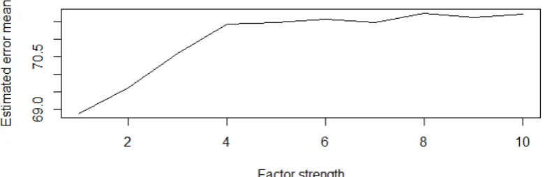
In Figure (2.1), I plot the average of F −

˜

Fr

over 1000 simulations vs. the value

of 1_/_γ. The value in the vertical axis (so called Estimated error mean) represents

how the estimated factors are dierent from the true factors. Inside the norm, F is simulated as described above and _F˜r _{is estimated by PCA as shown in Section 2.1.}

From this gure, it can be seen that the estimators are more precise when the factors are stronger, especially we observe a sudden change in estimation error when the strong factors just start to be weaker. In Figure (2.2) reports the standard deviation of

F − ˜

Fr

in 1000 simulations (so called Estimated standard deviation),

(45)

[image:45.595.88.479.192.319.2]

Figure 2.1: Estimated factor errors vs. pervasiveness (1 corresponds to strong factors)

Figure 2.2: Estimated factor errors standard deviation vs. pervasiveness (1 corre-sponds to strong factors)

[image:45.595.90.480.477.625.2]

(46)

2.5 Proofs of results

2.5.1 Proofs of Theorem 2.1

Since_F˜r_/√_T _{is the matrix whose columns are the orthonormal eigenvectors of}_{Y Y}0

by denition (the√T term is to make sure that ( ˜Fr0F˜r/T) =Ir), we can write:

1

TY Y

0_F_˜r _{= ˜}_Fr_V_˜

where_V˜ _{is the diagonal matrix whose diagonal consists of the} _r _{largest eigenvalues} ofY Y0/T. Clearly, the eigenvalues ofY Y0/T are the same as the eigenvalues ofΣ =˜

Y0Y /T, provided thatr <min(N, T). Therefore, as introduced in the preliminaries of section 2: _V˜ ₌_diag_(˜_v₁_{, ...,}_v_˜_r₎_.

We use a similar decomposition in Bai (2003): LetHr = ˜V−1F˜r0FΛ0Λ/T

˜

Fr−F Hr0 = 1

TY Y

0_F_˜r_V_˜−1₋ 1

TFΛ

0_Λ_F0_F_˜r_V_˜−1 =

Y Y0

T −

FΛ0ΛF0 T

˜

FrV˜−1

=

Y Y0

T −

FΛ0ΛF0 T

˜

FrD−_N1DNV˜−1

=

FΛ0U0

T +

UΛF0

T +

U U0 T

˜

FrD−_N1DNV˜−1

Notice that 1

T PT t=1 ˜

f_sr−Hrft

2

= _T1 ˜

Fr−F Hr0

2

F, so we can prove that

1 T ˜

Fr−F Hr0

2

F =

Op(_[_d N

r(N)]2 +

N2

T[dr(N)]2). In addition, notice that

˜

Fr−F Hr0 is aT×r matrix, so it only has r non-zero singular values, where r is a nite number. Therefore, we can use the operator norm in the subsequent proofs, which makes the notation easier.

For part (i) of theorem 2.1, we shall prove that 1

T

F˜

r₋_{F H}r0 2

=Op(_[_d N

(47)

N2

T[dr(N)]2)via Cauchy Schwartz inequality:

1

T

F˜

r₋_{F H}r0 2

≤ DNV˜

−1 2 ₁ T ( 1

TFΛ

0

U0F˜rD−_N1

2 + 1

TUΛF

0_F_˜r_D−1

N 2 + 1

TU U

0_F_˜r_D−1

N 2) .

From here, the (i) part of theorem 2.1 is proven by lemma 2.1, 2.2 and 2.3. The dominated term in these is

1

TU U

0_F_˜r_D−1

N

2

, which has orderOp(_[_d N

r(N)]2+

N2

T[dr(N)]2),

the remaining 2 terms in the big curly bracket has orderOp(

D_N−1

+_T1) =O_p(_d 1 r(N)+ 1

T), whereas

DN

˜

V−1

=Op(1).

For the (ii) part, rst we notice thatHrhas eigenvalues bounded from both 0 and

∞ by lemma 2.4, hence its inverse Gr exists. Similarly with the rst part, we will prove using the operator norm of the matrix_Λ˜r₋_Λ_Gk _{for easier notation. We now}

use the following decomposition:

˜

Λr=Y0F˜r/T

= ΛGrHrF0+U0F˜r/T

= ΛGrHrF0−F˜r0+ ˜Fr0F˜r/T +U0F˜r−F Hr0+F Hr0/T

= ΛGr+ ΛGr

HrF0−F˜r0

˜

Fr/T +U0

˜

Fr−F Hr0

(48)

2.5 Proofs of results Therefore, 1 N Λ˜

r₋_Λ_Gk 2

≤ 1

N T2 ΛG

k_Hk_F0₋ _˜

Fr0

˜ Fr 2 + 1

N T2 U

0_˜

Fr−F Hr0

2

+ 1

N T2 U

0_{F H}r0 2 ≤ 1 T H

k_F0₋_F_˜r0 2 ˜

Fr0F˜r T

Λ0Λ

N G k 2 +

U U0 N T 1 T ˜

Fr−F Hr0

2

+ 1

N T2 U0F

2 H r0 2

=Op

N

[dr(N)]2

+ N

2

T[dr(N)]2

by theorem 2.1, and the fact that Gk

= Op(1) if _T1

H

k_F0₋_F_˜r0 2

= op(1),

H

r0

=Op(1). Furthermore,

U U0

N T

is bounded above as U has nite entries and

the size ofU isN×T. For similar reason, _{N T}1 kU0Fk2 is bounded away from innity,

which establishes the nal result above.

2.5.2 Technical Lemmas

Lemma 2.1. Under assumption 1-5,DNV˜−1 has eigenvalues asymptotically bounded

away from both0and∞, where as introduced in the preliminaries: V˜ =diag(˜v1, ...,v˜r),

˜

v1 is the ith largest eigenvalues of Σ˜.

Proof. We have:

DNV˜−1 ≡

     

d1(N)

˜

v1 0

...

0 dr(N) ˜ vr      

It suces to prove that v˜i di(N) for every i ∈ (1, ..., r). First of all, we need to

state Weyl's Theorem: Let {ai}Ni=1 be the eigenvalues of A in descending order.

(49)

kA−Bk.

Ifµi(Λ0Λ)is theith largest eigenvalue ofΛ0Λ andΛΛ0. So by Weyl's Theorem, we

have:

v_i−µ_i(Λ0Λ) ≤

Σ−ΛΛ0

=kΣ_uk=O_p(1).

Therefore sinceµi(Λ0Λ)

Λ(i)

d_i(N) as in assumption 3(ii), v_i d_i(N). Now,

again by Weyl's Theorem:

vi−v˜i

di(N)

≤ Σ−Σ˜

/di(N) =Op(

N di(N)

r logN

T ).

The result Σ− ˜ Σ

can be found for example in Fan et al. (2011). Since by

assump-tion 4(ii) we have that N di(N)

q logN

T =o(1),vi di(N) impliesv˜i pdi(N).

Lemma 2.2. 1

T

1

TFΛ

0_U0_F_˜r_D−1

N

2

=Op(

D−_N1

)and _T1

1

TUΛF

0_F_˜r_D−1

N

2

=Op(

D−_N1

).

Proof. We have that:

1 T 1

TFΛ

0_U0_F_˜r_D−1

N 2 ≤ D−_N1

1 T D

−1/2

N Λ

0_U0 2 1

TF˜

r0 ˜ Fr 1 TF 0_F ≤ D−_N1

1 T T X t=1 D

−1/2

N Λ 0 ut 2

=Op(

D −1 N )

as by assumption 4 (iii) D

−1/2

N Λ 0_u t 2

= Op(1). Similarly, _T1

1

TUΛF

0_F_˜r_D−1

N 2 =

Op(

D_N−1

).

Lemma 2.3. 1

T

1

TU U

0_F_˜r_D−1

N

2

=Op

N

[dr(N)]2 +

N2

Weak factor model in large dimension

University of Warwick institutional repository: http://go.warwick.ac.uk/wrap

A Thesis Submitted for the Degree of PhD at the University of Warwick

http://go.warwick.ac.uk/wrap/69442

This thesis is made available online and is protected by original copyright.

Please scroll down to view the document itself.

Weak factor model in large dimension

by

Quang Phan

March 21, 2015

Thesis submitted in partial fulllment of the requirements for the

degree of

Doctor of Philosophy

Contents

List of Figures

List of Tables

Acknowledgment

Declarations

Abstract

1 Introduction

1.1 Literature review

1.2 Contributions of this thesis

2 Factor identication under the

weaker assumption

2.1 Factors identication techniques

2.2 Notations

2.3 Asymptotic results

2.4 Illustrated simulations

2.5 Proofs of results