warwick.ac.uk/lib-publications
A Thesis Submitted for the Degree of PhD at the University of Warwick
Permanent WRAP URL:
http://wrap.warwick.ac.uk/79564
Copyright and reuse:
This thesis is made available online and is protected by original copyright.
Please scroll down to view the document itself.
Please refer to the repository record for this item for information to help you to cite it.
Our policy information is available from the repository home page.
Theoretical Investigation of Solid State Cooling
Using Spin Models
by
Matthew Bates
Thesis
Submitted to the University of Warwick for the degree of
Doctor of Philosophy
Department of Physics
Contents
List of Tables iii
List of Figures iv
Acknowledgements vi
Declarations viii
Abstract ix
Chapter 1 Introduction 1
1.1 Introduction . . . 1
1.2 Caloric Materials and Caloric Effects . . . 3
1.3 Ferroelectrics . . . 3
1.4 Relaxor Ferroelectrics . . . 5
1.5 Polymers . . . 9
1.6 Antiferroelectrics . . . 10
1.7 Magnetocalorics . . . 11
1.8 Key Features From the Literature . . . 12
Chapter 2 Classical Physics of a Cooling Cycle 14 2.1 Cooling Cycles . . . 14
2.2 The Carnot Cycle . . . 14
2.3 Metrics of Performance . . . 17
2.4 The Maxwell Relations . . . 19
Chapter 3 The Statistical Mechanics of a Cooling Cycle 22 3.1 Introduction to Statistical Mechanics . . . 22
3.2 The Canonical Ensemble . . . 22
3.4 Hysteresis Cycles and Hysteresis Losses . . . 30
3.5 Mean Field Theories . . . 32
3.6 Variational Methods . . . 36
3.7 Caloric Effects . . . 39
3.8 The Einstein Model of Solids . . . 39
3.9 Isothermal Entropy Change . . . 41
3.10 Adiabatic Temperature Change . . . 42
3.11 Tuning a System to Tricritical Points . . . 43
Chapter 4 Modelling Materials 50 4.1 Disorder and Hysteresis . . . 50
4.2 Coupling Disordered Spins to a Thermal Lattice . . . 58
4.3 Modelling P(VDF-TrFE) . . . 60
4.4 Modelling Iron Rhodium . . . 62
Chapter 5 Binary Tree Graphs 82 5.1 Background Methodology . . . 82
5.2 Depth of the First Leaf . . . 85
5.3 Depth of the Second Leaf . . . 87
5.4 Solving the Depth of themth Leaf . . . 89
5.5 Leaf to Leaf Paths . . . 91
5.6 Further Investigations . . . 95
Chapter 6 Conclusions and Future Work 96
Appendix A Temperature Dependence of Maximum Applied Field
Strength in Hysteresis Loops 99
List of Tables
4.1 Values of peak height for C2 6= 0 with the peak height of C2 = 0
subtracted at both the AFM-FM and FM-PM transitions to 3 sig-nificant figures. This shows a much larger magnitude change for the normalised peak height at the AFM transition that at the FM-PM transition. . . 71 4.2 Percentage change peak height forC2 6= 0 compare to the peak height
ofC2 = 0 at both the AFM-FM and FM-PM transitions to 3
signifi-cant figures. This shows that the percentage change at each transition is approximately the same for the sameC2 value. . . 71
4.3 Temperature difference between the locations of the peak height for ∆Siso forC2 6= 0 when compared toC2 = 0 at both the AFM-FM and
List of Figures
1.1 A Hysteresis Loop . . . 5
1.2 Unit Cell of a Perovskite . . . 7
1.3 P(VDF-TrFE) . . . 10
2.1 Carnot Cycle . . . 15
2.2 Cooling Cycles . . . 16
2.3 Temperature-Entropy Diagrams . . . 17
3.1 Two Dimensional Lattice Orderings . . . 26
3.2 A Second Order Transition . . . 27
3.3 A First Order Transition . . . 28
3.4 A Two Dimensional Phase Diagram . . . 30
3.5 Hysteresis Losses . . . 32
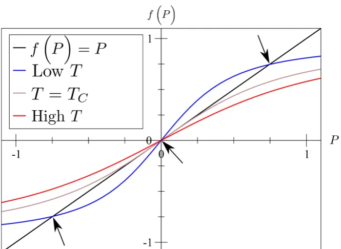
3.6 Graphically Determining The Polarisation . . . 35
3.7 Antiferroelectric System Configuration . . . 45
3.8 Antiferroelectric Polarisation and Order Parameters. . . 46
3.9 Antiferroelectric System Under a Small External Field . . . 47
3.10 Antiferroelectric System Under a Large External Field . . . 47
3.11 Finding the Tricritical Point . . . 49
3.12 Entropy Change Around the Tricritical Point . . . 49
4.1 Pure System Hysteresis . . . 52
4.2 Polarization Avalanches . . . 52
4.3 Disordered System Simulated Hysteresis . . . 54
4.4 Disordered System Experimental Hysteresis . . . 55
4.5 Simulated Hysteresis Loop for P(VDF-TrFE) . . . 55
4.6 Diagrams of the Ising, Isotropic- and Anisotropic-Heisenberg models 57 4.7 Simple ECE Analysis . . . 60
4.9 Prediction of ECE for P(VDF-TrFE) . . . 61
4.10 FeRh Unit Cell . . . 63
4.11 Single FeRh Free Energy . . . 67
4.12 Magnetisation and Order Parameters of FeRh . . . 69
4.13 Ordered FeRh Result . . . 70
4.14 Disordered FeRh Results . . . 71
4.15 FeRh ∆Siso . . . 72
4.16 FeRh ∆Tadi . . . 72
4.17 FeRh ∆Siso for Varying x . . . 73
4.18 FeRh ∆Tadi for Varyingx . . . 74
4.19 FeRh ∆Siso for Varying Applied Field . . . 75
4.20 FeRh ∆Tadi for Varying Applied Field . . . 76
4.21 Experimental results, FeRh ∆Siso for Varying Applied Field . . . 76
4.22 Experimental Results, FeRh ∆Tadi for Varying Applied Field . . . . 77
4.23 FeRh magnetocaloric strength measurements . . . 78
4.24 The simulated refrigerant capacity of FeRh . . . 79
4.25 The Full Width at Half Maximum of ∆Tadi and ∆Siso . . . 80
4.26 Peak Values of ∆Siso in FeRh . . . 81
4.27 Peak Values of ∆Tadi in FeRh . . . 81
5.1 A Binary Tree Diagram . . . 83
5.2 Counting First Leaf Depth . . . 83
5.3 Tree Graph Decomposition . . . 84
5.4 Connecting Nearest Neighbour Leaves in Sub-Trees . . . 86
5.5 Counting Second Leaf Depth . . . 88
Acknowledgements
There are no words to truly describe the numerous ways in which so many people have supported me and shaped my life, this project and this thesis during my time at Warwick in the last four years. Indeed I may, on reflection, decide that it is necessary to thank everyone that I have met (whether I have been able to get to know them or not) during my entire life, as they have all led me to this point.
You will forgive me, then, if these acknowledgements sound a little like an Oscar acceptance speech, I find it very difficult to not get emotional and poetic under circumstances such as these, the closing of a chapter of my life.
An attempt shall be made to thank only those whose influence has directly led to benefits to this project, to avoid putting myself in some situation where I am left thanking the whole world.
With the flowery introduction out of the way I would first and foremost like to thank my supervisor, Professor Julie Staunton, for all of her help during the project and getting the thesis into the shape it is. I would also like to thank my family: Mum, Andy and Dad, you have all helped me more than you may ever know, giving me inspiration and motivation for not just this project but all aspects of my life. After this it becomes a challenge to thank people in some order without giving offence or risking forgetting someone, so please bear with me as I collect people together as indistinguishable particles and thank them in alphabetical order.
might have gone stir crazy) and your patience with me and my messy ways I thank you, it has been a privilege to live with all of you and to have learned from you all. MathsPhys society, this set (not group!) encompasses a great many people to whom I am thankful for different things, but the unifying connection was (and somehow, remains to be) the MathsPhys society and for that I will always be thankful, I hope we see each other again soon. PS0.01 (and assorted hangers on), my thanks for the various conversations (including, but not limited to, those that were productive, entertaining and #Deep) and support that you all provided me whether I was brave enough to ask for it or not. The University of Warwick Mixed Hockey Club (and Berkswell), you reminded me that life wasn’t all about work and I had to get on it (for once) from time to time, whenever I was having a bad time, being able to vent steam at some hockey balls and run like a maniac around the pitch helped me get some perspective back, it has been a privilege to know you all.
Having said that I would not single anyone out, I find it necessary to thank (in alphabetical order) Drs. Bennett, McDonald and Refaat for their advice and support in getting this thesis written.
Declarations
This thesis is submitted to the University of Warwick in support of my application for the degree of Doctor of Philosophy. It has been composed by myself and has not been submitted in any previous application for any degree.
The work presented (including data generated and data analysis) was carried out by the author except in the cases outlined below:
Figure 3.4 was reproduced from reference [69]. Figure 4.4 was reproduced from reference [78]. Figure 4.8 was reproduced from reference [31]. Figure 4.21 was reproduced from reference [61]. Figure 4.22 was reproduced from reference [85].
Abstract
A mean field spin model coupled to a thermal model of a solid is used as a de-scription of the electrocaloric effect in relaxor ferroelectrics at both first and second order transitions. This theoretical model is also used in efforts to find the tricrit-ical point of transitions to maximise the adiabatic temperature change due to the electrocaloric effect while minimising the hysteresis losses in a cooling cycle. The electrocaloric effect is the adiabatic temperature change exhibited by a material un-der the sequential application then removal of electric fields. Relaxor ferroelectrics are materials with two interaction scales, local interactions in polarised nano regions (PNRs) and longer range interactions between PNRs. Electric dipoles are modelled as spins and their alignment due to an external field is used to examine polarisation-electric field loops. The results are compared to experimental data to determine values of parameters that may be used in simulations to model the electrocaloric effect. I reproduced simulations of the electrocaloric effect in the ferroelectric ma-terial lead zinc niobate-lead titanate [Pb(Zn1/3Nb2/3)O3-PbTiO3] by coupling the
room temperature has promise for replacing conventional refrigerants.
Due to the simplicity of this coupled model and the physical similarities between the electrocaloric effect and the magnetocaloric effect (an analogous effect observed in certain magnetic materials where an adiabatic temperature change is seen under the application and removal of a magnetic field) an investigation is also carried out on the magnetocaloric material iron rhodium (FeRh). In simulations I varied global and local stoichiometry to affect the ordering of spins and thus the entropy and strength of the magnetocaloric effect. I compared the results of our simulations with experiment and examine the variation in peak isothermal entropy change and adiabatic temperature change under variation in stoichiometry as well as the effects on the full width at half maximum. The results show that a simple model can give a qualitative representation of the effect.
Chapter 1
Introduction
1.1
Introduction
Since 1834 [1], the developed world has enjoyed the benefits of the vapour com-pression refrigeration cycle and the fantastic cooling power that it brings. In the summer in the United States of America, up to fifty percent of energy consumption is used for some form of cooling [2].
The best vapour compression refrigerators designed today reach a maximum of fifty-five percent of the ideal Carnot efficiency [3] which is likely close to the limits of what will be possible in this mature and well studied field. Many refrigerants cur-rently used in a vapour compression cycle come from the Hydrofluorocarbon (HFC) family [4]. HFCs are used as a substitute for earlier ozone depleting refrigerants and represent 89 percent of US fluorinated gas emissions [5]. As fluorinated gases have a large CO2 equivalent [6] this means that HFCs may account for up to 45 percent
of the world’s CO2-equivalent emissions by 2050 [4]. If an alternative method of
refrigeration could be found that is less energy intensive then it would be cheaper for the end user and less polluting for the environment.
This means that a large step could be taken in tackling the issue of global warming if a more energy efficient refrigeration system using less polluting materi-als should be developed. Solid state refrigeration using various caloric effects could provide this solution. A caloric effect is where the application and subsequent re-moval of some external force causes an isothermal entropy change which leads to an adiabatic temperature change [7].
per-cent [8]. The electrocaloric effect, achieved with the application of an electric field, has the chance to be more readily applicable than the magnetocaloric effect due to the relative ease of generating large electric fields in comparison with magnetic fields. The substitution of rare earth elements in a refrigerant can enhance the magnetocaloric effect [9], however due to geopolitical reasons the supply of rare earths is expensive and unreliable. Giant electrocaloric effects have been found with materials that are widely available [10] and with a more detailed understanding of the mechanisms behind the electrocaloric effect it may be possible to optimise an electrocaloric refrigerant to produce an effect as strong or even stronger than that of the magnetocaloric effect.
The thesis will be structured as follows. The rest of this chapter will present a brief overview of the field of electro and magnetocalorics as relevant to the work presented in this thesis, this will set the scene for the work undertaken but is, by no means, an exhaustive review of the literature.
I will use chapter 2 to discuss the thermodynamics of a cooling cycle intro-ducing the mathematics and methodology as well as the efficiencies and metrics that will be useful in describing the electrocaloric effect.
I shall then introduce statistical mechanics in chapter 3 to provide a general description that can be applied to a refrigerant, including the description of the phase transitions that it must pass through to maximise the strength of the electrocaloric effect and addressing potential sources of loss during a cooling cycle.
In chapter 4 I present a simple model of spins (to represent the electric dipoles of a refrigerant) coupled to a phonon lattice that will enable us to describe the isothermal entropy changes and adiabatic temperature changes that the system undergoes during a cooling cycle. Novel work is carried out to investigate the tri-critical point of antiferroelectric to ferroelectric phase transitions using our model. I will then collate the ideas introduced in the previous chapters and use them to re-produce simple models from the literature. This re-produces an understanding of how the basic ingredients examined earlier in the thesis lead to a successful model of solid state cooling. This chapter will demonstrate the novel work done on applying our model of electrocalorics to the analogous field of magnetocalorics to examine the isothermal entropy change and adiabatic temperature change in iron rhodium and how the peak and widths of these responses are affected by the disorder in the material.
binary tree graphs of a given size and the number of vertices on a path between any two leaves of the tree.
Finally chapter 6 summarises the work in the thesis and provides a discussion for how work may proceed in this area.
1.2
Caloric Materials and Caloric Effects
The field of electrocalorics is relatively young in comparison with both the field of magnetocalorics and that of the well researched traditional vapour compression cycle, yet there is already much written on the subject. In the next few sections we shall review some of the topics relevant to this thesis, namely the properties of ferroelectrics and relaxor ferroelectrics, thin film polymer relaxor ferroelectrics and anti ferroelectrics and their suitability in electrocaloric applications.
1.3
Ferroelectrics
Ferroelectricity was first reported in 1920 by Valasek [11] and was so named due to the similarity of the permanent electric dipole to the permanent magnetic moment observed in ferromagnetic materials. Shortly after the discovery of ferroelectricity came the realisation of the electrocaloric effect in Rochelle salt in 1930 [12] which can be seen as analogous to the magnetocaloric effect found in 1881 [13]. However, due to the weakness of the effect in traditional ferroelectrics, it was another twenty five years before the electrocaloric effect was revisited with the possibility of creating a practical cooling cycle [3].
Just as ferromagnetic materials at sufficiently low temperatures have an in-trinsic alignment of magnetic spins without the application of any external magnetic field, ferroelectric materials have a spontaneous net alignment of electric dipoles even without the presence of an external electric field [14]. Above the Curie temperature (TC) of a ferroelectric/magnetic (FE/FM) material exists the
paraelectric/param-agnetic (PE/PM) phase where the electric/mparaelectric/param-agnetic spins are unaligned and there is no net polarisation/magnetisation. Cooling below TC the spins begin to align in
the FE/FM phase.
In ferroelectrics this transition is often associated with a structural transition, such as a small displacement off centre of the titanium ion in lead titanate (PbTiO3)
when the material changes from a cubic to tetragonal structure on passing below
TC [15], this asymmetry in the unit cell causes a dipole to form along the direction
Ferroelectrics have competing short range and long range order. Short range order causes the formation of domains within the ferroelectric where the electric dipoles of individual unit cells are all aligned in the same direction. The long range order within a ferroelectric is the alignment of the domains which are less strongly linked than individual dipoles. The interfaces between domains of differing alignment are called domain walls, these have an associated energy which is the difference between the ground state energy (found in the situation with the wall) and the energy of the system with all dipoles aligned. As an external field is applied the domain walls will move as dipoles align with the external field, domains aligned with the field will grow in size while those not aligned will shrink. Thus the discussion of the free energy and entropy of a ferroelectric ought to use a macroscopic model to consider the details of the domains and domain wall motion rather than individual dipoles.
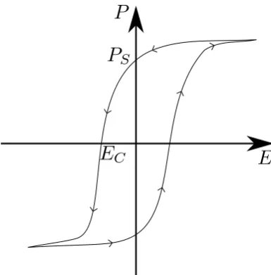
Ferroelectric materials are, by definition, associated with polarisation hys-teresis under the application and removal of an electric field. Hyshys-teresis is the effect observed when there is a delay in response from a system with respect to an external stimulus. For example a paraelectric system will show no hysteresis, freely aligning itself with an externally applied field instantly, whereas a ferroelectric system has an intrinsic polarisation before the application of the external field. Should the field point anti-parallel to this polarisation, the polarisation will not immediately align with the field but there will be a delay until the field is sufficiently large before the polarisation aligns with field as shown in figure (1.1) [14].
Energy is put into the material in destroying, creating and moving the domain walls to allow the domains to fully align with the field. This is energy that is not used in creating an isothermal entropy change (∆Siso) and thus is energy input that,
under a cooling cycle, would be wasted (see section (3.4) for more details).
Figure 1.1: A hysteresis loop showing polarization against applied electric field oriented in the same axis. PS is the value of polarisation that
re-mains when the field is removed, called the remnant polarisation. EC is the
coercive field - the field strength required to reduce the polarisation to zero.
remnant polarisation of the material, this energy is lost every cycle and so reduces the efficiency of the system - this occurs for magnetic systems as well [17]. Large hysteresis is associated with the large entropy change of a first order transition (see section (3.3)) while second order transitions are associated with significantly reduced hysteresis losses [18]. It is possible to determine polarisation hysteresis loss from polarisation hysteresis loops [19].
It has been discovered more recently that not only can the direct (or positive) electrocaloric effect occur where the application of an external field leads to an initial increase of temperature of the material (the removal of the field then leads to a decrease of temperature which leads to the cooling cycle), there is also an inverse (negative) electrocaloric effect [20] where the application of the field leads to a decrease of temperature [21] - it is even possible to see both signs of the effect in one material at different phase transitions, e.g. antiferroelectric-ferroelectric and ferroelectric-paraelectric [22].
1.4
Relaxor Ferroelectrics
Experimentally there have been found to be two temperatures of interest in relaxors [23] where peaks have been observed in both the strength of the elec-trocaloric effect [24] and the electric permittivity of the sample [25]. This leads to a description of the formation and alignment of polarised regions on the scale of nanometres (Polar Nano Regions or PNRs) [26]. At very high temperatures, relaxors experience a paraelectric (PE) phase (which is the same as as a PE phase in a tra-ditional ferroelectric), on cooling they pass through a so called ergodic relaxor (ER) phase [27] in which the PNRs form, these are local clusters of alignment embedded in the material which itself has a random orientation of dipoles. This alignment occurs as the material is cooled from the PE phase to below the Burns tempera-ture, TB. Even further below this there is the freezing temperature (Tf) at which
the PNRs become frozen in orientation and the relaxor becomes non-ergodic [28]. For temperatures Tf < T < TB, the PNRs are free to independently explore the
phase space and the vector of the electric dipole may point in any direction, hence the term ER. Below Tf, should an external field be applied then the PNRs would
align and the material would behave as a ferroelectric. Heating an aligned relaxor aboveTf again will return it to the ER phase. Phase transitions in relaxors occur
across a broader range of temperature than those found in traditional ferroelectrics which are localised to one temperature [21]. This is due to the variation in size and relative strength of the PNRs, with this variation they form and align across a range of temperatures (centred aroundTB andTf respectively) leading to a diffuse
transition not observed in pure ferroelectrics. There have been models describing the size and distribution of PNRs with statistical mechanics ([29], [30], [31]) and this school of thought will influence this thesis.
A key structural difference between ferroelectrics and relaxors is the lack of long range structural order in relaxors [32] at high temperatures, the breaking of the regular, ordered system into distinct PNRs [33] removes the order found in aligned ferroelectrics. The relaxors, however, develop long range coherence below Tf [15]
and thus we may assume long range order in the system [34] even though it may not, at first glance, be expected. Note also that the transition into the FE phase in a ferroelectric is driven by a structural transition, while relaxors can become polarised in an external field at TB and a remnant polarisation will be kept only below TF
and neither temperature is necessarily a structural transition.
compared with regular ferroelectrics [37] is due to the expansion and contraction of the PNRs under external fields [38] which is not present in ordinary ferroelectrics. This strain in the material can induce a secondary electrocaloric effect which is often neglected in theoretical treatments even though it may contribute significantly to the total isothermal entropy change [3].
Traditional relaxors are a subset of the inorganic ferroelectric crystals with a perovskite structure i.e.ABX3 where A andB are cations and X is an anion,
usu-ally oxygen, which binds to both - for example PbTiO3 [28] as shown in figure (1.2).
These crystals were originally lead based [3] although more recently lead free com-pounds have been created which still have an appreciable electrocaloric effect [39]. In order to increase the strength of the effect, relaxors often have substitution of elements on the B site to introduce compositional disorder to the system and this can be controlled by the way the material is formed with quick annealing from high temperatures not allowing the system to reach a (complex) ordered ground state, but instead resting in a metastable state [28].
Figure 1.2: PbZnO3 −PbTi3, an example of the unit cell of a cubic
per-ovskite. A system of purely PbZnO3or PbTiO3would be a regular
ferroelec-tric which goes through a structural phase transition atTC from tetragonal
(with a displacive central ion leading to an electric dipole) to cubic (regu-lar with no displacive ion, thus no spontaneous po(regu-larisation). The disorder caused by the possible substitution of a zinc ion in place of a titanium ion or vice versa causes the change to a relaxor.
Such a crystal relaxor system (Pb(Zn1/3Nb2/3)O3-PbTiO3 also called
the strength of the externally applied electric field. They found that the effect was weak far below the Curie temperature (TC) of the material, rapidly increased and
peaked atTC and then slowly decreased beyondTC (see figure (4.8) in section (4.2)).
They created a simple mean field model of Ising spins (here modelling dipoles of the mobile titanium ions in the unit cells of a PNR) coupled to an Einstein lattice to simulate the behaviour of the dipoles and the connection with phonon activity in their crystals. Disorder in this material is modelled from the variety in the transition temperatures of the PNRs. The results (see figure (4.7) in section (4.2)) hold well below TC, but predict that the electrocaloric effect will drop away rapidly above
TC. This suggests that above TC the interactions between the electric dipoles of
the PNRs is not the only contribution to the electrocaloric effect. The literature suggests that while the interactions between PNRs may cease to overcome thermal agitation above TC, the PNRs continue to exist and so may be aligned under an
external field until their destruction at the Burns temperature and this allows for the continued existence of the electrocaloric effect [40].
As the strength of the effect is partly related to the coupling of the relaxor to the external field, the limitations of the electrocaloric effect have been the maximum strength of field that may be applied, restricted by the electric breakdown strength of the specimens [41] beyond which point the relaxor becomes conductive and a cooling cycle cannot be created. Moving from a bulk crystal to a thin film material allows larger fields to be applied leading to a greater adiabatic temperature change [42]. There is a general inverse relationship between the breakdown field strength and film thickness [43] which is due to the different mechanisms that lead to breakdown in thin films and bulk materials. In bulk materials the electric breakdown strength is proportional to the square root of the Young’s modulus and micro cracks in the material can lower the Young’s modulus, thus weakening the dielectric breakdown strength [44]. In thin films the Young’s modulus is significantly greater and the dominant contribution turns out to be an ionisation avalanche [3] where one part of the film becoming ionised induces ionisation in its neighbours and this spreads through the material.
are reorientable and count towards the random bonds whereas the random chemi-cal clusters are static in the material and so provide a permanent, on site random field, the disorder (randomness) of both comes from the great variation in size and location of PNRs and chemical clusters within a relaxor. This model is based on the experience of the authors in the field of spin glasses and, indeed, is solved using the replica method as one may do with spin glasses.
1.5
Polymers
The advantage of thin films over bulk materials is their higher dielectric break-down strengths meaning they can be exposed to larger fields and produce a larger adiabatic temperature change (∆Tadi), ferroelectric polymers may have even larger
dielectric breakdown strengths leading to the opportunity for greater ∆Tadi [3].
Present research is concentrated around poly(vinylidene fluoride-trifluoroethylene) or P(VDF-TrFE) [21] possibly with the addition of chlorofluoroethylene to make the terpolymer P(VDF-TrFE-CFE) [26]. Such polymers may be electron irradi-ated to break up the large polarisation domains and form polar nano-regions (the spins of our model), thus creating a relaxor [45]. Polymers can also exhibit a large electrostrictive response to an applied external field (due to the flexibility of the PNRs and the surrounding medium) [37] increasing the strength of the secondary electrocaloric effect when compared with inorganic relaxors.
The chemical chain of P(VDF-TrFE) is shown in figure (1.3), the ferroelec-tric properties of the polymer chain come from the large variation in electronega-tivity of the constituent elements [46]. Electronegaelectronega-tivity is a measure of how strong the attraction is between an atom and a pair of covalent bonding electrons, with equal electronegativity the electrons will sit equidistant between two atoms, however should one atom have a larger electronegativity then it will attract the electrons to it and this displacement of the electrons will induce an electric dipole [47]. Fluorine has an electronegativity of 4.0 on the Pauling [48] scale while carbon and hydrogen have values of 2.6 and 2.2 respectively (for reference the least electronegative ma-terials are caesium and francium with a value of 0.7). A rule of thumb [47] is that for an electronegativity difference of around 2 the interactions could be considered ionic, so we can see that the fluorine atoms will exert an almost ionic character on the system, leading to strong electric dipoles.
Figure 1.3: The monomers of the P(VDF-TrFE) copolymer
physically realistic model of relaxor polymers is infeasible, but perhaps the model created for crystal relaxors would be a good starting point.
That was the thinking of Pirc et al. [26] who adapted their SRBRF model ([36], see the previous section) for a crystal relaxor and used it to model a polymer, they take the various grains in the polymer to be the sources of PNRs and produced the same Hamiltonian as before with the same Gaussian distribution of interaction strengths and random fields. The main differences to their previous work is the argument that there are far fewer random chemical clusters in the polymer than in the inorganic crystal and thus the effect of the random fields is weaker.
1.6
Antiferroelectrics
As a ∆Siso leads to a large ∆Tadi, finding materials which display such an entropy
change is important. Such changes need not only occur at the ferroelectric to para-electric transition but also at an antiferropara-electric to ferropara-electric transition and these have been found in inorganic relaxors [24], [42] (note that both of these references show positive electrocaloric effect at both transitions). Should the applied external field induce a phase transition, then the difference between the order parameters of the antiferroelectric and ferroelectric phases could cause a large ∆Siso.
The coexistence of competing phases is reminiscent of the work of Imry and Wortis [50] where they suggest that, should different regions of a material have different transition temperatures (note that the transition does not need to be an-tiferroelectric to ferroelectric, it could be any other transition as long as there is a change of phase) one would expect to find a diffuse transition peak rather than a sharp transition at the transition temperature, TT; relaxors have a diffuse phase
would change phase at the TT it would have were it a bulk sample not in contact
with any other region. This, however, is not a full view of the picture as when one region changes phase it would create a phase interface between it and its neigh-bours, such an interface would have a free energy cost associated with it, should this cost be greater than the free energy gained by the region changing phase it would be energetically unfavourable for the change of phase to occur. This implies that inhomogeneity within the material can have an effect on a phase transition and thus on the ∆Siso and ∆Tadi that would be produced, it would be of interest
to observe this effect in both inorganic relaxors and the relaxor polymers to see the difference between the two and how changing the compositional disorder would affect the electrocaloric effect in each. Their model predicts that some fraction of regions will be able to exist in their energetically favourable phase within a bulk in a different phase this would lead to, at least, partial rounding of a first order phase transition as there would be different regions transitioning at different times, the model is unable to predict whether complete rounding (i.e. complete removal of the first order character of the transition) would occur or not.
Peng et al. examined antiferroelectric relaxors [24]. They explicitly observed a strong ∆Siso and ∆Tadi at the antiferroelectric-ferroelectric transition but also
the two temperature scales of a relaxor at the ferroelectric-paraelectric transition where many experiments reveal a single peak at the TC of the material, there is
in fact a clear double peak. Of these two peaks, the higher temperature one is associated withTB (i.e. where the PNRs begin to form, the ergodic relaxor phase)
and the lower with Tf (where they align and freeze). They point out that such a
double peak structure has been seen in relaxor ferroelectrics [23] in addition to their antiferroelectrics, thus suggesting that the double peak is not an artefact related to the antiferroelectric nature of their material lead barium zirconate but is related to the formation and freezing of PNRs.
1.7
Magnetocalorics
The magnetocaloric effect (the magnetic equivalent of the electrocaloric effect) was first observed in 1881 by Emil Warburg [13], far before the electrocaloric effect. Initially harnessed to cool below liquid helium temperatures (using materials such as cerium magnesium nitrate) it was more thoroughly investigated than the elec-trocaloric effect as the first magnetocaloric materials displayed a larger temperature change than the first electrocaloric materials under similar field strengths.
Gd5(Si2Ge2) at room temperature in 1997 [52], this suggested that magnetocalorics
could be applied to room temperature refrigeration.
One magnetocaloric of particular interest in this project is iron rhodium (FeRh). FeRh forms a structure where there are unit cells with one atom type on the corners and the other atom type in the centre. However, at non-zero temperatures there is a non-zero probability of finding an Fe atom having displaced an Rh atom from the Rh lattice or vice versa (at least one or two percent of the sites may experience this after typical annealing processes [53], the higher the temperature the greater this probability). Thus if the system is quenched from a high temperature it may relax into a state with large deviation in local stoichiometry (the ratio of the constituent elements) from a global 50-50 mix.
Deviation from stoichiometry is an important consideration for FeRh as it is a magnetic material that is very sensitive to composition, even a 2% variation in iron concentration can completely remove a ferromagnetic to antiferromagnetic phase transition that exists when the material contains equal proportions of iron and rhodium [54]. The temperature of this transition can be readily changed by varying the way the sample is treated (e.g. via electron irradiation) [55].
Such sensitivity to composition makes FeRh an interesting material to study to examine the effects of local structural disorder. Such disorder is well suited to being modelled by the treatment of Vives et al. [16] mentioned earlier and as such makes a natural continuation of the investigation set up with the model that shall be produced in this project.
1.8
Key Features From the Literature
We have seen in this review of the literature that even inorganic, ferroelectric crystals are complex systems but that the key contribution to a model of the electrocaloric effect comes from the interactions between electric dipoles (vectors linked to particu-lar locations in the material - much like vector spins on a lattice) and the interaction with underlying structure in the material that compensates for any induced decrease in dipolar entropy. We also know that polymers are significantly more complicated materials to model, yet due to their high electric breakdown strength can exhibit a larger ∆Siso than bulk or thin film crystals. It is also clear that the large ∆Siso
associated with an antiferroelectric to ferroelectric transition can lead to a large ∆Tadi.
field is dominated by P(VDF-TrFE) which contains fluorine. If research can find relaxors without these environmentally damaging materials which also have a large ∆Tadi then there is strong justification for using the electrocaloric effect over
con-ventional refrigerants (such as the environmentally harmful HFCs) or the magne-tocaloric effect (which currently relies on rare-earth elements [21] and larger fields than the electrocaloric effect [3]).
Two key targets in research then are to create a general (not relaxor specific) model that, at the very least, produces qualitative agreement with experiment and has the predictive power to simulate parameters of different elements and suggest what the effect of the addition or removal of certain elements to a mix may be and how it compares to current relaxors. The other target would be an understanding of the mechanism behind the electrocaloric effect in the paraeletric phase, the models predict that this cannot be simply due to dipolar interactions.
Chapter 2
Classical Physics of a Cooling
Cycle
2.1
Cooling Cycles
It is important to be able to have an understanding of the phenomenology behind the cooling cycle we wish to employ and to have an estimate of the strength of the effect. This chapter will be concerned with producing a simple, general description of cooling cycles - reversible processes where due to external work done on a refrig-erant and heat exchange with the environment, the temperature of the refrigrefrig-erant is lowered such that it may be used to cool a volume. We shall examine these cycles using classical thermodynamics before describing important quantities to measure for comparison between refrigerants and then telling of the phenomenology of a general caloric cycle.
2.2
The Carnot Cycle
The maximum efficiency that an ideal cooling cycle can achieve is called the Carnot limit and is reached by the Carnot Cycle [56]. In the general case a cycle runs as follows: reversible, adiabatic work (also called isoentropic work as entropy remains constant because there is no heat or matter transfer) is done on the refrigerant to lower the temperature from a high value,T1 to a lower one,T2. In the second stage
heat is transferred to the system from a cold reservoir (the system is at a constant temperature, i.e. this process happens isothermally), then more isoentropic work is done on the refrigerant to increase its temperature back to T1 before the cycle is
system to the state in which it began. This process manipulates state variablesV1
and V2 which are pairs of thermodynamic parameters such as pressure and volume
[image:27.595.220.419.167.364.2]or entropy and temperature.
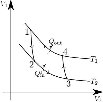
Figure 2.1: A Carnot cycle on state variables V1 and V2. Going from 1 to
2 is an isoentropic lowering of V1. Moving from 2 to 3 heat is transferred
isothermally (at constant temperature T2) from the substance to be cooled
to the refrigerant to increaseV2. From 3 to 4 isoentropic work increases V1,
then heat is transferred (at constant temperatureT1) from the refrigerant to
the environment between 4 and 1 to return it to its original state. Adapted from [57]
In figure (2.1), the area under the cycle is the amount of heat exchanged between the refrigerant and the object it is cooling, the area inside the cycle is the amount of work done by the surroundings. The efficiency of the cooling cycle (the Carnot efficiency) is the ratio of the work done over the sum of the heat exchanged and the work done, i.e.:
Efficiency = T1−T2
T1
= 1−T2
T1
(2.1) For a vapour compression system the first step is an isoentropic expansion of the vapour refrigerant lowering the pressure (one state variable, c.f. V1 in
fig-ure (2.1)) and, as a side effect, its temperatfig-ure. Heat applied to the refrigerant isothermally increases the volume (c.f. V2 in figure (2.1)) of the vapour at a
shown in the left hand side of figure (2.2).
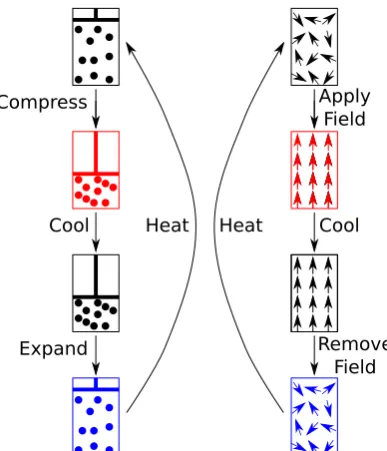
Compress
Cool
Expand
Heat
Apply Field
Cool
[image:28.595.223.417.130.356.2]Remove Field Heat
Figure 2.2: Vapour compression (on the left hand side) and electrocaloric (on the right hand side) cooling cycles for comparison where, in the first step, work is done to the refrigerant (compression in the case of vapour compression and application of an external field for electrocaloric), then heat is transferred away from the system. In the next step work is done in the opposite manner to before (expansion of the fluid or removal of the field), in the final step the refrigerant absorbs heat from the load to be cooled and the cycle is repeated.
T
S
Zero Field Applied Field
(a) The total entropy of a system with and without an applied field across a range of temperatures. The box is the region in figure (2.3b)
T
S
Zero Field Applied Field
[image:29.595.328.497.107.226.2](b) A magnified view of the isother-mal entropy and adiabatic tempera-ture changes around a phase transition
Figure 2.3: Comparing the total entropy (lattice and dipolar) under an applied field and under zero field to see the ∆Siso and ∆Tadi. A cooling
cycle happens in the following way: the refrigerant is at rest at A with temperatureT1 and entropySA. An external field is applied, increasing the
temperature to TB at constant entropy. As the refrigerant equilibrates its
temperature with the environment by releasing heat it moves fromB toC
returning to T1, effectively having undergone ∆Siso reducing the entropy
from SA to SC. As the external field is removed, there is an adiabatic
temperature change fromT1 toT2 which is the cooling observed during the
caloric effect. Heat is then absorbed from the load to be cooled to return the refrigerant to SA and TA. The largest entropy change occurs at the
phase transition as there is a structural change at this temperature which causes a large change in polarisation which in turn causes a large entropy change.
2.3
Metrics of Performance
When comparing potential refrigerants it is important to have well defined metrics to ensure that the reader is clear about the claims made by an author and that different refrigerants may be directly compared and contrasted. One refrigerant may have a large adiabatic temperature change (∆Tadi) with a very narrow peak
while another may have a moderate cooling across a wide temperature range, both may require a large external field to produce their cooling relative to the small field required by a third refrigerant. The metrics of performance discussed in this section will allow us to examine the benefits of potential refrigerants.
entropy changes atT1 and T2 must be equivalent and so, on a temperature-entropy
graph (if, for example, temperature and entropy were the state variablesV1 and V2
of figure (2.1)), the work done on the refrigerant is the area inside the cycle and is equal to ∆Tadi∆Siso, the refrigerant capacity. This means that the refrigerant
capacity can compare the relative cooling power (RCP) of an idealised system. Some groups [59], [17] report a similar comparison measuring the value of the RCP whereRCP =SIsoδTFWHMSIso measures the combination of the peak value
of the isothermal entropy change and width of the entropy at half the of the peak value (the subscript FWHM being short for Full Width at Half Maximum). This allows reviewers to discriminate against sharp peaks in ∆Siso [60]. Reporting the
peak ∆Siso may make it seem like a material has strong cooling power, but if this
peak is highly localised then the RCP would be low, showing that the refrigerant would make for a poor practical device when compared to another refrigerant with a more distributed generally high ∆Siso and a higher RCP.
The relation ∆Tadi
∆E (also called the electrocaloric strength, c.f. the
magne-tocaloric strength for magnemagne-tocalorics [61]), gives a measure of the temperature change when compared to the change in strength of the external field, ∆E. While a large ∆Tadiis a clear figure of merit to a cooling cycle, if these are achieved only at
the expense of a large applied field then the refrigerant needs a larger energy input than a refrigerant which possibly leads to a smaller ∆Tadi but does not require as
large a field. Results of ∆Tadi
∆E remove any dependence on experimental variables [3]
and report a measure of the intrinsic properties of an electrocaloric material. This figure should, however, be be treated with caution when considering practical cool-ing cycles as a refrigerant with large ∆Tadi
∆E but a small electric breakdown strength
(see section (1.5)) would mean that it is not possible to take full advantage of this large intrinsic effect to produce a powerful cooling cycle.
Another important number for consideration in practical cooling cycles is the coefficient of performance (COP) [21], a value equal to the cooling power over the input power. This represents the efficiency of a system in practice, including all losses to a hysteresis cycle (section (3.4)), Joule heating in the system from leakage currents, etc. The importance of this measurement is that, combined with the Carnot efficiency (see section (2.2)) we get a total measure of the possible cooling power of the system, the headline (technical) efficiency.
loses as little energy as possible from hysteresis or leakage currents (so, those closest to their Carnot efficiency) would be deemed the best refrigerants.
With a combination of the COP and ∆∆TE, we can compare and contrast differ-ent refrigerants to observe what qualities and properties distinguish refrigerants that have high COP and ∆∆ET, leading to an informed decision about new refrigerants to trial and how it may be possible to improve the strength of the electrocaloric effect in materials with high electric breakdown strength but weaker COP and∆∆TE. For exam-ple, a 55-45 mix of the polymer P(VDF-TrFE) has a similar ∆∆TE to PbSc0.5Ta0.5O3
(0.006 - 0.008 K cm kV−1, respectively), but due to the high dielectric strength of the polymer a larger ∆T can be obtained (12.6 K compared to 6.2 K), thus an examination of the COP would be of interest to determine whether the extra en-ergy input to create the larger ∆T is justified. Similarly PbZr0.95Ti0.05O3 has an
equivalent ∆T to P(VDF-TrFE) (12 - 12.6 K, respectively), but nearly three times as large a ∆∆ET (0.015 - 0.006 K cm kV−1). An investigation into the COP of both would determine whether this advantage is sustained in a repeated cycle. It should be noted that the different Curie temperatures of these materials (495 K, 353 K and 341 K for PbZr0.95Ti0.05O3, P(VDF-TrFE) and PbSc0.5Ta0.5O3 respectively) offers
an alternative reason why one material might be preferred to another, in this case. By comparing headline efficiencies we can directly compare the total cooling power of refrigerants. Simulations suggest that cooling systems based on materials with a large electrocaloric effect can have higher COPs (> 60% of Carnot effi-ciency [24]) than conventional vapour compression refrigerants [3], suggesting that cooling systems based on the electrocaloric effect can, indeed, produce more energy efficient refrigeration.
2.4
The Maxwell Relations
As described in section (2.2) a caloric cooling cycle comes about due to the appli-cation of an external force, in the case of the electrocaloric effect it is an external electric field acting on the electric dipoles of the system that leads to an isothermal entropy change (∆Siso). The field encourages increased polarisation (alignment of the electric dipoles) in the material thus decreasing their entropy.
To obtain a description of these processes we specify the free energy of the system:
F = (U −TS)−E~ ·P~ (2.2) whereU is the internal energy of the system,T is the temperature, Sis the entropy,
~
E is an externally applied field andP~ is the value of the polarization of the system. From equation (2.2) taking the polarisation and external field to be aligned in the same direction direction (therefore treating them as scalars) and by assuming that all quantities are continuous across the phase transition (i.e. that the phase transition is second order rather than first order), it is possible to derive the following Maxwell relations ∂F ∂E T
=−P (2.3) and ∂S ∂E T = ∂P ∂T E (2.4) Equation (2.4) can be integrated [18] to give an indirect value of ∆Siso from
∆Siso = E2 Z E1 ∂P ∂T E0
dE0 (2.5) whereE1, E2 are the initial and final applied field strengths and E0 is a variable to
integrate over.
The heat capacity is a measure of how much energy must be transferred to (or from) the system in order for its temperature to increase (or decrease). A material with a high heat capacity can absorb a large amount of energy with only small variation in its temperature, while a material with a low heat capacity may have large temperature variations for only small energy exchange. The heat capacity at constant volume can be expressed as a function of entropy and temperature by
Cv =T
Cv ≈T
∆S
∆T (2.7)
⇒∆T ≈T∆S
Cv
(2.8) This approach makes assumptions on continuity that are justified solely for continuous, second order phase transitions. However if, for discontinuous, first order phase transitions, the change in polarisation is sufficiently small then the relation can be used to approximate the true value of ∆Tadi [63]. This approach may also
work well in disordered broadened transitions associated with the polymer relaxor ferroelectrics in which we are interested (see section (1.5)).
Chapter 3
The Statistical Mechanics of a
Cooling Cycle
3.1
Introduction to Statistical Mechanics
While the Maxwell relations give an estimate of the strength of the electrocaloric effect, they offer no ability to change any parameters to get variations of the strength of the effect in different materials. Statistical mechanics deals with probabilities and the average behaviour of a large system, and it is possible to create a more flexible description of the microscopic causes behind the various caloric effects.
This chapter shall investigate the statistical ensemble of a caloric refrigerant, describe how phase transitions may be discontinuous in the order parameter (a mea-sure of the ordering of the dipolar spins in our system) and first order or continuous and second order. It will examine the losses from hysteresis associated with a first order phase transition, describe a general caloric effect in the language of statistical mechanics, explain the lattice contribution to the effect and the relation between ∆Siso and ∆Tadi. Finally the application of mean field theory to the electrocaloric
effect will be used to set up a system where it is possible to investigate tuning the phase transition to maximise ∆Siso at a minimum hysteresis loss through repeated
cooling cycles.
3.2
The Canonical Ensemble
lattice vibrations too and these shall be considered in section (3.8). The canonical ensemble is a statistical ensemble that represents states of a system fixed at a given temperature due to contact with an external thermal reservoir.
For simplicity we shall initially consider only a pure spin system and write the Helmholtz free energy (using the canonical partition function,Z) as
F =−kBTln (Z), (3.1)
where Z can be described from the inverse temperature
β = (kBT)−1
- kB is
Boltzmann’s constant. We also need to use the Hamiltonian
H{S~i}
of a given statenS~i
o
, we can then write
Z = X
{S~i}
e−βH{~Si}
. (3.2)
The Hamiltonian can be described in generality by interactions with an externally applied field (E~) and from different levels of coupling between elements (i.e. spins,
~
Si) of the system such as interactions with on site fields, pairwise interactions,
interaction between three elements and so on through higher order terms (H.O.T.).
H{S~i} =−
X
i
~hi·S~i−
1 2
X
i,j
Ji,jS~i·S~j− · · ·H.O.T.+· · · −E~ ·
X
i
~
Si, (3.3)
We may use the partition function and the Hamiltonian to define the prob-ability P{S~i}
that the system is in state nS~i
o
as
P{S~i}=
1
Ze
−βH{Si~}
(3.4) which is simply the Boltzmann distribution. Knowing the probability of given states means we can determine the polarisation of a given siteL
~
PL=
X
{S~i}
~
SLP{S~i} (3.5)
~
P =X
L
~
PL (3.6)
If we now define, as is convention,U to be the internal energy of the system,
~
E as our external field, T is the temperature and S is the entropy we can describe the Helmholtz free energy
F = X
{S~i}
P{S~i}H{S~i}+kBT
X
{S~i}
P{S~i}ln
P{S~i}
(3.7)
≡U −E~ ·P~ −TS (3.8) This result is the same as that derived using variational methods in equation (3.37).
Comparing equations (3.7) and (3.8) it can be seen that
U−E~ ·P~ = X
{S~i}
P{S~i}H{S~i} (3.9)
S=−kB
X
{S~i}
P{S~i}ln
P{S~i}
(3.10)
We can see that equation (3.9) makes sense as the left hand side is simply the internal energy and interaction of the spins of the system with an external field and the right hand side gives the sum of the the energy for all possible states, each weighted by their probability. While equation (3.10) is the familiar form for the entropy.
With the formalism in place to describe the polarisation, free energy and entropy of the system, it would be instructive to look at where maximum changes in entropy and thus temperature occur during a caloric cooling cycle and so the next section shall describe phase transitions and the theory behind them.
3.3
Landau-Ginzburg-Devonshire Theory
to a first order system. Ginzburg and Landau [66] created a formalism to describe superconductivity, they added terms in the derivative of the order parameter to the original Landau theory and when such terms are included in a theory of ferroelectrics they can be used to describe features such as domain walls [67], thus the general theory to describe phase transitions in a ferroelectric would be the Landau-Ginzburg-Devonshire theory.
The Landau-Ginzburg-Devonshire formalism expands the free energy (F or
F0 at zero ordering), as a power series of the order parameter (P) multiplied by
Landau parameters [57] (a,bandcare the first, second and third Landau parameters respectively [41]) andE is the applied electric field. This demonstrated in equation (3.11).
F =F0+aP2+bP4+cP6+· · · −EP (3.11)
here we have assumed the order parameter and applied field are uniaxial vectors oriented in the same direction so we are only interested in their magnitude,
~ P
=
P. We also only have even powers of the order parameter as, for ferroelectric and antiferroelectric systems, the order parameter is symmetric under reversal of direction - all aligned in a given direction is equivalent to all aligned in the opposite direction.
Simplistically, the macroscopic phase of our system can be ferroelectric, an-tiferroelectric or paraelectric depending on whether the system preferentially aligns, anti-aligns or has no preferred alignment. The order parameter takes the value zero in a disordered, paraelectric phase, this rises to a non-zero value as the material transitions to an ordered phase. For example, the polarisation of a ferroelectric can be used as an order parameter (and, indeed, that will be the order parameter used in chapter (4)), the polarisation is at a maximum when at a low temperature in the ferroelectric regime and all dipoles are fully aligned in the same direction and decreases to zero as the material transitions to the paraelectric regime.
The dipoles talked about in this thesis are not the smallest dipoles in the system, individual electric dipoles created due to charge separation in a unit cell, but are domains of dipoles, the product of multiple dipoles being strongly attracted and oriented in the same direction as one domain.
The order parameter for an antiferroelectric material is simply the staggered polarisation of the material. The staggered polarisation takes two sublattices with equal and opposite (in zero field) polarisations, if these sublattices interleave each other in a chequerboard fashion then for each site on sublattice 1 (with polarisation
P1), its nearest neighbours are on sublattice 2 and are oppositely aligned to it (with
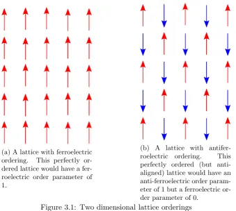
(a) A lattice with ferroelectric ordering. This perfectly or-dered lattice would have a fer-roelectric order parameter of 1.
[image:38.595.153.493.104.408.2](b) A lattice with antifer-roelectric ordering. This perfectly ordered (but anti-aligned) lattice would have an anti-ferroelectric order param-eter of 1 but a ferroelectric or-der parameter of 0.
Figure 3.1: Two dimensional lattice orderings
determiningP =P1−P2 - the antiferroelectric order parameter - and substituting
into equation (3.11).
The polarisation of the system is determined by the global minimum of the free energy, whichever value of polarisation minimises the free energy is the polar-isation that the system relaxes into. As the landscape evolves with temperature and the minima and maxima change in size and location, what was once a global minimum may become only a local minimum or even no longer a minimum at all and the system will pass from one phase to another via a phase transition. As seen in figures (3.2) and (3.3) these can either be a continuous (in the order parame-ter) second order transition or a discontinuous (in the order parameparame-ter) first order transition.
We shall first look for second order transitions in no external field, for this we only require the first three terms of the free energy, so let us examine the derivative ofF to determine where the free energy minima are:
∂F
∂P = 2aP + 4bP
(a) The free energy landscape changing through a second order transition
k
BT/J 0
0.2 0.4 0.6 0.8 1
P
(b) The order parameterP as a function of temperature
Figure 3.2: In the left hand image, the free energy of a system as a func-tion of polarisafunc-tion at various temperatures through a second order (fer-roelectric) transition. Three temperatures are represented, one below the transition temperature (the blue line), one at the transition temperature (black line), one above the transition temperature (red line). This shows how the two minima below the Curie temperature meet at 0 polarisation at the Curie temperature (as the system goes from polarised to unpolarised) and the global minimum of free energy remains at 0 polarisation about the Curie Temperature. In the right hand image we see the order parameter (i.e. the polarisation) undergo a continuous, second order transition as a function of temperature.
This has a minimum when ∂F∂P = 0 when is when either
P = 0 or P2 =−a
2b (3.13)
To classify these as minima or maxima we shall look at the second derivative
∂2F
∂P2 = 2a+ 12bP
2 (3.14)
For P = 0 this gives a second derivative equal to 2a, which means that P = 0 is a minimum fora > 0 and a maximum for a <0, so below TC we want a < 0 and
aboveTC we wanta >0, let us make the assumption [68] that
a=a0(T−Tc) (3.15)
ForP 6= 0, we get
∂2F
∂P2 = 2a−6a =−4a (3.16)
With the definition ofa from equation (3.15) this makes P 6= 0 a minimum
forT < TC as required.
This analysis relies on the assumption thatb >0 otherwise equation (3.13) yields an imaginary value ofP. In the case thatb <0 we must head to higher order terms and requirec >0 in order to have turning points atP 6= 0. The case ofb <0 creates a first order phase transition as seen in figure (3.3).
(a) The free energy landscape changing through a first order transition
kBT/J
0 0.2 0.4 0.6 0.8 1
P
(b) The order parameterP as a function of temperature
Figure 3.3: In the left hand image is the free energy of a system travelling through a first order transition as a function of polarisation. Three tem-peratures are represented, one below the transition temperature (the blue line), one at the transition temperature (black line), one above the transi-tion temperature (red line). This shows how there exist minima in the free energy which are not the global minimum (for example at 0 polarisation below the transition temperature and at non-zero polarisation at the tran-sition temperature). It is the existence of these global minima which cause the discontinuous change in polarisation from non-zero to zero as they do not merge together at zero polarisation as was found in the second order transition case but they remain at non-zero values until they cease to be minima and the polarization which was trapped in a well now relaxes to the global minimum at zero. In the right hand image we see the order parameter of a first order transition.
In this situation we must redefinea
whereT0 is a temperature that is not the transition temperature.
We shall again look at the derivative of the free energy, this time including the term with the third Landau parameter
∂F
∂P = 2aP + 4bP
3+ 6cP5 (3.18)
(3.19) Again, this has a minimum when ∂F∂P = 0, with solutions
P = 0 or P2 =−4b±
√
b2−3ca
3c (3.20)
The system can be manipulated through changing the value of the second landau parameter to display second order transitions (when b > 0) or first order transitions (b < 0), these separate behaviours meet at a tricritical point where
a=b= 0.
The second order transitions are seen to have lower hysteresis losses than first order transitions, while first order transitions have larger entropy changes than second order transitions. This can be explained by the change in order parameter between the paraelectric and ferroelectric phase. In the ferroelectric phase there is a non-zero order parameter, while in the paraelectric phase (in the absence of an ex-ternal field) the order parameter is zero. Second order transitions vary continuously between the zero and non-zero order parameter, while first order transitions have a discontinuous change. A larger change in polarisation results in a larger change in entropy of the system which is why first order transitions exhibit larger entropy changes. However, the large change in polarisation is due to the motion of walls between ferroelectric domains and the energy costs required to cause this movement take away from the total energy applied to the system through the external field and reduce the energy used in the cooling cycle.
Figure (3.4) shows how it is possible to manipulate a system to change the transition temperature between phases, by moving across the phase diagram of the material we may reach a point where second and first order transitions meet and here we would find a tricritical point.
0
40
60
80
P(kBar)
500
600
700
T(K)
AFM
FM
PM
50
70
Figure 3.4: A two-dimensional phase diagram of iron rhodium (FeRh, a material that shall be studied in this thesis) showing how varying pres-sure and temperature may lead this material through ferromagnetic (FM), antiferromagnetic (AFM) or paramagnetic (PM) phases. Adapted from [69]
transitions. This would be the ideal electrocaloric.
3.4
Hysteresis Cycles and Hysteresis Losses
As stated in section (1.3), hysteresis is the effect observed when there is a delay in response from a system with respect to an external stimulus. Domain walls are the cause of hysteresis in a ferroelectric and this explains why no hysteresis is observed in a paraelectric which is free of ferroelectric domains.
A paraelectric system shows no hysteresis, freely aligning itself with an ex-ternally applied field instantly, whereas a ferroelectric system has an intrinsic po-larisation before the application of the external field. Should the field point anti-parallel to this polarisation, the polarisation will not immediately align with the field but there will be a delay until the field is sufficiently large before the polarisa-tion aligns with field as shown previously in figure (1.1) [14] and represented again in figures (3.5a), (3.5b).
for the sake of a reference orientation) then the ferroelectric will be fully polarised in the same direction. This means that all electric dipoles will be oriented in the same direction.
From this starting point, gradually decreasing the field decreases the polari-sation as the dipoles begin to relax into their preferred orientation. There are local regions of dipoles, known as domains, where the dipoles will all preferentially align with each other and between neighbouring domains with non-aligned orientations is a domain wall. The initial large electric field overcomes these domain walls and forces all dipoles to be aligned. As the field is removed the dipoles relax and do-mains with different orientation begin to appear and energy is lost into the system in the creation and movement of the domain walls separating these domains. As the system is a ferroelectric rather than a paraelectric, there will still be a net polarisa-tion, even at zero field and this is due to enough domains having sufficiently similar electric orientations that they produce a net polarisation. Thus in the hysteresis curve we observe that at zero field there is now a residual, intrinsic polarisationPS.
Should the external field now begin to increase in magnitude in the −Z
direction, the polarisation will decrease in value until the field strength reaches a value called the coercive field, EC where the polarisation again returns to zero. In
a relaxor ferroelectric, the domains are isolated polar nano-regions embedded in a matrix of non-polarised material, thus we do not have the same domain wall motion as experienced in a true ferroelectric. This leads to lower values of a coercive field and thinner hysteresis graphs observed than in a pure ferroelectric as less energy is lost to the domain wall motion.
When the field strength increases beyond EC, the polarisation reverses
di-rection and rapidly increases in magnitude as the domain walls move and individual dipoles align along the imposed orientation until the polarisation saturates as before. Decreasing the strength of the field to zero results in a residual polarisation of equivalent strength but in the opposite direction to before. Increasing field strength in the +Z direction results in 0 polarisation at the value of the coercive field again before the polarisation increases superlinearly to saturation.
The hysteresis loss [70] (as seen in figure (3.5)) is simply the difference be-tween the energy required to reverse the internal polarisation of the material and the energy reclaimed from the material as it responds to a reduction in external field.
It is important to avoid the loss associated with the hysteresis effect which is found in first order transitions but is absent in second order transitions [18].
(a) Energy used to establish the field (b) Energy released by collapse of the field
Figure 3.5: The total amount of energy needed to polarise the material is represented by the area inside the hysteresis loop and the area above it up to the maximum value of polarisation. The energy reclaimed is the area outside the hysteresis loop up to the maximum polarisation. The energy represented by the area inside the hysteresis loop is lost in the cycle.
and caloric effects, but we need to create a model with predictive power before we can test this understanding and make progress in our research. The next section will deal with creating models of caloric effects.