warwick.ac.uk/lib-publications
Original citation:
Pollock, Murray, Johansen, Adam M. and Roberts, Gareth O. (2015) On the exact and
ε-strong simulation of (jump) diffusions. Bernoulli, 22 (2). pp. 794-856.
Permanent WRAP URL:
http://wrap.warwick.ac.uk/63814
Copyright and reuse:
The Warwick Research Archive Portal (WRAP) makes this work by researchers of the
University of Warwick available open access under the following conditions. Copyright ©
and all moral rights to the version of the paper presented here belong to the individual
author(s) and/or other copyright owners. To the extent reasonable and practicable the
material made available in WRAP has been checked for eligibility before being made
available.
Copies of full items can be used for personal research or study, educational, or not-for-profit
purposes without prior permission or charge. Provided that the authors, title and full
bibliographic details are credited, a hyperlink and/or URL is given for the original metadata
page and the content is not changed in any way.
A note on versions:
The version presented in WRAP is the published version or, version of record, and may be
cited as it appears here.
DOI:10.3150/14-BEJ676
On the exact and
ε
-strong simulation of
(jump) diffusions
M U R R AY P O L L O C K*, A DA M M . J O H A N S E N**and G A R E T H O . RO B E RT S†
Department of Statistics, University of Warwick, Coventry, CV4 7AL, United Kingdom.
E-mail:*[email protected];**[email protected];†[email protected]
This paper introduces a framework for simulating finite dimensional representations of (jump) diffusion sample paths over finite intervals, without discretisation error (exactly), in such a way that the sample path can be restored at any finite collection of time points. Within this framework we extend existing exact algo-rithms and introduce novel adaptive approaches. We consider an application of the methodology developed within this paper which allows the simulation of upper and lower bounding processes which almost surely constrain (jump) diffusion sample paths to any specified tolerance. We demonstrate the efficacy of our ap-proach by showing that with finite computation it is possible to determine whether or not sample paths cross various irregular barriers, simulate to any specified tolerance the first hitting time of the irregular barrier and simulate killed diffusion sample paths.
Keywords:adaptive exact algorithms; barrier crossing probabilities; Brownian path space probabilities; exact simulation; first hitting times; killed diffusions
1. Introduction
Diffusions and jump diffusions are widely used across a number of application areas. An exten-sive literature exists in economics and finance, spanning from the seminal Black–Scholes model [10,25,26] to the present [4,16]. Other applications can be easily found within the physical [29] and life sciences [18,19] to name but a few. A jump diffusionV:R→Ris a Markov process. In this paper, we consider jump diffusions defined as the solution to a stochastic differential equation (SDE) of the form (denotingVt−:=lims↑tVs),
dVt=β(Vt−)dt+σ (Vt−)dWt+dJtλ,μ, V0=v∈R, t∈ [0, T], (1)
whereβ:R→R andσ:R→R+ denote the (instantaneous) drift and diffusion coefficients, respectively, Wt is a standard Brownian motion and Jtλ,μ denotes a compound Poisson
pro-cess.Jtλ,μ is parameterised with (finite) jump intensity λ:R→R+ and jump size coefficient
μ:R→Rwith jumps distributed with densityfμ. All coefficients are themselves (typically)
dependent onVt. Regularity conditions are assumed to hold to ensure the existence of a unique
non-explosive weak solution (see, e.g., [28,30]). To apply the methodology developed within this paper we primarily restrict our attention to univariate diffusions and require a number of addi-tional conditions on the coefficients of (1), details and a discussion of which can be found in Section2.
Motivated by the wide range of possible applications we are typically interested (directly or indirectly) in the measure ofV on the path space induced by (1), denotedTv0,T. AsTv0,T is typ-ically not explicitly known, in order to compute expected valuesETv
0,T[h(V )]for various test
functionsh:R→R, we can construct a Monte Carlo estimator. In particular, if it is possible to draw independentlyV(1), V(2), . . . , V(n)∼Tv0,T then by applying the strong law of large num-bers we can construct a consistent estimator of the expectation (unbiasedness follows directly by linearity),
w.p. 1: lim
n→∞
1
n n i=1
hV(i)=ETv
0,T
h(V ). (2)
Furthermore, providedVTv
0,T[h(V )] =:σ 2
h <∞, by application of the central limit theorem we
have,
lim
n→∞
√
n
ETv
0,T
h(V )−1 n
n i=1
hV(i)
D
=ξ, whereξ∼N0, σh2. (3)
Unfortunately, as diffusion sample paths are infinite dimensional random variables it isn’t pos-sible to draw an entire sample path fromTv0,T – at best we can hope to simulate some finite dimensional subset of the sample path, denotedVfin (we further denote the remainder of the sample path byVrem:=V \Vfin). Careful consideration has to be taken as to how to simulate
Vfinas any numerical approximation impacts the unbiasedness and convergence of the resulting Monte Carlo estimator (2), (3). Equally, consideration has to be given to the form of the test function,h, to ensure it’s possible to evaluate it givenVfin.
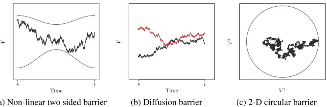
To illustrate this point we consider some possible applications. In Figure1(a), (b) and (c) we are interested in whether a simulated sample pathV ∼Tv0,T, crosses some barrier (i.e., for some setAwe haveh(V ):=1(V ∈A)). Note that in all three cases in order to evaluatehwe would require some characterisation of the entire sample path (or some further approximation) and even for diffusions with constant coefficients and simple barriers this is difficult. For instance, as illustrated in Figure1(c), even in the case whereTv0,T is known (e.g., whenTv0,T is Wiener
[image:3.488.67.401.440.550.2](a) Non-linear two sided barrier (b) Diffusion barrier (c) 2-D circular barrier
measure) and the barrier is known in advance and has a simple form, there may still not exist any exact approach to evaluate whether or not a sample path has crossed the barrier.
Diffusion sample paths can be simulated approximately at a finite collection of time points bydiscretisation[21,24,30], noting that as Brownian motion has a Gaussian transition density then over short intervals the transition density of (1) can be approximated by that of an SDE with fixed coefficients (by a continuity argument). This can be achieved by breaking the interval the sample path is to be simulated over into a fine mesh (e.g., of sizet), then iteratively (at each mesh point) fixing the coefficients and simulating the sample path to the next mesh point. For instance, in anEulerdiscretisation [21] of (1), the sample path is propagated between mesh points as follows (whereξ∼N(0, t )andμt∼fμ(·;Vt)),
Vt+t =
Vt+β(Vt)t+σ (Vt)ξ, w.p. exp
−λ(Vt)t
,
Vt+β(Vt)t+σ (Vt)ξ+μt, w.p. 1−exp
−λ(Vt)t
. (4)
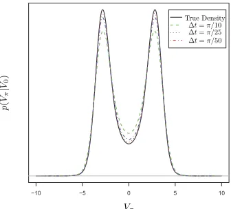
[image:4.488.173.341.393.545.2]It is hoped the simulated sample path (generated approximately at a finite collection of mesh points) can be used as a proxy for an entire sample path drawn exactly fromTv0,T. More complex discretisation schemes exist (e.g., by exploiting Itô’s lemma to make higher order approximations or by local linearisation of the coefficients [24,30]), but all suffer from common problems. In particular, minimising the approximation error (by increasing the mesh density) comes at the expense of increased computational cost, and further approximation or interpolation is needed to obtain the sample path at non-mesh points (which can be non-trivial). As illustrated in Figure2, even when our test function h only requires the simulation of sample paths at a single time point, discretisation introduces approximation error resulting in the loss of unbiasedness of our Monte Carlo estimator (2). IfTv0,T has a highly non-linear drift or includes a compound jump process orhrequires simulation of sample paths at a collection of time points then this problem is exacerbated. In the case of the examples in Figure1, mesh based discretisation schemes don’t sufficiently characterise simulated sample paths for the evaluation ofh.
Recently, a new class ofExact Algorithmsfor simulating sample paths at finite collections of time points without approximation error have been developed for both diffusions [5,6,9,14] and jump diffusions [13,17,20]. These algorithms are based on rejection sampling, noting that sample paths can be drawn from the (target) measureTv0,T by instead drawing sample paths from an equivalent proposal measurePv0,T, and accepting or rejecting them with probability proportional to the Radon–Nikodým derivative ofTv0,T with respect toPv0,T. However, as with discretisation schemes, given a simulated sample path at a finite collection of time points subsequent simulation of the sample path at any other intermediate point may require approximation or interpolation and may not be exact. Furthermore, we are again unable to evaluate test functions of the type illustrated in Figure1.
The key contribution of this paper is the introduction of a novel mathematical framework for constructing exact algorithms which addresses this problem. In particular, instead of exactly simulating sample paths at finite collections of time points, we focus on the extended notion of simulatingskeletonswhich in addition characterise the entire sample path.
Definition 1 (Skeleton). A skeleton(S)is a finite dimensional representation of a diffusion sam-ple path(V ∼Tv0,T),that can be simulated without any approximation error by means of a proposal sample path drawn from an equivalent proposal measure(Pv0,T) and accepted with
probability proportional to dT
v
0,T dPv
0,T
(V ),which is sufficient to restore the sample path at any
fi-nite collection of time points exactly with fifi-nite computation whereV|S∼Pv0,T|S.A skeleton typically comprises information regarding the sample path at a finite collection of time points and path space information which ensures the sample path is almost surely constrained to some compact interval.
Methodology for simulating skeletons (the size and structure of which is dependent on ex-ogenous randomness) is driven by both computational and mathematical considerations (i.e., we need to ensure the required computation is finite and the skeleton is exact). Central to both no-tions is that the path space of the proposal measurePv0,T can be partitioned (into a set oflayers), and that the layer to which any sample path belongs to can be simulated.
Definition 2 (Layer). A layerR(V ),is a function of a diffusion sample pathV ∼Pv0,T which determines the compact interval to which any particular sample pathV (ω)is constrained.
To illustrate the concept of a layer and skeleton, we could, for instance, haveR(V )=inf{i∈ N: ∀u∈ [0, T], Vu∈ [v−i, v+i]}andS= {V0=v, VT =w, R(V )=1}.
We show that a valid exact algorithm can be constructed if it is possible to partition the pro-posal path space into layers, simulate unbiasedly to which layer a propro-posal sample path belongs and then, conditional on that layer, simulate a skeleton. Our exact algorithm framework for sim-ulating skeletons is based on three principles for choosing a proposal measure and simsim-ulating a path space layer:
Principle 1 (Layer construction). The path space of the process of interest,can be partitioned and the layer to which a proposal sample path belongs can be unbiasedly simulated,R(V )∼ R:=Pv
Principle 2 (Proposal exactness). Conditional onV0,VT andR(V ),we can simulate any
fi-nite collection of intermediate points of the trajectory of the proposal diffusion exactly,V ∼ Pv
0,T|R−1(R(V )).
Together Principles1and2ensure it is possible to simulate a skeleton. However, in addition we want to characterise the entire sample path and so we construct exact algorithms with the following additional principle.
Principle 3 (Path restoration). Any finite collection of intermediate(inference)points, condi-tional on the skeleton,can be simulated exactly,Vt1, . . . , Vtn∼P
v 0,T|S.
In developing a methodological framework for simulating exact skeletons of (jump) diffusion sample paths we are able to present a number of significant extensions to the existing literature on exact algorithms [5,6,13,20]. In particular, we present novel exact algorithm constructions requiring the simulation of fewer points of the proposal sample path in order to evaluate whether to accept or reject (in effect a Rao–Blackwellisation of EA3 for diffusions [6], which we term the Unbounded Exact Algorithm (UEA), and a Rao–Blackwellisation of the Jump Exact Algo-rithms (JEAs) for jump diffusions [13,20], which we term the Bounded Jump Exact Algorithm (BJEA) and Unbounded Jump Exact Algorithm (UJEA), resp.) – all of which we recommend are adopted in practice instead of the existing equivalent exact algorithm. Furthermore, we extend both existing and novel exact algorithms to satisfy Principle3, enabling the further simulation of a proposed sample pathafterit has been accepted, which hitherto has not been possible except under the limiting conditions imposed in EA1 [5].
Although in the context of a particular application we do not necessarily require the ability to further simulate a proposal sample path after acceptance (e.g., particle filtering for partially observed jump diffusions [31], in which only the end point of each sample path is required), to tackle the type of problem in which we do require that Principle3 is satisfied (e.g., in the examples outlined Figure1) we introduce a novel class ofAdaptive Exact Algorithms (AEAs) for both diffusions and jump diffusions (which are again in effect a Rao–Blackwellisation of the Unbounded Exact Algorithm (UEA) requiring fewer points of the proposal sample path in order to evaluate whether to accept or reject).
In summary, the main contributions of this paper are as follows:
– A mathematical framework for constructing exact algorithms for both diffusions and jump diffusions, enabling improvements to existing exact algorithms, extension of existing exact algorithms to satisfy Principle3and a new class of adaptive exact algorithms (see Sections3
and4).
– Methodology for the ε-strong simulation of diffusion and jump diffusion sample paths, along with a novel exact algorithm based on this construction (see Sections5and8). – New methodology for constructing Monte Carlo estimators to compute irregular barrier
crossing probabilities, simulating first hitting times to any specified tolerance and simulating killed diffusion sample path skeletons (see Sections5and9). This work is reliant on the methodological extensions of Sections3–5and is presented along with examples based on the illustrations in Figure1.
We also make a number of other contributions which are necessary for the implementation of our methodology. In particular, we detail how to simulate unbiasedly events of probability corre-sponding to various Brownian path space probabilities (see Section6); and, we make significant extensions to existingε-strong methodology enabling the initialisation of the algorithm and en-suring exactness (see Sections5and8).
This paper is organised as follows: in Section2, we detail conditions sufficient to establish results necessary for applying the methodology in this paper. In Sections3 and4, we outline our exact algorithm framework for diffusions and jump diffusions, respectively, presenting the resulting UEA, Bounded Jump Exact Algorithm (BJEA), Unbounded Jump Exact Algorithm (UJEA) and AEAs. In Section5, we apply our methodology enabling theε-strong simulation of (jump) diffusions. We extend existing layered Brownian bridge constructions in Section7, introducing novel constructions for the AEAs in Section8(both of which rely on novel Brownian path space simulation results which are summarised in Section6). Finally in Section9, we revisit the examples outlined in Figure1to which we apply our methodology.
2. Preliminaries
In order to apply the methodology in this paper, we require conditions in order to establish Results1–4which we introduce below. To present our work in some generality we assume Con-ditions1–5hold (see below) along with some indication of why each is required. However, these conditions can be difficult to check and so in Section2.1we discuss verifiable sufficient condi-tions under which Results1–4hold.
Condition 1 (Solutions). The coefficients of(1)are sufficiently regular to ensure the existence of a unique,non-explosive,weak solution.
Condition 2 (Continuity). The drift coefficientβ∈C1.The volatility coefficientσ ∈C2and is strictly positive.
Condition 3 (Growth bound). We have that∃K >0such that|β(x)|2+ |σ (x)|2≤K(1+ |x|2)
Condition 4 (Jump rate). λis non-negative and locally bounded.
Conditions2and3are sufficient to allow us to transform our SDE in (1) into one with unit volatility,
Result 1 (Lamperti transform [24], Chapter 4.4). Letη(Vt)=:Xt be a transformed process,
whereη(Vt):= Vt
v∗ 1/σ (u)du (wherev∗ is an arbitrary element in the state space ofV).We
denote byψ1, . . . , ψNT as the jump times in the interval[0, T],ψ0:=0,ψNT+1− :=ψNT+1:= T and Nt :=
i≥11{ψi ≤t}a Poisson jump counting process.Further denoting by Vcts the
continuous component ofV and applying Itô’s formula for jump diffusions to finddXt we have
(whereμt∼fμ(·;Vt−)=fμ(·;η−1(Xt−))),
dXt =
ηdVtcts+ηdVtcts2/2+η[Vt−+μt] −η(Vt−)
dNt
(5)
=
β(η−1(Xt−)) σ (η−1(X
t−))
−σ(η−1(Xt−))
2
α(Xt−)
dt+dWt+
ηη−1(Xt−)+μt
−Xt−
dNt
dJtλ,ν
.
This transformation is typically possible for univariate diffusions and for many multivariate diffusions [1]. A significant class of multivariate diffusions can be simulated by direct application of our methodology, and ongoing work is aimed at extending these methodologies more broadly to multivariate diffusions (see [35]).
In the remainder of this paper, we assume (without loss of generality) that we are dealing with transformed SDEs with unit volatility coefficient as in (5). As such, we introduce the follow-ing simplifyfollow-ing notation. In particular, we denote byQx0,T the measure induced by (5) and by Wx
0,T the measure induced by the driftless version of (5). We defineA(u):= u
0 α(y)dyand set φ(Xs):=α2(Xs)/2+α(Xs)/2. Ifλ=0 in (5) thenWx0,T is Wiener measure. Furthermore, we
impose the following final condition.
Condition 5 (). There exists a constant >−∞such that≤φ.
It is necessary for this paper to establish that the Radon–Nikodým derivative of Qx0,T with respect toWx0,T exists (Result2) and can be bounded on compact sets (Results3and4) under Conditions1–5.
Result 2 (Radon–Nikodým derivative [28,30]). Under Conditions 1–4, the Radon–Nikodým derivative ofQx0,T with respect toWx0,T exists and is given by Girsanov’s formula:
dQx0,T
dWx0,T(X)=exp
T 0
α(Xs)dWs−
1 2
T 0
α2(Xs)ds
As a consequence of Condition2,we haveA∈C2and so we can apply Itô’s formula to remove the stochastic integral,
dQx0,T
dWx0,T(X)=exp A(XT)−A(x)−
T 0
φ(Xs)ds− NT i=1
A(Xψi)−A(Xψi−)
. (7)
In the particular case where we have a diffusion(λ=0),
dQx0,T
dWx0,T(X)=exp
A(XT)−A(x)− T
0
φ(Xs)ds
. (8)
Result 3 (Quadratic growth). As a consequence of Condition3,we have thatAhas a quadratic growth bound and so there exists someT0<∞such that∀T ≤T0:
c(x, T ):=
Rexp
A(y)−(y−x) 2
2T
dy <∞. (9)
Throughout this paper, we rely on the fact that upon simulating a path space layer (see Def-inition2) then∀s∈ [0, T]φ(Xs)is bounded, however this follows directly from the following
result.
Result 4 (Local boundedness). By Condition2,αandαare bounded on compact sets.In par-ticular,suppose∃, υ∈Rsuch that∀t∈ [0, T],Xt(ω)∈ [, υ] ∃LX:=L(X(ω))∈R, UX:= U (X(ω))∈Rsuch that∀t∈ [0, T],φ(Xt(ω))∈ [LX, UX].
2.1. Verifiable Sufficient Conditions
As discussed in [28], Theorem 1.19, to ensure Condition1 it is sufficient to assume that the coefficients of (1) satisfy the following linear growth and Lipschitz continuity conditions for some constantsC1, C2<∞(recalling thatfμis the density of the jump sizes),
β(x)2+σ (x)2+
R
fμ(z;x) 2
λ(dz)≤C1
1+ |x|2, ∀x∈R, (10)
β(x)−β(y)2
+σ (x)−σ (y)2
+
R
fμ(z;x)−fμ(z;y) 2
λ(dz)
(11)
≤C2|x−y|2, ∀x, y∈R.
(10) and (11) together with Condition 2 are sufficient for the purposes of implementing the methodology in this paper (in particular, Conditions1,3,4and5will hold in this situation) but are not necessary. Although easy to verify, (10) and (11) are somewhat stronger than necessary for our purposes and so we impose Condition1instead.
admits a unique weak solution [27] and so Condition1holds. In particular, the methodology in this paper will hold under Conditions2,3and5.
3. Exact Simulation of Diffusions
In this section, we outline how to simulate skeletons for diffusion sample paths (we will return to jump diffusions in Section4) which can be represented (under the conditions in Section2and following the transformation in (5)), as the solution to SDEs with unit volatility,
dXt=α(Xt)dt+dWt, X0=x∈R, t∈ [0, T]. (12)
As discussed in Section1, exact algorithms are a class of rejection samplers operating on diffu-sion path space. In this section, we begin by reviewing rejection sampling and outline an (ide-alised) rejection sampler originally proposed in [9] for simulating entire diffusion sample paths. However, for computational reasons this idealised rejection sampler can’t be implemented so instead, with the aid of new results and algorithmic step reordering, we address this issue and construct a rejection sampler for simulating sample path skeletons which only requires finite computation. A number of existing exact algorithms exist based on this approach [5,6,9], how-ever, in this paper we present two novel algorithmic interpretations of this rejection sampler. In Section3.1, we present the Unbounded Exact Algorithm (UEA), which is a methodological extension of existing exact algorithms [6], requiring less of the proposed sample path to be sim-ulated in order to evaluate acceptance or rejection. Finally, in Section3.2we introduce the novel Adaptive Unbounded Exact Algorithm (AUEA), which as noted in theIntroduction, is well suited to problems in which further simulation of a proposed sample pathafterit has been accepted is required.
Rejection sampling[34] is a standard Monte Carlo method in which we can sample from some (inaccessible) target distributionπ by means of an accessible dominating distributiongwith re-spect to whichπ is absolutely continuous with bounded Radon–Nikodým derivative. In particu-lar, if we can find a boundMsuch that supxddπg(x)≤M <∞, then drawingX∼gand accepting
the draw (settingI=1) with probabilityPg(X):=M1 ddπg(X)∈ [0,1]then(X|I=1)∼π.
Similarly, we could simulate sample paths from our target measure (the measure induced by (12) and denotedQx0,T) by means of a proposal measure which we can simulate proposal sample paths from, provided a bound for the Radon–Nikodým derivative can be found. A natural equivalent measure to choose as a proposal is Wiener measure (Wx0,T, as (12) has unit volatil-ity). In particular, drawingX∼Wx0,T and accepting the sample path(I=1)with probability
PWx
0,T(X):= 1 M
dQx0,T dWx
0,T
(X)∈ [0,1](where dQ
x
0,T dWx
0,T
(X)is as given in (8)) then(X|I =1)∼Qx0,T.
On average sample paths would be accepted with probabilityPWx
0,T :=EWx0,T[PWx0,T(X)].
How-ever, the functionA(XT)in (8) only has a quadratic growth bound (see Result3), so typically no
appropriate bound (M <∞) exists.
To remove the unbounded functionA(XT)from the acceptance probability, one can use Biased
Definition 3. Biased Brownian motion is the process Zt D=(Wt|W0=x, WT :=y ∼h) with
measureZx0,T,wherex, y∈R,t ∈ [0, T] andh is defined as(by Result3 we have∀T ≤T0, h(y;x, T )is integrable),
h(y;x, T ):= 1 c(x, T )exp
A(y)−(y−x) 2
2T
. (13)
Theorem 1 (Biased Brownian motion [9], Proposition 3). Qx0,T is equivalent to Zx0,T with Radon–Nikodým derivative:
dQx0,T
dZx0,T (X)∝exp
−
T 0
φ(Xs)ds
. (14)
Sample paths can be drawn fromZx0,T in two steps by first simulating the end point XT =: y∼h (althoughh doesn’t have a tractable form, a rejection sampler with Gaussian proposal can typically be constructed) and then simulating the remainder of the sample path in(0, T )
from the law of a Brownian bridge,(X|X0=x, XT =y)∼Wx,y0,T. We can now construct an
(idealised) rejection sampler to draw sample paths fromQx0,T as outlined in Algorithm1, noting that as infu∈[0,T]φ(Xu)≥(see Condition5) we can identifyand chooseM:=exp{−T}
to ensurePZx
0,T(X)∈ [0,1].
Unfortunately, Algorithm1 can’t be implemented directly as it isn’t possible to draw entire sample paths fromWx,y0,T in Step 1(b) (they’re infinite dimensional random variables) and it isn’t possible to evaluate the integral expression in the acceptance probability in Step 2.
The key to constructing an implementable algorithm (which requires only finite computation), is to note that by first simulating some finite dimensional auxiliary random variableF ∼F(the details of which are in Sections3.1and3.2), an unbiased estimator of the acceptance probability can be constructed which can be evaluated using only a finite dimensional subset of the proposal sample path. As such, we can use the simulation ofF to inform us as to what finite dimensional subset of the proposal sample path to simulate (Xfin∼Wx,y0,T|F) in Step 1(b) in order to evaluate the acceptance probability. The rest of the sample path can be simulated as requiredafterthe acceptance of the sample path from the proposal measure conditional on the simulations per-formed,Xrem∼Wx,y0,T|(Xfin, F )(noting thatX=Xfin∪Xrem). The synthesis of this argument is presented in Algorithm2.
Note that Algorithm2Step 5 is separated from the rest of the algorithm and asterisked. This convention is used within this paper to indicate the final step within an exact algorithm, which
Algorithm 1Idealised Rejection Sampler [9] 1. SimulateX∼Zx0,T,
(a) SimulateXT =:y∼h.
(b) SimulateX(0,T )∼Wx,y0,T.
2. With probabilityPZx
0,T(X)=exp{− T
0 φ(Xs)ds} ·exp{T}accept, else reject and return
Algorithm 2Implementable Exact Algorithm [5,9] 1. SimulateXT =:y∼h.
2. SimulateF∼F.
3. SimulateXfin∼Wx,y0,T|F. 4. With probabilityPZx
0,T|F(X)accept, else reject and return to Step 1.
5. ∗SimulateXrem∼Wx,y0,T|(Xfin, F ).
cannot be conducted in its entirety as it involves simulating an infinite dimensional random vari-able. However, as noted in the introductory remarks to this section, our objective is to simulate a finite dimensional sample path skeleton, with which we can simulate the accepted sample path at any other finite collection of time points without error. This final step simply indicates how this subsequent simulation may be conducted.
In conclusion, although it isn’t possible to simulate entire sample paths fromQx0,T, it is pos-sible to simulate exactly a finite dimensional subset of the sample path, characterised by its skeletonS(X):= {X0, Xfin, XT, F}. Careful consideration has to be taken to constructFwhich
existing exact algorithms [5,6,9] achieve by applying Principles1 and2. However, no existing exact algorithm addresses how to constructFunder the conditions in Section2to additionally perform Algorithm2Step 5. We address this in Sections3.1and3.2.
In the next two sections, we present two distinct, novel interpretations of Algorithm2. In Sec-tion3.1, we present the UEA which is a methodological extension of existing exact algorithms and direct interpretation of Algorithm2. In Section3.2, we introduce the AUEA which takes a recursive approach to Algorithm2Steps 2, 3 and 4.
3.1. Bounded and Unbounded Exact Algorithms
In this section, we present the Unbounded Exact Algorithm (UEA) along with the Bounded Exact Algorithm (BEA) (which can viewed as a special case of the UEA) by revisiting Algorithm2and considering how to construct a suitable finite dimensional random variableF ∼F.
As first noted in [5], it is possible to construct and simulate the random variableF required in Algorithm2, providedφ(X[0,T])can be bounded above and below. It was further noted in [6]
that if a Brownian bridge proposal sample path was simulated along with an interval in which is was contained, and that conditional on this intervalφ(X[0,T])was bounded above and below,
thenF could similarly be constructed and simulated. Finding a suitable set of information that establishes an interval in which φ(X[0,T])is contained (by means of finding and mapping an
interval in which the sample path X[0,T] is contained), is the primary motivation behind the
notion of a sample path layer (see Definition2). In this paper, we discuss more than one layer construction (see Sections7and8), both of which complicate the key ideas behind the UEA and so layers are only discussed in abstract terms at this stage.
Further to [6], we note that φ(X[0,T])is bounded on compact sets (see Result4) and so if,
(see Principle1, denotingR:=R(X)∼Ras the simulated layer the precise details of which are given in Section7), then an upper and lower bound forφ(X[0,T])can always be found conditional
on this layer (UX∈RandLX∈R, resp.). As such, we have for all test functionsH∈Cb,
EZx
0,T
PZx
0,T(X)·H (X)
=EhEWx,y
0,T
PZx
0,T(X)·H (X)
(15)
=EhEREWx,y
0,T|R
PZx
0,T(X)·H (X)
,
recalling that,
PZx
0,T(X)=exp
−
T 0
φ(Xs)ds
·eT. (16)
Proceeding in a similar manner to [7] to construct our finite dimensional estimator we consider a Taylor series expansion of the exponential function in (16),
PZx
0,T(X)=e
−(LX−)T ·e−(UX−LX)Texp T
0
UX−φ(Xs)ds
(17)
=e−(LX−)T ·
∞ j=0
e−(UX−LX)T[(U
X−LX)T]j j!
T 0
UX−φ(Xs) (UX−LX)T
ds j
,
again employing methods found in [7], we note that if we letKR be the law ofκ∼Poi((UX−
LX)T ),Uκ the distribution of(ξ1, . . . , ξκ) iid
∼U[0, T]we have,
PZx
0,T(X)=e
−(LX−)T ·E
KR T
0
UX−φ(Xs)
(UX−LX)T
ds κ
X
(18)
=e−(LX−)T ·E
KR
EUκ κ
i=1
UX−φ(Xξi)
UX−LX X X .
The key observation to make from (18) is that the acceptance probability of a sample pathX∼ Zx
0,T can be evaluated without using the entire sample path, and can instead be evaluated using a
finite dimensional realisation,Xfin. Simulating a finite dimensional proposal as suggested by (18) and incorporating it within Algorithm2results directly in the UEA presented in Algorithm3. A number of alternate methods for simulating unbiasedly layer information (Step 2), layered Brownian bridges (Step 4), and the sample path at further times after acceptance (Step 6), are given in Section7.
Algorithm 3Unbounded Exact Algorithm (UEA) 1. Simulate skeleton end pointXT =:y∼h.
2. Simulate layer informationR∼R.
3. With probability(1−exp{−(LX−)T})reject path and return to Step 1.
4. Simulate skeleton points(Xξ1, . . . , Xξκ)|R,
(a) Simulateκ∼Poi((UX−LX)T )and skeleton timesξ1, . . . , ξκ iid
∼U[0, T]. (b) Simulate sample path at skeleton timesXξ1, . . . , Xξκ ∼W
x,y 0,T|R.
5. With probability κi=1[(UX−φ(Xξi))/(UX−LX)], accept entire path, else reject and
return to Step 1.
6. ∗SimulateXrem∼(κi=+11WXξi−1,Xξi
ξi−1,ξi )|R.
unnecessary simulation of the rejected sample path. In particular, the UEA requires simulation of fewer points of the proposal sample path in order to evaluate whether to accept or reject.
The skeleton of an accepted sample path includes any information simulated for the purpose of evaluating the acceptance probability (any subsequent simulation must be consistent with the skeleton). As such, the skeleton is composed of terminal points, skeletal points (Xξ1, . . . , Xξκ) and layerR(denotingξ0:=0 andξκ+1:=T),
SUEA(X):=(ξi, Xξi)κi=+01, R
. (19)
After simulating an accepted sample path skeleton, we may want to simulate the sample path at further intermediate points. In the particular case in whichφ(X[0,T])is almost surely bounded,
there is no need to simulate layer information in Algorithm3, the skeleton can be simulated from the law of a Brownian bridge and given the skeleton we can simulate further intermediate points of the sample path from the law of a Brownian bridge (so we satisfy Principle3). This leads to theExact Algorithm1 (EA1) proposed in [5], which we term the BEA,
SBEA(X):=(ξi, Xξi)κi=+01
. (20)
A second exact algorithm (EA2) was also proposed in [5] (the details of which we omit from this paper), in which simulating the sample path at further intermediate points after accepting the sample path skeleton was possible by simulating from the law of two independent Bessel bridges. However, EA1 (BEA) and EA2 both have very limited applicability and are the only existing exact algorithms which directly satisfy Principle3.
(denotingRX[a,b]as the layer for the sub-interval[a, b] ⊆ [0, T]),
SUEA (X):=
(ξi, Xξi) κ+1 i=0, R,
R[ξi−1,ξi] X
κ+1 i=1
A
(21)
≡(ξi, Xξi)κi=+01,
R[ξi−1,ξi] X
κ+1 i=1
B
.
The augmented skeleton allows the sample path to be decomposed into conditionally independent paths between each of the skeletal points and so the layer R no longer imparts information across the entire interval[0, T]. In particular, the sets in (21) are equivalent in the sense that Wx,y
0,T|A=W x,y
0,T|B. As such, simulating the sample path at further times after acceptance as in
Algorithm3Step 6 is direct,
Xrem∼Wx,y0,T|SUEA = κ+1 i=1
WXξi−1,Xξi
ξi−1,ξi |R
[ξi−1,ξi]
X
. (22)
3.1.1. Implementational Considerations – Interval Length
It transpires that the computational cost of simulating a sample path scales worse than linearly with interval length. However, this scaling problem can be addressed by exploiting the fact that sample paths can be simulated by successive simulation of sample paths of shorter length over the required interval by applying the strong Markov property, noting the Radon–Nikodým derivative in (8) decomposes as follows (for anyt∈ [0, T]),
dQx0,T
dWx0,T(X)=exp
A(Xt)−A(x)− t
0
φ(Xs)ds
(23)
×exp
A(XT)−A(Xt)− T
t
φ(Xs)ds
.
3.2. Adaptive Unbounded Exact Algorithm
Within this section, we outline a novel Adaptive Unbounded Exact Algorithm (AUEA). To mo-tivate this, we revisit Algorithm2noting that the acceptance probability (16) of a sample path
X∼Zx0,T can be rewritten as follows,
PZx
0,T(X)=exp
−
T 0
φ(Xs)−LX
ds
·e−(LX−)T =: ˜P
Zx
0,T|R(X)·e
−(LX−)T. (24)
Now following Algorithm3, after simulating layer information (Step 2) and conditionally ac-cepting the proposal sample path in the first (inexpensive) part of the multi-step rejection sampler (Step 3) the probability of accepting the sample path is,
˜
PZx
0,T|R(X)∈
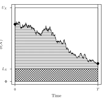
Figure 3. Example trajectory ofφ(X)whereX∼Wx,y0,T|R(X).
Reinterpreting the estimator in (18) in light of (25) and with the aid of Figure3, we are exploiting the fact thatP˜Zx
0,T|R(X)is precisely the probability a Poisson process of intensity 1 on the graph GA:= {(x, y)∈ [0, T] × [LX,∞): y≤φ(x)} contains no points. As this is a difficult set in
which to simulate a Poisson process (we don’t even know the entire trajectory ofX), we are instead simulating a Poisson process of intensity 1 on the larger graphGP := [0, T]×[LX, UX] ⊇ GA (which is easier asUX−LX is a constant), and then conducting Poisson thinning by first
computingφ(X)at the finite collection of time points of the simulated Poisson process and then determining whether or not any of the points lie inGA(accepting the entire sample path if there
are no Poisson points inGA⊆GP). This idea was first presented in [5] and formed the basis of
the Bounded Exact Algorithm (BEA) discussed in Section3.1.
As an aside, it should be noted that conditional acceptance of the proposal sample path with probability e−(LX−)T in Algorithm3Step 3 is simply the probability that a Poisson process
of intensity 1 has no points on the graph GR:= [0, T] × [, LX](the crosshatched region in
Figure3).
In some settingsGP can be much larger thanGA and the resulting exact algorithm can be
in-efficient and computationally expensive. In this section, we propose anadaptivescheme which exploits the simulation of intermediate skeletal points of the proposal sample path in Algorithm3
Step 4. In particular, note that each simulated skeletal point implicitly provides information re-garding the layer the sample path is contained within in both the sub-interval before and after it. As such, by simulating each point separately we can use this information to construct a modified bounding regionGPM such thatGA⊆GMP ⊆GP, composed of a Poisson process with piecewise
constant intensity, for the simulation of the remaining points.
In Algorithm3Step 4(a), we simulate a Poisson process of intensityXT :=(UX−LX)T
on the interval[0, T]to determine the skeletal points (ξ1, . . . , ξκ). Alternatively we can exploit
the exponential waiting time property between successive events [23]. In particular, denoting
T1, . . . , Tκas the time between each eventξ1, . . . , ξκ, then the timing of the events can be
simu-lated by successive Exp(X)waiting times whileiTi≤T.
the mid-point of the interval will contain more information about the layer structure of the entire sample path. As such, there is an advantage in simulating these points first. If we begin at the interval mid-point (T /2), we can find the skeletal point closest to it by simulating an Exp(2X)
random variable,τ (we are simulating the first point ateitherside of the mid-point). As such, the simulated point (denotedξ) will be with equal probability at either T /2−τ orT /2+τ. Considering this in the context of (25), upon simulatingξ we have simply broken the acceptance probability into the product of three probabilities associated with three disjoint sub-intervals, the realisation of the sample path atXξ providing a binary unbiased estimate of the probability
corresponding to the central sub-interval (where the expectation is with respect tou∼U[0,1]),
˜
PZx
0,T|R,Xξ(X)=exp
−
T /2−τ 0
φ(Xs)−LX
ds− T
T /2+τ
φ(Xs)−LX ds (26) ×E 1
u≤UX−φ(Xξ) UX−LX
Xξ
.
If the central sub-interval is rejected, the entire sample path can be discarded. However, if it is accepted then the acceptance of the entire sample path is conditional on the acceptance ofboth the left- and right-hand sub-intervals in (26), each of which has the same structural form as we originally had in (25). As such, for each we can simply iterate the above process until we have exhausted the entire interval[0, T].
As outlined above, our approach is an algorithmic reinterpretation, but otherwise identical, to Algorithm3. However, we now have the flexibility to exploit the simulated skeletal pointXξ, to
simulate new layer information for the remaining sub-intervals conditional on the existing layer
RX(which we detail in Section8). In particular, considering the left-hand sub-interval in (26),
we can find new layer information (denotedR[X0,ξ]) which will contain tighter bound information regarding the sample path (X≤[X0,ξ]≤X[0,ξ](ω)≤υX[0,ξ]≤υX) and so (as a consequence
of Result4) can be used to compute tighter bounds for φ(X[0,ξ])(denoted UX[0,ξ](≤UX)and L[X0,ξ](≥LX)),
˜
P[0,ξ]
Zx
0,T|R
[0,ξ] X ,Xξ
(X)
=exp
−
T /2−τ 0
φ(Xs)−LX ds (27) =exp
−L[X0,ξ]−LX
·
T
2 −τ
·exp
−
T /2−τ 0
φ(Xs)−L[X0,ξ]
ds
.
The left-hand exponential in (27) is a constant and it is trivial to immediately reject the entire path with the complement of this probability. The right-hand exponential of (27) has the same form as (25) and so the same approach as outlined above can be employed, but over the shorter interval
[0, T /2−τ]and with the lower rateX[0,ξ](:=UX[0,ξ]−L[X0,ξ]≤X). As a consequence, the
Algorithm 4Adaptive Unbounded Exact Algorithm (AUEA) 1. Simulate skeleton end pointXT =:y∼h.
2. Simulate initial layer information RX∼R, setting := {} := {{[0, T], X0, XT, RX}}
andκ=0.
3. With probability(1−exp{−(LX−)T})reject path and return to Step 1.
4. While|| =0, (a) Set=(1).
(b) Simulateτ∼Exp(2X). Ifτ > d()then set:=\else,
i. Setκ=κ+1 and with probability 1/2 setξκ=m()−τ elseξκ =m()+τ. ii. SimulateXξκ ∼Wx(),y()←−s (),−→t ()|RX.
iii. With probability(1− [UX−φ(Xξκ)]/X)reject path and return to Step 1.
iv. Simulate new layer informationR[←−s (),ξκ]
X andR
[ξκ,−→t ()]
X conditional onRX.
v. With probability(1−exp{−[L[←−s (),ξκ]
X +L
[ξκ,−→t ()]
X −2L
X][d()−τ]})reject
path and return to Step 1.
vi. Set:=∪ {[s(), m()−τ], X←−s , Xξκ, R
[←−s (),ξκ]
X } ∪ {[m()+τ, t ()], Xξκ, X−→
t , R
[ξκ,−→t ()] X } \.
5. Define skeletal pointsξ1, . . . , ξκas the order statistics of the set{ξ1, . . . , ξκ}.
6. ∗SimulateXrem∼(κi=+11WXξi−1,Xξi
ξi−1,ξi |R
[ξi−1,ξi] X ).
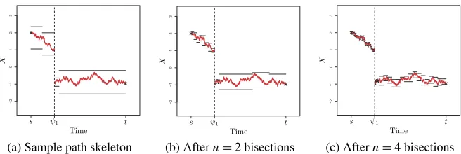
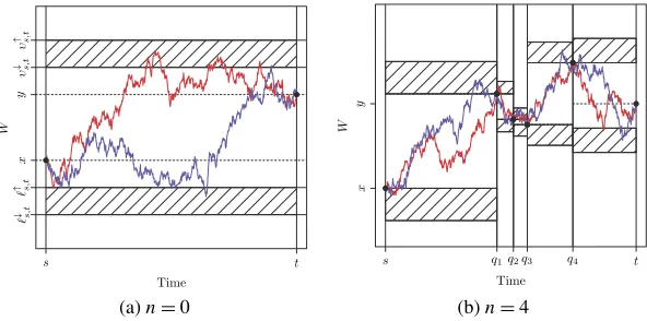
This leads to the novel AUEA detailed in Algorithm4, the recursive nature of the algorithm being illustrated in Figure4which is an extension to the example in Figure3. We outline how to simulate (unbiasedly) layer information (Step 2), intermediate skeletal points (Step 4(b)ii) and new layer information (Step 4(b)iv) in a variety of ways in Section8. Our iterative scheme outputs a skeleton comprising skeletal points and layer information for the intervals between consecutive skeletal points,
SAUEA(X):=(ξi, Xξi)κi=+01,
R[ξi−1,ξi]
X
κ+1 i=1
. (28)
The AUEA with this skeleton has the distinct advantage that Principles1,2 and3 are satis-fied directly. In particular, any finite collection of intermediate points required after the skeleton has been simulated can be simulated directly (by application of Algorithm 4 Step 4(b)ii and Step 4(b)iv), without any augmentation of the skeleton (as in Algorithm3). If necessary, further refinement of the layers given the additionally simulated points can be performed as outlined in Section8.
(a) After preliminary acceptance (Algorithm4
Step 3)
(b) After simulatingξ1(Algorithm4Step 4)
[image:19.488.248.394.56.185.2](c) After simulatingξ2 (d) After simulatingξ3
Figure 4. AUEA applied to the trajectory ofφ(X)in Figure3(whereX∼Wx,y0,T|R(X)).
required after acceptance (e.g., in the settings outlined in Sections5and9). To emphasise this, in Figure5we contrast the skeleton output from the UEA (Algorithm3, prior to augmentation) and the AUEA (Algorithm4).
In Algorithm 4, we introduce simplifying notation, motivated by the algorithm’s recursive nature in which (as shown in (26)) the acceptance probability is iteratively decomposed over intervals which have been estimated and are yet to be estimated.denotes the set comprising information required to evaluate the acceptance probability for each of the intervals still to be estimated,:= {(i)}|i=|1. Each(i)contains information regarding the time interval it applies to, the sample path at known points at either side of this interval (whichdo notnecessarily align with the end points of the sub-intervals corresponding to the remaining probabilities requiring simulation (as illustrated in Figure4)) and the associated simulated layer information, which we denote[s((i)), t ((i))],x((i)):=X←(i)−s ,y((i)):=X−→(i)
t andR (i)
(a) Example sample path skeleton output from the Unbounded Exact Algorithm (UEA; Algorithm3), SUEA(X), overlaid with two possible example sam-ple path trajectories consistent with the skeleton
[image:20.488.89.231.51.184.2](b) Example sample path skeleton output from the Adaptive Unbounded Exact Algorithm (AUEA; Al-gorithm4),SAUEA(X), overlaid with two possible example sample path trajectories consistent with the skeleton
Figure 5. Comparison of UEA and AUEA skeleton output. Hatched regions indicate layer information, whereas the asterisks indicate skeletal points.
←−s ((i))≤s((i)) < t ((i))≤ −→t ((i))). As before,R(i)
X can be used to directly compute
bounds forφfor this specific sample path over the interval[s((i)), t ((i))] (namelyL(i)X ,
UX(i)and(i)X ). We further denotem((i)):=(s((i))+t ((i)))/2,d((i)):=(t ((i))− s((i)))/2 and:=(1).
3.2.1. Implementational Considerations – Known Intermediate Points
It should be noted that if a number of intermediate points of a sample path are required and the time points at which they occur are known in advance, then rather than simulating them after the acceptance of the sample path skeleton in Algorithm4 Step 6, their simulation can be incorporated into Algorithm4. In particular, if these points are simulated immediately after Algorithm4Step 3 (this can be performed using Algorithm22as detailed in Section8.5), then we have additional layer information regarding the sample path which can be used to compute tighter bounds forφ(X[0,T])leading to a more efficient algorithm (as in Section3.2). A drawback
of this approach is that these additional points of the sample path constitute part of the resulting skeleton.
4. Exact Simulation of Jump Diffusions
following SDE,
dXt=α(Xt−)dt+dWt+dJtλ,ν, X0=x∈R, t∈ [0, T]. (29)
Denoting byQx0,T the measure induced by (29), we can draw sample paths fromQx0,T by instead drawing sample paths from an equivalent proposal measureWx0,T (a natural choice being a drift-less version of (29), which will no longer coincide with Wiener measure), and accepting them with probability proportional to the Radon–Nikodým derivative ofQx0,T with respect toWx0,T. The resulting Radon–Nikodým derivative (7) differs from that for diffusions (8) with the inclu-sion of an additional term, so the methodology of Section3can’t be applied. However, (7) can be re-expressed in a product form similar to (23) (withψ1, . . . , ψNT denoting the jump times in
the interval[0, T],ψ0:=0,ψNT+1:=T andNt:=
i≥11{ψi≤t}),
dQx0,T dWx0,T(X)=
NT+1 i=1
exp
A(Xψi−)−A(Xψi−1)−
ψi− ψi−1
φ(Xs)ds
. (30)
This form of the Radon–Nikodým derivative is the key to constructingJump Exact Algorithms (JEAs). Recall that in Section3.1.1, decomposing the Radon–Nikodým derivative for diffusions justified the simulation of sample paths by successive simulation of sample paths of shorter length over the required interval (see (23)). Similarly, jump diffusion sample paths can be simulated by simulating diffusion sample paths of shorter length between consecutive jumps.
In this section, we present three novel Jump Exact Algorithms (JEAs). In contrast with existing algorithms [13,17,20], we note that the Bounded, Unbounded and Adaptive Unbounded Exact Algorithms in Section3can all be incorporated (with an appropriate choice of layered Brownian bridge construction) within any of the JEAs we develop. In Section4.1, we present the Bounded Jump Exact Algorithm (BJEA), which is a reinterpretation and methodological extension of [13], addressing the case where there exists an explicit bound for the intensity of the jump process. In Section4.2, we present the Unbounded Jump Exact Algorithm (UJEA) which is an extension to existing exact algorithms [17,20] in which the jump intensity is only locally bounded. Finally, in Section4.3we introduce an entirely novel Adaptive Unbounded Jump Exact Algorithm (AUJEA) based on the adaptive approach of Section3.2, which should be adopted in the case where further simulation of a proposed sample path is required after acceptance.
4.1. Bounded Jump Intensity Jump Exact Algorithm
The case where the jump diffusion we want to simulate (29) has an explicit jump intensity bound (supu∈[0,T]λ(Xu)≤ <∞) is of specific interest as an especially efficient exact algorithm
can be implemented in this context. In particular, proposal jump times, 1, . . . , N T can be
simulated according to a Poisson process with the homogeneous intensityover the interval
[0, T](where NT denotes the number of events in the interval[0, T]of a Poisson process of intensity). A simple Poisson thinning argument [23] can be used to accept proposal jump times with probabilityλ(Xi)/. As noted in [13], this approach allows the construction of
Algorithm 5Bounded Jump Exact Algorithm (BJEA) [13] 1. Setj=0. Whilej< T,
(a) Simulateτ∼Exp(). Setj=j+1 andj=j−1+τ.
(b) Apply an exact algorithm to the interval[j−1, (j∧T )), obtaining skeletonSEAj .
(c) Ifj> T then setXT =XT−else,
i. With probabilityλ(Xi)/setXj:=Xj−+μj whereμj∼fν(·;Xj−), else
setXj:=Xj−.
2. ∗SimulateXrem∼N T+1 j=1 (
κj+1 i=1 W
Xξj,i−1,Xξj,i ξj,i−1,ξj,i |R
EA
X[ξj,0,ξj,κj+1]).
broken into segments corresponding precisely to the intervals between proposal jump times, then iteratively between successive times, an exact algorithm (as outlined in Section3) can be used to simulate a diffusion sample path skeleton. The terminal point of each skeleton can be used to determine whether the associated proposal jump time is accepted (and if so a jump is simulated). The Bounded Jump Exact Algorithm (BJEA) we outline in Algorithm 5 is a modification of that originally proposed in [13] (where we define0:=0, N
T+1:=T andX[s, t]to be
the trajectory ofX in the interval[s, t] ⊆ [0, T]). In particular, we simulate the proposal jump times iteratively (exploiting the exponential waiting time property of Poisson processes [23] as in Section3.2), noting that the best proposal distribution may be different for each sub-interval. Furthermore, we note that any of the exact algorithms we introduced in Section3can be incor-porated within the BJEA (and so the BJEA will satisfy at least Principles1and2). In particular, the BJEA skeleton is a concatenation of exact algorithm skeletons for the intervals between each proposal jump time, so to satisfy Principle3and simulate the sample path at further intermediate time points (Step 2), we either augment the skeleton if the exact algorithm chosen is the Un-bounded Exact Algorithm (UEA) (as discussed in Sections3.1and7), or, if the exact algorithm chosen is the Adaptive Unbounded Exact Algorithm (AUEA) then simulate them directly (as discussed in Sections3.2and8),
SBJEA(X):= N
T+1 j=1
Sj
EA(X). (31)
4.2. Unbounded Jump Intensity Jump Exact Algorithm
Considering the construction of a Jump Exact Algorithm (JEA) under the weaker Condition4
(in which we assume only that the jump intensity in (29) is locally bounded), it is not possible to first simulate the jump times as in Section 4.1. However (as in Section 3 and as noted in [17,20]), it is possible to simulate a layerR(X)∼R, and then compute a jump intensity bound
(λ≤X<∞)conditional on this layer. As such, we can construct a JEA in this case by simply
Algorithm 6Unbounded Jump Exact Algorithm (UJEA) [20] 1. Setj=0,ψj=0 andNTλ=0,
(a) Simulate skeleton end pointXT =:y∼h(y;Xψj, T −ψj).
(b) Simulate layer informationRjX[ψ
j,T]∼Rand compute j X[ψj,T].
(c) Simulate proposal jump timesNT,j∼Poi(jX[ψ
j,T](T −ψj))and j 1, . . . ,
j NT,j
iid
∼
U[ψj, T].
(d) Simulate skeleton points and diffusion at proposal jump times (X
ξ1j, . . . , Xξκj, X
1j, . . . , XN (,j ,T )j ),
i. Simulate κj ∼ Poi([UXj[ψj,T] − L j
X[ψj,T]] · (T − ψj)) and skeleton times
ξ1j, . . . , ξκj iid
∼U[ψj, T].
ii. Simulate sample path atX
ξ1j, . . . , Xξκj, X1j
, . . . , X
N (,j ,T )j ∼W x,y ψj,T|R
j X[ψj,T].
(e) With probability(1−κi=j1[(UXj[ψ
j,T]−φ(Xξij))/(U j
X[ψj,T]−L j
X[ψj,T])]), reject and
return to Step 1(a). (f) Foriin 1 toNT,j,
i. With probabilityλ(X ji)/
j
X[ψj,T]setXij−=Xij,Xij:=Xij−+μij where
μ
ji ∼fν(·;Xji),ψj+1:= j
i,j=j+1,NTλ=j, and return to Step 1(a).
2. ∗SimulateXrem∼N λ T j=0[(
κj+1 i=1 W
Xξj,i−1,Xξj,i ξj,i−1,ξj,i )|R
j X[ψj,T]].
The Unbounded Jump Exact Algorithm (UJEA) which we present in Algorithm6is a JEA construction based on the UEA and extended from [20]. The UJEA is necessarily more compli-cated than the Bounded Jump Exact Algorithm (BJEA) as simulating a layer in the UEA requires first simulating an end point. Ideally we would like to segment the interval the jump diffusion is to be simulated over into sub-intervals according to the length of time until the next jump (as in the BJEA), however, as we have simulated the end point in order to find a jump intensity bound then this is not possible. Instead we need to simulate a diffusion sample path skeleton over the entire interval (along with all proposal jump times) and then determine the time of the first ac-cepted jump (if any) and simulate it. If a jump is acac-cepted another diffusion sample path has to be proposed from the time of that jump to the end of the interval. This process is then iterated until no further jumps are accepted. The resulting UJEA satisfies Principles1and2, however, as a consequence of the layer construction, the jump diffusion skeleton is composed of theentirety of each proposed diffusion sample path skeleton. In particular, we can’t apply the strong Markov property to discard the sample path skeleton after an accepted jump because of the interaction between the layer and the sample path before and after the time of that jump.
SUJEA(X):= Nλ
T j=0
ξij, X
ξij κj+1
i=0 ,
1j, X 1j
NT,j i=1 , R
j X[ψj,T]
The UJEA doesn’t satisfy Principle3unless the skeleton is augmented (as with the UEA outlined in Sections3.1and7). As this is computationally expensive, it is not recommended in practice. Alternatively we could use the AUEA within the UJEA to directly satisfy Principle3, however it is more efficient in this case to implement the Adaptive Unbounded Jump Exact Algorithm (AUJEA) which will be described in Section4.3(for the same reasons in which the AUEA is more efficient than the UEA, as detailed in Section3.2).
4.3. Adaptive Unbounded Jump Intensity Jump Exact Algorithm
The novel Adaptive Unbounded Jump Exact Algorithm (AUJEA) which we present in Algo-rithm7 is based on the Adaptive Unbounded Exact Algorithm (AUEA) and a reinterpretation of the Unbounded Jump Exact Algorithm (UJEA). Considering the UJEA, note that if we sim-ulate diffusion sample path skeletons using the AUEA then, as the AUEA satisfies Principle3
directly, we can simulate proposal jump times after proposing and accepting a diffusion sam-ple path as opposed to simulating the proposal times in conjunction with the samsam-ple path (see Algorithm 6Step 1(d)ii). As such, we only need to simulate the next proposal jump time (as opposed to all of the jump times), which (as argued in Section3.2), provides further information about the sample path. In particular, the proposal jump time necessarily lies between two existing
Algorithm 7Adaptive Unbounded Jump Exact Algorithm (AUJEA) 1. Setj=0 andψj=0.
2. Apply AUEA to interval[ψj, T], obtaining skeletonS[ ψj,T] AUEA.
3. Setk=0 andkj=ψj. Whilekj< T,
(a) Computej X[kj,T].
(b) Simulateτ∼Exp(j
X[kj,T]). Setk=k+1 and j k =
j k−1+τ.
(c) Ifkj≤T,
i. SimulateX jk ∼W
Xψj,XT ψj,T |S
[ψj,T] AUEA.
ii. Simulate R[ξ j
−,kj]
X and R
[kj,ξ+]
X and set S
[ψj,T] AUEA :=S
[ψj,T]
AUEA ∪ {Xkj, R
[ξ−j,kj]
X ,
R[ j k,ξ+] X } \R
[ξ−j,ξ+]
X .
iii. With probability λ(X kj)/
j
X[kj−1,T] set Xkj− = X
jk, Xkj :=Xjk−+μkj
where μ
kj ∼fν(·;Xjk), ψj+1:= j
k, retain S
[ψj,ψj+1)
AUEA , discard S [ψj+1,T]
AUEA , set j =j+1 and return to Step 2.
4. Let skeletal points χ1, . . . , χm denote the order statistics of the time points in SAUJEA:= j+1
i=1S [ψi−1,ψi)
AUEA .
5. ∗SimulateXrem∼im=+11W[Xχi−1,Xχi) [χi−1,χi) |R
[χi−1,χi)

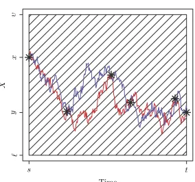
![Figure 8. Example sample path trajectories W ∼ Wx,ys,t |(W(s,t) ∈ [ℓ,υ]).](https://thumb-us.123doks.com/thumbv2/123dok_us/9510472.456432/33.488.146.314.52.209/figure-example-sample-path-trajectories-w-wx.webp)
![Figure 9. Example sample path trajectories W ∼ Wx,ys,t |( ˆm ∈ [ℓ↓,ℓ↑], ˇm ∈ [υ↓,υ↑],q1:n,W).](https://thumb-us.123doks.com/thumbv2/123dok_us/9510472.456432/36.488.107.405.53.201/figure-example-sample-path-trajectories-m.webp)
![Figure 11. Density of intersection layer intermediate point overlaid with piecewise constant bound calcu-lated using a mesh of size 20 over the interval [ℓ↓,υ↑] and the corresponding local Lipschitz constants.](https://thumb-us.123doks.com/thumbv2/123dok_us/9510472.456432/50.488.173.341.53.209/intersection-intermediate-overlaid-piecewise-interval-corresponding-lipschitz-constants.webp)
