A method for normal-mode-based model reduction in nonlinear
dynamics of slender structures
Yinan Wang, Rafael Palacios
⇑, Andrew Wynn
Department of Aeronautics, Imperial College, London SW7 2AZ, United Kingdom
a r t i c l e
i n f o
Article history: Received 2 April 2015 Accepted 7 July 2015 Available online 28 July 2015
Keywords: Model reduction
Geometrically-nonlinear structures Static condensation
Nonlinear vibrations Modal analysis
a b s t r a c t
This paper introduces a nonlinear reduced-order modelling methodology for finite-element models of structures with slender subcomponents and inertia represented by lumped masses along main load paths. The constructed models have dynamics described by 1-D intrinsic equations of motion, which are further written in modal co-ordinates. This yields finite-dimensional approximations of the system dynamics with only quadratic nonlinearities. Evaluation of the problem coefficients is performed from static condensation of the original model on the lumped masses. The method exploits the multi-point constraints typically used to obtain sectional loads in aircraft aeroelastic analysis. The technique is illustrated on simple 3D structural models built using solid elements.
Ó2015 The Authors. Published by Elsevier Ltd. This is an open access article under the CC BY license (http:// creativecommons.org/licenses/by/4.0/).
1. Introduction
The dynamic aeroelastic response of most existing air vehicles and wind turbines is characterised by small-amplitude elastic dis-placements at relatively low frequencies. As a result, their struc-tural description for aeromechanic studies has long been based on linear theories and solutions have been sought using linear nor-mal modes (LNMs) of the structure in vacuum. This also has the additional advantage that the time-domain aerodynamics can be obtained for wall disturbances defined by that relatively small number of LNMs. The demand for ever higher design efficiency, however, is leading to much more flexible high-aspect-ratio light-weight wings and blades with major implications for the require-ments of computational tools[1]: First, the low-frequency elastic response is dynamically coupled with the rigid-body dynamics of the vehicle; second, geometrically-nonlinear effects may be signif-icant in the structural response; and finally, full coupling is required with the fluid solver at simulation time. Consequently, the resulting computational cost is increased manifold[2,3] and may become prohibitive for routine design analysis. An additional requirement is posed by the initial (model-based) design of the flight control and gust/manoeuvre load alleviation systems, which call for the ability to generate small-size descriptions of the system dynamics using methods of model reduction[4].
While model reduction of linear systems is very well developed, dimensional reduction of general nonlinear systems heavily depends on the characteristics of the relevant nonlinear phenom-ena and the structure of their representation. Parametrised modal projections have been shown for flexible bodies with arbitrary rigid-body kinematics and small elastic displacements[5,6] and have also been extended to the case of aeroelastic systems mod-elling flexible manoeuvring aircraft[7,8]. For nonlinear vibrations, normal form theory allows dimensional reduction of the free response in the structure’s Nonlinear Normal Modes (NNMs) [9,10]. NNMs provide a fundamental understanding of the system dynamic characteristics, but they do not define, unlike LNMs, a basis for projection of the forced response of the geometrically-nonlinear structure. Instead, the LNMs themselves (either on undeformed or deformed equilibrium conditions) are commonly employed as a basis for projection in nonlinear vibra-tions[11,12], although methods based on system responses to pre-scribed forces, such as proper orthogonal decomposition or centroidal Voronoi tessellation [13], have also been proposed. The main limitation of those methods comes from the fact that in solutions based on approximations of the displacement field, one needs to retain cubic terms to capture softening/hardening effects on the stiffness. The corresponding fourth-order tensors are, in general, fully populated, as the banded structure in the finite-element discretisation disappears in the global basis. As a result, the computational cost grows very quickly with the number of LNMs.
Thus, the common approach has been to use structural slenderness to construct purpose-built models based on
http://dx.doi.org/10.1016/j.compstruc.2015.07.001 0045-7949/Ó2015 The Authors. Published by Elsevier Ltd.
This is an open access article under the CC BY license (http://creativecommons.org/licenses/by/4.0/). ⇑Corresponding author at: Room 355, Roderic Hill Building, Imperial College,
South Kensington Campus, London SW7 2AZ, United Kingdom. Tel.: +44 (0)20 7594 5075.
E-mail address:[email protected](R. Palacios).
Contents lists available atScienceDirect
Computers and Structures
geometrically-nonlinear beam elements[14–17]. The constitutive relations (i.e., the matrices of mass and stiffness per unit length) are based on either estimates of section moments of inertia or purpose-built homogenisation tools based on either cross-sectional[18]or unit-cell[19]analysis. This results in a mod-erate simulation effort for configuration studies, as well as proce-dures to synthesise control systems from local linearisation around nonlinear static equilibria[20,21]. While this has provided substantial insight into the nonlinear response of highly-flexible aircraft and wind turbines, none of these procedures currently relate to the actual, detailed and typically very large (with the number of degrees of freedom typically measured in millions) 3-D finite-element (FEM) models, which are built, validated, and refined, in the various loops of the design cycle. These models col-lect the engineering knowledge of an organisation and should be the basis for any numerical analysis aimed at structural certification.
Since the low-frequency dynamic response of slender structures is strongly dominated by its lengthwise deformations, it is still interesting to establish reduction methods from those large 3-D models into much more compact 1-D representations. The typical approach is to construct 1D models with a distribution of mass and stiffness that matches section-averaged responses to unit sta-tic loads and/or a number of LNMs[22]. The main drawback of this approach is that, to obtain an accurate representation of the origi-nal model, one needs to identify a large number of coefficients on that approximate beam discretization (in general, 21 independent coefficients in the sectional mass and stiffness matrix of each beam element). Typically the identification is only carried out on a very small number of modes, which does not guarantee modelling accuracy in nonlinear problems. To overcome this, this paper will present a hybrid approach that combines the model fidelity encap-sulated in the LNMs of the large 3-D model with the efficiency of 1-D models to capture the dominant geometrically-nonlinear effects in slender structures. This is achieved by introducing the dimensional reduction on the linear eigenvalue analysis in the 3-D FEM model, by means of static or dynamic condensation onto nodes located along the main load path. In parallel to this, the geometrically-nonlinear beam equations are projected into the basis defined by its LNMs. Finally, the mode shapes in the condensed 3-D model are treated as 1-D functions of the arc length along the reference line and thus used in the modal beam equations. As it will be shown, this can be done solely by post-processing information obtained from the 3-D model, i.e.,
without explicitly constructing a beam finite-element model. The result is a formulation that (1) characterises the nonlinear vibra-tions in modal space; and (2) uses the mode shapes and frequen-cies corresponding to the 3-D FEM.
The first step is to identify a suitable nonlinear beam theory. Among the many solutions in the literature, intrinsic descriptions [23–25]will be particularly useful here. An intrinsic beam theory draws upon Kirchhoff’s analogy between the spatial and time derivatives [26]to define a two-field Hamiltonian description of the beam dynamics in first-derivatives, i.e., strains and velocities. This results in a formulation that closely resembles that of rigid-body dynamics, with first-order equations of motion in both beam strains and velocities and, critically for this work, quadratic nonlinearities on those primary states. As in rigid-body dynamics, the solution process is closed by the propagation equations to obtain load displacements and rotations. The infinite-degree non-linearities associated with the finite rotations are then transferred to that post-processing step. Previous work by the authors[27]has identified energy-preserving conditions in both the infinite-dimensional and the truncated modal finite-infinite-dimensional system equation, due to the symmetries present in the reduced modal description. Following on from that work, this paper will investi-gate the generation of the equations of motion in intrinsic modal coordinates from built-up 3-D FEM models.
The starting point is the assumption that such a 3-D model of the structure already exists for linear vibration analysis. This FEM model is then reduced using Guyan’s method [28] to a small set of grid points along the main load paths. The selection of those condensation points is therefore critical, but it can be performed with similar criteria to those used in the selection of monitoring stations for aircraft dynamic loads analysis [29]. It will be assumed that the model mass is lumped on those nodes, which reflects a typical situation in full-aircraft models for vibration analysis. More sophisticated methods of dynamic condensation are available in the literature [30,31] and they could be also considered within the approach proposed in this paper. However, Guyan reduction is arguably the most common condensation method in aerospace applications and is readily available in most finite-element packages, so it is therefore pre-ferred here. The LNMs of the full 3-D model on the set of beam nodes will then be used to define directly the different coeffi-cients of the intrinsic equations in modal coordinates. This pro-cedure will be illustrated in the final section of the paper with two numerical examples.
Nomenclature
CðsÞ cross-sectional compliance matrix
fðs;tÞ beam internal forces in material coordinates f1ðs;tÞ applied forces/moments per unit beam length
kðs;tÞ beam curvatures in material coordinates k0ðsÞ initial beam curvatures in material coordinates
Ka stiffness matrix in reduced set of 3-D FEM problem mðs;tÞ beam internal moments in material coordinates Ma mass matrix in reduced set of 3-D FEM problem MðsÞ cross-sectional mass matrix
pðs;tÞ beam local position vector
qðtÞ intrinsic modal coordinates (all components) q1ðtÞ intrinsic modal coordinates (velocity component)
q2ðtÞ intrinsic modal coordinates (stress resultant
compo-nent)
Rðs;tÞ beam local coordinate transformation matrix s curvilinear coordinate along main load path t time
uðs;tÞ beam local displacements in material coordinates
v
ðs;tÞ beam translational velocities in material coordinates W skew-symmetric matrix with natural frequencies x1ðs;tÞ local translational/angular velocity state vectorx2ðs;tÞ internal force/moment state vector
U0jðsÞ natural mode shapejin global displacements U1jðsÞ natural mode shapejin intrinsic velocities U2jðsÞ natural mode shapejin intrinsic sectionalforces Uaj discrete mode shapejin reduced set of 3-D FEM
prob-lem
X diagonal matrix with natural frequencies
x
jx
ðs;tÞ beam angular velocities in material coordinatesx
C cutoff angular frequencyx
j natural angular frequency of modejf0ðs;tÞ scalar part of quaternion
2. 1-D geometrically-nonlinear description in modal coordinates
We will first describe the intrinsic equations of motion for a geometrically-nonlinear composite beam, since this formulation is the basis of the model reduction method used in this work. Only the main results are presented here, and the reader is referred for additional details to the original paper by Hodges[23]. This will then be followed by a projection of the equations into a modal space, as it was performed by Palacios[32]. Finally, the intrinsic variables are expressed in terms of local displacements and rota-tions to link the results to those obtained from the condensation of a general 3-D FEM model of the structure in Section3.
2.1. Intrinsic beam equations
A beam will be defined as the solid determined by the rigid motion of cross sections linked to a deformable space curve, C
(Cosserat’s model). There are no assumptions on the sectional material or geometric properties, other than the condition of slen-derness. Letsbe the arc length,
v
ðs;tÞandx
ðs;tÞthe instantaneous translational and angular inertial velocities, andfðs;tÞandmðs;tÞthe sectional internal forces and moments (stress resultants) along the reference line. Vectors are expressed in their components in the instantaneous local (deformed) material frame. Using these magnitudes and using dots and primes to refer to their derivatives with time,t, and the arc length,s, respectively, Hodges[23]has derived the intrinsic form of the beam equations of motion, which are written here as[32]
Mx_1x02Ex2þ L1ðx1ÞMx1þ L2ðx2ÞCx2¼f1;
Cx_2x01þE
>x
1 L>1ðx1ÞCx2¼0:
ð1Þ
The state vectorsx1andx2are defined as
x1:¼
v
x
; x2:¼
f m
: ð2Þ
The forcing term is the vectorf1ðs;tÞ, which includes the applied
forces and moments per unit length, also written in their compo-nents in the instantaneous material frame. Thus a constant value off1corresponds to follower forces.MðsÞandCðsÞare the sectional
mass and compliance matrices, respectively, which are 66 sym-metric matrices. Finally, the matrixEand linear matrix operators
L1andL2are
E:¼ k~0 0 ~ e1 k~0
" #
; L1ðx1Þ:¼
~
x
0~
v
x
~
; and L2ðx2Þ:¼ 0
~ f ~f m~
" #
; ð3Þ
where~is the skew-symmetric (or cross-product) operator,k0ðsÞis
the initial pretwist and curvature of the reference line, and e1:¼½1;0;0is the unit vector. Eqs.(1)are solved with the
corre-sponding boundary and initial conditions, which are also written in terms of velocities and forces[23].
The formulation being presented here is completely equivalent to a standard displacement-based nonlinear composite beam for-mulation, but without including displacements and rotations as primary variables. In the intrinsic description, displacements and rotations are dependent variables that only appear explicitly in Eq. (1)when applied forces and moments, f1, depend on them.
Local values of the displacement and rotations are obtained either from time integration of the inertial velocities, as in rigid-body dynamics; or from spatial integration of the strains corresponding to the stress resultants, as with the Frenet–Serret formulae in dif-ferential geometry. The first approach will be followed here, fol-lowing Ref. [32]. If the local orientation with respect to a
reference inertial frame is defined by quaternions,ðf0ðs;tÞ;fðs;tÞÞ,
they satisfy
_
f0¼
1 2
x
>f;
_
f¼1
2ðf0
x
x
~fÞ:ð4Þ
The position vectorrðs;tÞalong the beam with respect to the same inertial reference frame (and given in its components in that frame) is finally obtained from time integration of the local inertial velocity, as
_
r¼Rv; ð5Þ
with Rðs;tÞ the local rotation matrix corresponding to the quaternions obtained in Eq.(4), which can be written as
R¼ f f01þ~f
f f01~f
>
; ð6Þ
where1is the identity matrix.
2.2. Nonlinear large-displacement equations in modal coordinates
The LNMs of the structure in intrinsic variables are obtained from the linearisation of Eq.(1)around the unloaded conditions. For small values ofDx1andDx2,
M
D
x_1D
x02E
D
x2¼D
f1;C
D
x_2D
x01þE
>
D
x1¼0:ð7Þ
Non-trivial solutions forDf1¼0are of the form1
D
x1ðs;tÞ ¼U1jðsÞsinðx
jtÞ;D
x2ðs;tÞ ¼U2jðsÞcosðx
jtÞ;ð8Þ
where U1jðsÞ and U2jðsÞ are the mode shapes in sectional
lin-ear/angular velocity and stress resultant variables respectively. The modesU1j andU2j are therefore solutions to the eigenvalue
equation
E>@
@s
x
jCðsÞx
jMðsÞ E@@s" #
U1jðsÞ
U2jðsÞ
¼0: ð9Þ
Wynn et al.[27]have shown, using the structure of the nonlinear intrinsic Eq.(1), that this set of modes is always space-spanning. In general, the solution to Eq.(8)can only be obtained numerically. The normalisation in Eq.(8)is chosen such that
hU1j;MU1ki ¼djk; hU2j;CU2ki ¼djk;
ð10Þ
wherehg;hi:¼RCg>hdsis the inner product in the 1-D domain, defined on any pair of functionsgðsÞandhðsÞ. Using Einstein nota-tion to sum over repeated indices, the modal projecnota-tion of the state vectors is now defined as
x1ðs;tÞ ¼U1jðsÞq1jðtÞ;
x2ðs;tÞ ¼U2jðsÞq2jðtÞ;
ð11Þ
whereq1jandq2jare pairs ofintrinsic modal coordinates. Note that,
since this is a first-order theory, each LNM is associated to two gen-eralised coordinates that effectively corresponds to the real and imaginary components of a complex modal amplitude. After substi-tuting Eq.(11)into(1)and enforcing the orthogonality conditions (10), the finite-dimensional equations of motion in intrinsic modal
1The general solution to this first-order system would be of the formU
jexjtwithUj
being a complex variable. It is easy to see that the eigenvectors have the structure
Uj¼ i
U1j
U2j
and this is implicitly used here to define only real modes and
coordinates are written as[32]
_
q¼WqþNðqÞqþ
g
; ð12Þwith
q¼ q1 q2
;
g
¼g
10
; ð13Þ
and the following coefficients for the linear and quadratic terms,
W:¼ 0 X
X 0
and NðqÞ:¼ q1‘C ‘
1 q2‘C ‘
2
q2‘ðC ‘
2Þ
> 0
" #
: ð14Þ
Here, we have definedX:¼diagð
x
1;. . .;x
NÞ;g
1jðtÞ:¼ hU1j;f1i, andðC‘1Þjk:¼ hU1j;L1ðU1kÞMU1‘i;
ðC‘
2Þjk:¼ hU1j;L2ðU2kÞCU2‘i:
ð15Þ
The coefficients of the quadratic terms in the equation,C, which are responsible for the modal couplings in the system dynamics, are obtained from integral equations involving the mode shapes and the mass and compliance matrices, Eq.(15). The constant coeffi-cientsW;C1 and C2, together with the mode shapes of Eq. (11),
are the only information required to construct a geometrically-nonlinear description in intrinsic modal coordinates. As we will show below, that information can be directly extracted from a built-up 3-D FEM model of the actual configuration. In Ref.[27], we have discussed the Hamiltonian structure of Eq.(12)and also described the energy-preserving properties of the system. It was shown that the finite-dimensional approximation of Eq.(12) con-serves total system energy. Total system momentum is however not necessarily conserved and it needs to be enforced via conver-gence in the solution. This will be exemplified in the results section.
2.3. Spatial interpolation scheme in the lumped-mass problem
The nonlinear coupling coefficients in(15)are computed from integrals of the intrinsic modes along the reference line. If the modal values of the intrinsic variablex1andx2 are only known
at discrete points (as would be the case during the condensation process described later), we would need to define an interpolation scheme to interpolate these variable to compute the coupling coef-ficients. Thus we now seek a suitable spatial interpolation of the modes in primary intrinsic variables (local velocities and sectional force resultants) along the reference line from the mode shapes obtained at discrete points (analysis nodes). Note that we are not trying to defineshape functionsfor a finite-element discretisation and the interpolation will be for the sole purpose of computing the nonlinear system, with the linear modes that are assumed to be already known at discrete analysis nodes from a previous anal-ysis. A low-order interpolation scheme is sought and, if required, the number of nodes can be increased to reduce the errors associ-ated with the low-order scheme. Although higher-order schemes are entirely possible, we will demonstrate in Section5.2that the current scheme is sufficient to achieve convergence without requiring an excessively large number of nodes.
First, we define the variablex0as a six-element vector
contain-ing the linear rotation and displacement degrees of freedoms at each point. As the discrete solution provides exact displacement and velocity information on the set of analysis nodes, we will regard the values of x0 and x1 of the continuous solution to be
exactly equal to the discrete solution at the reference points. We then note that displacements and velocities on the structure must be continuous, thus in the lowest-order scheme we regardx0and
x1to vary linearly on each reference line segment between two
adjacent reference nodes, on which the values are known exactly.
If we definex1;ias the discretised value ofx1defined at nodei, that
is,x1;i¼x1ðsiÞ, linear interpolation results in
x1ffi
X
i
u
1;ix1;i; ð16Þwith
u
1;iðsÞ ¼ ssi1sisi1 si1<s<si ssiþ1
sisiþ1 si<s<siþ1
0 otherwise
8 > < >
: : ð17Þ
This is similarly carried out onx0. As the sectional forces are not
required to be continuous, we subsequently regard x2 as being
piecewise-constant along the reference line, which can be repre-sented as
x2ffi
X
i
u
2;iþ12x2;iþ
1
2 ð18Þ
withx2;iþ1
2the stress resultant at the midpoint of the reference line
segment and
u
2;iþ12ðsÞ ¼
1 si<s<siþ1
0 otherwise
ð19Þ
This thus defines the interpolated intrinsic statesx1andx2at every
pointsalong the reference line from the discretised intrinsic vari-ablesx1;i andx2;iþ1
2. Similarly, the intrinsic modesU1ðsÞandU2ðsÞ
will also follow this interpolation scheme. In the next section we will make use of these interpolations when computing the nonlinear coupling coefficients in the modal system.
3. Static condensation of the linear 3-D lumped-mass problem and identification of nonlinear modal coefficients
As outlined in the introduction, we seek to utilise a linear 3D FE model of the slender structure to obtain the coefficients in(12). This will be achieved by the application of Guyan condensation to reduce the linear equations of motion of the 3D model onto the degrees of freedom of a small set of analysis nodes. The starting point of the analysis in this section is a linear 3D FE model of the structure with nodal displacement, and possibly rotations, as the degrees of freedom, on which we define a set of analysis degrees of freedom. The natural modes are then obtained on this reduced set. Here the error can become significant at the higher frequencies [33]or with a poor selection of the analysis degrees of freedom[34]. For very large systems, the matrix inversion itself can also be replaced by a Gauss–Jordan elimination[35]or any other suitable procedure. In this work however, we first lump the structural iner-tia of the full 3D model onto the set ofNaanalysis nodes, and then
we obtain the mass and stiffness matrices that describe the linear dynamics of this reduced set of degrees of freedom. We should note that this lumping of masses, which used in a number of finite-element descriptions [36], is common practice in full aircraft vibration analysis. The relation between the 3D model and the set of analysis nodes can be seen inFig. 1. We define the six-state (three in displacement and three in rotation) vector variablexa;i2R6to
describe the (linear) nodal displacement and rotation at thei-th condensation node (with i¼1;. . .;Na). The corresponding linear
normal modes,Uaj2R6Na, of the reduced system are then obtained
from
x
2jMaUajþKaUaj¼0 ð20Þ
whereMais block diagonal and contains the mass matrices of
indi-vidual lumped-mass nodes ML2R66, and Ka is, in general, fully
considers linear analysis only, thus theDsign is dropped from all variables, which are assumed to be small.
The reduced system(20)is discrete in space with displacements and velocities defined only at theNalumped mass nodes. For
non-linear analysis using the intrinsic modal description, we consider reference lines that connect the analysis nodes along the load paths of the structure as shown inFig. 1, and then seek a continu-ous description of the variables along the reference lines. The linear normal modes on the continuous problem will be obtained from the discrete system in (20) and will be used to compute the geometrically-nonlinear dynamics of the structure using the intrinsic modal formulation.
3.1. Computation of intrinsic modes from condensation
We will identify next the relation that links the (discrete) linear normal modes defined by(20),Uaj, to the (continuous) intrinsic
modesU1jðsÞandU2jðsÞ. Since the linear intrinsic description and
the displacement-based description are different formulations of the same (linear) problem, the eigenvalues and eigenvectors of the two formulations are enforced to match exactly. This will then provide the process by which the intrinsic modes of the continu-ous, 1D problem, and thus the nonlinear modal system(12), can be computed from the 3D FE model.
3.1.1. Velocity modes
As the intrinsic variables (velocityx1and sectional forcex2) are
defined using the local frame at each point of the reference line
whereas the displacement and rotation x0 is not necessarily
defined in the same frame, we will first define the transformation from the frame used byx0ðs;tÞinto the local frame used by
intrin-sic variablesx1ðs;tÞas
x1ðs;tÞ ¼TðsÞx_0ðs;tÞ; ð21Þ
similar to(5).TðsÞis a 66 matrix. In the particular case that both the displacement and rotation components inx0are defined in the
global inertial frame,TðsÞwill take the form of
TðsÞ ¼ RðsÞ 1
0 0 RðsÞ1
" #
ð22Þ
whereRðsÞfrom(5)is taken at the unloaded configuration. Using (21) and (8), we write the eigenvalue solution to the structural problem as
x1ðs;tÞ ¼TðsÞx_0jðs;tÞ ¼U1jðsÞsinð
x
jtÞ ð23ÞTherefore, the eigenvalue solution inx0 that corresponds to the
above solution inx1will be
x0ðs;tÞ ¼
1
x
jTðsÞ1U1jðsÞcosð
x
jtÞ ð24ÞWe now define the linear normal mode shapes in displacements and rotations along every point on the reference line asU0j, with
corresponding natural angular frequencies
x
j, as taking the form of [image:5.595.138.451.70.440.2]x0ðs;tÞ ¼ cosð
x
jtÞU0jðsÞ: ð25Þwherex0is the eigenvalue solution to the structural equations cast
inx0in a displacement-based formulation, which will not be
repro-duced here.
From(21) and (25), a definition of the continuous displacement and rotation modes in terms of intrinsic velocity variables, with the correct sign, is
U1jðsÞ ¼
x
jTðsÞU0jðsÞ; ð26ÞFinally, we obtain the linear normal modes in displacements and rotations for the discrete, reduced problem(20)asUaj, with
corre-sponding natural angular frequencies
x
j, fromx
2 jMaþKa
Uaj¼0: ð27Þ
Consistent with the interpolation scheme used in this work described in Section 2.3, we now regard each continuous displacement-rotation mode shapeU0jat each analysis node as
U0jðsiÞ ¼Uaj;i; i¼1;. . .;Na: ð28Þ
Therefore, relations (28) and (26) allow us to relate the natural modes of the continuous, 1D problem to the natural modes of the discrete, reduced FE system and computeU1j from the knowledge
ofUaj.
The momentum modeMU1jis obtained by simply multiplying
the nodal lumped massML;iwith the nodal values of the velocity
modeU1jðsiÞ. The reference frame ofMU1jðsiÞcan be the local
ref-erence frames of any refref-erence line segment connecting to it as this is only used to compute the coupling coefficientC1in(12).
3.1.2. Force modes
We have outlined the process of obtainingU1jof the continuous
1D problem fromUajof the discrete, reduced structure in the
pre-vious section. We will now proceed to describe how the informa-tion from Uaj is independently used to construct the intrinsic
mode shape in sectional forcesU2jin the 1D problem. In particular,
we seek to obtain the modes in sectional force,U2j, and the
corre-sponding modes in sectional strainsCU2jdirectly fromUajand the
stiffness matrixKa in Eq.(20) without explicitly computing the
sectional stiffness C, which is in general, a function of the arc length s. For clarity we shall use CU2j to indicate the
directly-computed sectional strain modes to emphasise the fact thatCis not explicitly known.
We first compute the intrinsic mode in sectional strains,CU2j
from the corresponding intrinsic mode in velocityU1j, by applying
the linearised intrinsic equations. From the second equation in(7) we obtain,
x
jCU2jðsÞ ¼ U01jðsÞ þE >U1jðsÞ: ð29Þ
Using the linear interpolation inU1jin Eq.(16)and piecewise
con-stantCU2jin Eq.(18), we can also write in discrete form as
CU2j;iþ1
2¼
x
1
j
U1j;iþ1U1j;i
siþ1si
þE>U1j;iþU1j;iþ1
2
; ð30Þ
The sectional force modesU2jwill also be computeddirectlyfrom
Uaj, i.e., there is no need for explicit knowledge of the sectional
compliance matrixCin this method. Similar toCU2j, we can rewrite
the first equation in(7)and obtain
U02jðsÞ þEU2jðsÞ ¼
x
jMU1jðsÞ ð31Þthat describes the relation between a pair ofU2j andU1jwith the
correct sign. However for a lumped-mass model whereMis concen-trated at the nodes, this equation encounters issues with geometry and is difficult to apply directly. In order to clarify the method used in our approach, we seek an alternative, integral description toU2j.
We first note that the termKaxain(20)describes the elastic forces
fKand momentsmKexperienced on each of the 6Nadegrees of
free-dom on the analysis nodes of the system (3 displacement and 3 rotation variables in each node) caused by the distribution of dis-placements/rotationsxa. Thus at each nodei,
fK;i
mK;i
¼ ðKaxaÞji: ð32Þ
We also note that, in the linear case, this elastic force can equally be described by an imbalance of sectional (internal) forces, i.e., there is a one-to-one relation between the distribution ofx2and the
distri-bution offKandmK (thusxa). In order to obtain the relation, we
consider the linear static problem where the structure experiences an internal stress distributionx2which arises from the application
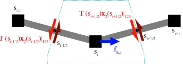
of fK andmK. We observe that for node i inFig. 2, the relation
between the forces described by theKa matrix, and internal
sec-tional forces (which we always evaluate at the midpoint of the ref-erence line segments), is
fK;i
mK;i
¼ ðTiþ1
2þ L1ð
q
iþ12q
iÞÞx2;iþ1
2 ðTi
1
2þ L1ð
q
i12q
iÞÞx2;i1 2
ð33Þ
where
q
i¼ri
0
ð34Þ
Due to the piecewise-constant interpolation ofx2within each
seg-ment, we evaluate the value ofx2(andU2j) at the midpoint of each
segment, i.e.,siþ1
2andsi12. The sign in front of each sectional force
term is dependent on the direction of increasings, as reversing this direction reverses the definition of sectional force and thus reverses the sign.
Using these definitions, we could write the relation betweenUaj
andU2jat nodesiusing(33). This equation can be easily extended
to nodes that contain multiple connectivity. Inverting these equa-tions allows us to obtainU2jfromUajand
x
j, by starting from anyunconstrained end point on the assembly (where the sectional forces and moments are zero by definition), then computingU2j
at each subsequent segment from the value ofU2jat the previous
segment andKaUajat the node. For example, for a single, straight
beam without any branching structures, the method can be written as
U2jðsiþ1
2Þ ¼
X
k>i
ðKaUaÞjk;123
X
k>i
ðKaUaÞjk;456þ ð~rk~riþ1
2ÞðKaUaÞjk;123
0 B B @
1 C C
A: ð35Þ
From this complete knowledge ofU1;U2;MU1andCU2(asCU2), we
can compute all the coefficients(15)in the equations of motion in intrinsic modal coordinates(12).
To summarise, the condensation method described in this work is carried out in the four steps summarised inFig. 1, namely:
Step I, the starting point is a 3D FE model of the structure with the requirement that inertia is lumped onto a set of analysis nodes along load paths.
Step II, we carry out the Guyan reduction on the 3D model, arriving at the reduced mass and stiffness matrices describing the linear dynamics of the discrete reduced degrees of freedom in displacement and rotations xa and a linear system described
by(20).
Step III, the natural modes described in discrete global displace-ments and rotations of the analysis nodesUaare obtained from the
Step IV, we obtain the equivalent, continuous intrinsic modes U1;U2;MU1andCU2from the discrete natural modesUa.
The nonlinear intrinsic modal system(12)is obtained by com-puting the coupling coefficients from the continuous intrinsic modes. Thus, we have developed a method of arriving at a geomet-rically nonlinear, modal description of a slender structure from a linear 3D FE model of the structure.
4. Numerical aspects of the implementation
4.1. Time-marching schemes
The problem has been cast as a first-order nonlinear ODE and will be marched using the explicit 4th-order Runge–Kutta numer-ical scheme. The largest permissible time-step for stable time marching of the system (Eq.(12)) is determined by the inverse of the largest eigenvalue in theWmatrix. As modes of increasing fre-quency are included for better accuracy of results, the permissible time-step becomes smaller, i.e., the problem becomes increasingly stiff in the numerical sense.
This problem can be mitigated by using the structure of the nonlinear modal equations. Higher modes are required to capture the highly deformed shapes, but the fast dynamics of the associ-ated natural frequencies (the linear part of Eq. (12)) are not of interest. Here we define a mode as being high-frequency when its associated eigenvalue,
x
j, is higher than a specified cut-offfre-quency,
x
C. Otherwise it is regarded as being low-frequency. Wenow split q into two parts containing the low- and high-frequency modes, qL and qH, respectively, that is,
q¼ q>
L q>H
>
. Using this, Eq.(12)can be split into
_
qL¼WLqLþNLðqÞqþ
g
L; _qH¼WHqHþNHðqÞqþ
g
Hð36Þ
Under a slow external forcing, the linear part of the second equa-tion, which defines a set of high-frequency harmonic oscillators, operates at a very different frequency to the quadratic part of the equation, which contains contributions from geometrically nonlin-ear couplings, and to the external forcing, whose characteristic fre-quency can be orders of magnitudes lower than the linear part. Therefore, if only the low-frequency dynamics are of interest, the system can be approximated by regarding a time-averagedqHthat
reacts instantaneously to excitations from NHðqÞq and
g
H terms.This approximation effectively removes the high-frequency dynam-ics fromqHstates and converts Eq.(36)into a set of
differential–al-gebraic equations (DAE),
_
qL¼WLqLþNLðqÞqþ
g
L;qH¼ W1
H ðNHðqÞqþ
g
HÞ;ð37Þ
withq¼ q>
L q>H
>
. This set of equations is marched here by first iterating the value ofqHusing the currently known values of system
statesqLwith the second equation of Eq.(37), then computing the
value ofq_Lusing the first equation to advance the time marching.
Results using this method will be shown in Section5and will be compared to full simulation of Eq.(12).
4.2. Time and memory requirements
The computational complexity of marching the solution at every timestep is dominated by the computation of the quadratic coupling termsNðqÞq in Eq. (12). As the coupling is quadratic, the total number of multiplications required will increase with the number of modes retained asOðN3MÞ. The memory required also
scales withOðN3
MÞ, with each of the two sets of (fully-populated)C
coefficients requiring 8N3Mbytes of memory. The timestep itself can
be adjusted using the method described above.
TheOðN3MÞtime and memory complexity arises from the global
nature of the coupling, which is non-zero between each pair of nat-ural modes. However we observe that each beam segment only couples locally and it can be shown easily that a decomposition ofC‘
1¼B
1
1 D
‘
1B1is possible, where columnjof the constant matrix
B1 contain the vectorised form ofU1j. Under this decomposition,
eachD‘
1matrix will be a banded diagonal matrix with a very low
bandwidth and contains OðNMÞ non-zero elements. A similar decomposition is possible for C‘
2 which reduces the total time
and memory requirement toOðN2 MÞ.
5. Numerical examples
Two numerical examples will be used to demonstrate the pre-sent methodology. The first is a simple cantilever box-beam config-uration, for which analytical solutions are available. This will allow verification of the various steps in the analysis. Next, an application of the methodology developed in this paper will be performed on a more complex unsupported structure under large rigid body motions and elastic deformations.
5.1. Thin-walled prismatic isotropic cantilever
Consider a simple prismatic thin-walled cantilever structure with constant dimensionless properties (E¼106;
m
[image:7.595.145.445.68.173.2]¼0:3;
q
¼1) and a rectangular cross section. The box beam has lengthL¼20, widthw¼1, heighth¼0:1, and walls of thicknesst¼0:01. MSC Nastran (v2012.1.0) is then used to build 3-D FEM models using 4-noded shell elements. The model has 1600 shell elements, whichFig. 2.Illustration of the internal forcesTx2(red) and the equivalent nodal applied forcefK;i(blue) at nodeifor the region outlined by dotted line. The negative sign in one of
are reduced to 40 condensation nodes along the centre line. These nodes are free to move in all six degrees freedom.
This problem is also well approximated as a constant-section Euler–Bernoulli beam. In this case, the constants in Eq.(1) are M¼diagf
qA
;qA
;qA
;qI
1;0;0g, andC1¼diagfEA;1;1;GJ;EI2;EI3g, where we have used the usual
definitions for the stiffness and inertia constants. The LNMs in intrinsic variables can in this case be solved analytically[32].
The eigenvalues of the axial problem are
x
j¼ ffiffiffi E qq
kj, with
kj¼2j1
2 pLforj¼1;2;. . .;1. Lettingxdenote the spanwise
coordi-nate, the non-zero components in the corresponding normalised eigenvectors are
U
V1j¼ ffiffiffiffiffiffiffiffiffi2
q
AL ssin kjx
;
U
F1j¼ ffiffiffiffiffiffiffiffiffi 2EA L rcos kjx
;
ð38Þ
where for exampleUV1j denotes the first element of the velocity
component ofU1jfrom Eq.(11). The same results are obtained for
the torsional modes, withGJreplacingEAand
qI
1 instead ofqA
.For the bending modes, the natural frequencies in thex–z plane are
x
j¼ ðkjÞ2ffiffiffiffiffi EI2
qA q
, wherekj are the solutions to the well-known equation,
cosðkjLÞcoshðkjLÞ þ1¼0: ð39Þ
If we now define
K
j¼cosðkjLÞ þcoshðkjLÞ sinðkjLÞ þsinhðkjLÞ
; ð40Þ
the corresponding non-zero eigenvectors, after normalisation with Eq.(10), are
U
V3j¼ 1 ffiffiffiffiffiffiffiffiffiq
ALp cosðkjxÞ coshðkjxÞ
K
jðsinðkjxÞ sinhðkjxÞÞ;U
X2j¼kj ffiffiffiffiffiffiffiffiffi
q
ALp sinðkjxÞ þsinhðkjxÞ þ
K
jðcosðkjxÞ coshðkjxÞÞ
;
U
F3j¼kj ffiffiffiffiffiffiffi EI2L r
sinðkjxÞ sinhðkjxÞ þ
K
jðcosðkjxÞ þcoshðkjxÞÞ
;
U
M2j¼ ffiffiffiffiffiffiffi EI2L r
cosðkjxÞ coshðkjxÞ þ
K
jðsinðkjxÞ þsinhðkjxÞÞ
:
ð41Þ
Similar equations define the LNMs in thex–yplane. This informa-tion can be now used to directly compute the coefficients in the nonlinear equations of motion in modal coordinates(12). They will be used to verify the outcomes of the proposed method based on condensation of the 3-D model.
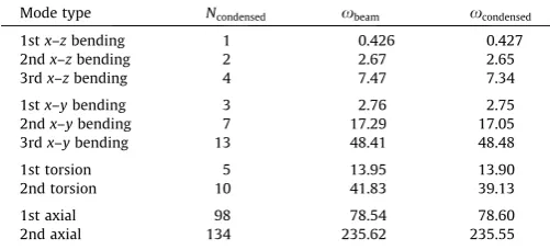
5.1.1. Comparison of natural frequencies and mode shapes
First, we will compare the LNMs obtained from the condensa-tion process with the analytical ones. This will serve to verify details of implementation, but also to highlight some characteris-tics, and advantages, of our approach.Table 1shows the natural frequencies on a set of modes selected to span the whole space of possible beam deformations. It includes the first three bending modes in each axis, and also the first two twisting and axial defor-mation modes, even if they have higher frequencies, so as to cap-ture in-plane deformations and 3-D rotations in the nonlinear beam dynamics. The table also includes the order number in which they appear in the reduced-set solution of the 3-D FEM model, Ncondensed. In practice, the process of selecting mode types can be
automated by ranking modes according to the total number
zero-crossings (nodal points) on the relevant component of the velocity modes, which should lead to better spanning of the space of possible deformations. This however has not been explored in this work.
As expected, bending and axial modes compare very well. The analytical model does not include warping restraint, and the differ-ences in the torsional modes are larger. Similar observations can be made of the mass-normalised mode shapes in intrinsic coordi-nates, which are shown inFigs. 3 and 4. As mentioned above, there is no need to compute the sectional compliance matrix,C, to nor-malise the component of the modes in stress resultants,U2, since
they are obtained from the same set of modes in displacements, U0, as the modes in velocities,U1. The effect of warping restraint
can be clearly seen on the torsional modes inFig. 4. It is important to emphasise that the constant-section beam solution is included here only as a reference: The nonlinear model obtained by the con-densation method is calculated in terms of mode shapes and fre-quencies directly obtained from the 3-D FEM. As a result, the present method, being based on an actual built-up geometrically-accurate model of the structure, naturally includes end effects due to kinematic restrictions along the longitudinal dimension.
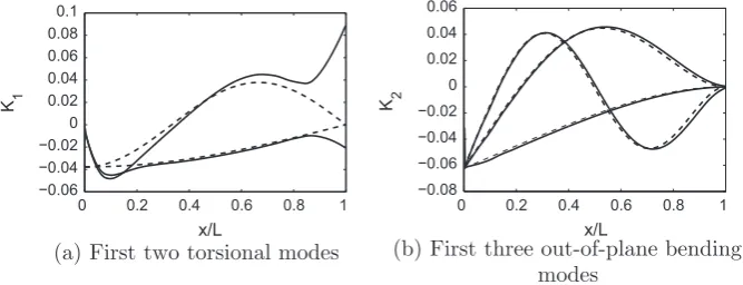
We still need to compute the productCU2jfor each mode shape.
This physically represents the force and moment strains (curva-tures) in the LNMs. The curvatures for the first out-of-plane bend-ing and torsional modes, obtained from Eq. (30), are shown in Fig. 5. Results are compared against the constant-section beam solutions. As before, bending modes compare well, while restrained warping on torsional modes is not included in the ana-lytical model and creates significant differences near the bound-aries, which increase with the frequency. At this stage, we can finally compute all the coefficients in the equations of motion in intrinsic modal coordinates, Eqs.(12).
5.1.2. Geometrically-nonlinear beam dynamics
Once the coefficients for the geometrically-nonlinear equations of motion have been identified, the dynamics of the condensed structure can be investigated. The simulations in this paper corre-spond to free vibrations for a parabolic initial velocity distribution, given asx1ðx;0Þ ¼x10ðx=LÞ2, wherex102R6will be the parameter
in the different test cases. An explicit 4th-order Runge–Kutta was used to solve the first-order intrinsic Eq.(12), with a time step Dt¼0:02 and no structural damping. Sectional velocities and stress resultants are then obtained using the modal expansions in Eq. (11). Finally, the material velocities are integrated at the point of interest using the equations of rigid body dynamics.
[image:8.595.311.562.96.210.2]Fig. 6shows the velocities and displacements at the free end of the box beam for small initial velocities, x10¼ð0; 0:002;0:002;0; 0;0Þ. In this case, the response is in Table 1
Selected natural angular frequencies from static condensation of the 3-D FEM and 1-D analytical solution.
Mode type Ncondensed xbeam xcondensed
1stx–zbending 1 0.426 0.427
2ndx–zbending 2 2.67 2.65
3rdx–zbending 4 7.47 7.34
1stx–ybending 3 2.76 2.75
2ndx–ybending 7 17.29 17.05
3rdx–ybending 13 48.41 48.48
1st torsion 5 13.95 13.90
2nd torsion 10 41.83 39.13
1st axial 98 78.54 78.60
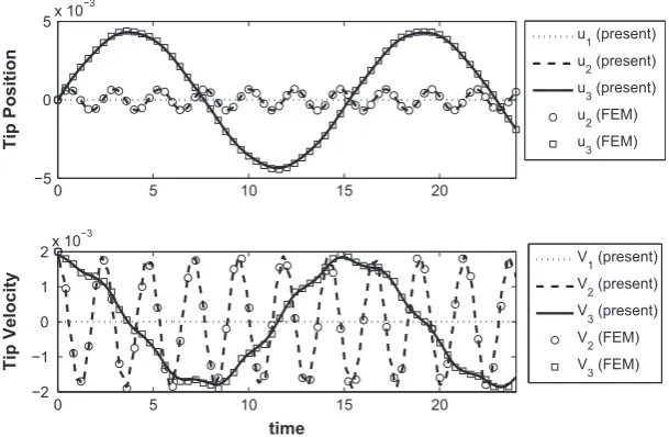
the linear regime and can be compared directly with that obtained using the condensation method developed in this paper. The intrinsic equations of the form(12), calculated via condensation
of the 3-D Nastran model, are based on the 10 modes shown in Table 1. Since these modes are directly obtained from the 3-D model, both methods are effectively solving the same equations,
0 0.5 1
−4 −2 0 2 4
V 3
0 0.5 1
−1 −0.5 0 0.5 1 1.5
Ω 2
0 0.5 1
−1 −0.5 0 0.5 1 1.5
F 3
x/L
0 0.5 1
−4 −2 0 2 4
M 2
[image:9.595.136.453.67.294.2]x/L
Fig. 3.Out-of-plane bending modes in intrinsic coordinates from the reduction from 3-D FEM (continuous lines) and a constant-section beam (dashed).
0 0.2 0.4 0.6 0.8 1
−3 −2 −1 0 1 2 3
V 1
0 0.2 0.4 0.6 0.8 1
−50 0 50
x/L
F 1
(a) Extension modes
0 0.2 0.4 0.6 0.8 1
−10 −5 0 5 10
Ω 1
0 0.2 0.4 0.6 0.8 1
−3 −2 −1 0 1 2 3
M 1
x/L
[image:9.595.130.457.337.513.2](b) Torsional modes
Fig. 4.First two axial and torsional modes in intrinsic coordinates from the reduction from 3-D FEM (continuous lines) and the constant-section beam model (dashed).
0 0.2 0.4 0.6 0.8 1 −0.06
−0.04 −0.02 0 0.02 0.04 0.06 0.08 0.1
K 1
x/L
(a) First two torsional modes
0 0.2 0.4 0.6 0.8 1 −0.08
−0.06 −0.04 −0.02 0 0.02 0.04 0.06
K 2
x/L
[image:9.595.127.461.559.687.2](b) First three out-of-plane bending
modes
except for very small differences due to the modal truncation in the intrinsic solution.
If the amplitude of the initial velocities is increased, geometrically-nonlinear effects become relevant.Fig. 7shows the displacements and velocities at the free end with x10¼ð0;2; 2;0; 0;0Þ. Maximum tip displacements in this case
are about 25% of the beam length. The first observation is that a lar-ger modal basis is needed to obtain converged results.Fig. 7 com-pares the results obtained using the 10 modes employed in the linear case (corresponding to those in Table 1), which were deemed sufficient for that problem, against a model built with the first 18 modes, plus the first two axial modes (N¼20), and a model with the first 50 modes. Note that the axial modes are included manually as the lowest axial mode is at number 98 (Table 1). This is necessary to introduce the nonlinear coupling between modes. The shift in the frequency of the in-plane motions is not captured by the small modal basis. The larger basis is not required in order to model the frequency content in the response as such, but rather because the mode shapes are needed to approx-imate the instantaneous deformed shapes in the nonlinear response. It can be shown analytically[32]that, if no axial modes were included, there would be no couplings in the deformations on the principal bending planes of the isotropic beam.
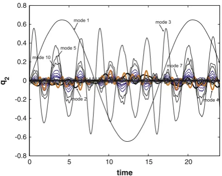
As it can be seen inFig. 7, results have converged forN¼20 and that system is further investigated inFig. 8, which shows the time history of the first 20 modal amplitudes (force component,q2) for
the same geometry and initial conditions. All visible modes in Table 1are identified. The response shows the nonlinearities pre-sent in the system, as a linear system would have exhibited a series of harmonic oscillators in the modal response. In particular, note that the torsional modes, which are not excited in the linear case, are rather significant and their amplitude is essentially modulated by the first bending mode in each plane. This finite-rotation effect occurs when there is simultaneous bending in both axes and disap-pears for planar deformations. A second effect of the nonlinear interaction is that the higher modes exhibit dynamics on a time-scale similar to that of the lower frequency mode, which links to the time-marching approach described in Section4.1.
Fig. 9compares the displacement at the centroid of the free end obtained from condensation with 50 LNMs, for large initial condi-tions x10¼ð0; 2;2;0;0; 0Þ, with those obtained from (1) the
constant-section intrinsic beam equations, (2) constant-section beam models in Abaqus, and (3) full 3D FEM in Abaqus. The con-stant section intrinsic modal solution also uses 50 modes on a 200-node beam with adaptive RK4 time-stepping and a relative error for convergence of 106. The Abaqus constant section
0 5 10 15 20
−5 0 5x 10
−3
Tip Position
0 5 10 15 20
−2 −1 0 1 2x 10
−3
time
Tip Velocity
u 1 (present) u
2 (present) u
3 (present) u
2 (FEM) u
3 (FEM)
V 1 (present) V
2 (present) V
3 (present) V
2 (FEM) V
[image:10.595.150.455.69.268.2]3 (FEM)
Fig. 6.Displacements and velocities at the free end for small initial velocitiesx10¼ð0;0:002;0:002;0;0;0Þ. Results from Nastran (FEM) and the present condensation
method.
0 5 10 15 20
−1 0 1
u 1
0 5 10 15 20
−1 0 1
u 2
0 5 10 15 20
−5 0 5
time u 3
N=10 N=20 N=50
(a) Displacements (in global coordinates)
0 5 10 15 20
−0.1 0 0.1
V 1
0
5 10 15 20
−2 0 2
V 2
0 5 10 15 20
−2 0 2
time V 3
N=10 N=20 N=50
[image:10.595.112.495.318.488.2](b) Velocities (in material coordinates)
finite-element beam solution is a converged geometrically-nonlinear solution (2000 B31 Abaqus elements and time step Dt¼0:01), whereas the Abaqus finite-element 3D solution uses 4500 S4 shell elements with a time step Dt¼0:02 and geometrically-nonlinear deformations. The full 3D FEM model has distributed mass and therefore cross-sectional constraints are added to prevent large sectional warping that would appear due to the initial condition. Very good agreement can be observed between both constant section beam models, which verify our implementation of the nonlinear intrinsic beam solver. Equally, the nonlinear solution on the full 3D FEM and that based on the static condensation also agree. The difference between the two sets of results can be seen in theu2response and the results show the
improvement obtained when deriving the beam equations directly from the 3D model, such improvements are mostly due in this particular case to the poor approximation to the torsional modes in the constant-section models.
Finally, Table 2shows the norm of the displacement vector error of tip displacement as a fraction of the maximum tip dis-placement between the full 3D model and the present method with 50 modes for different amplitudes of initial excitations of the formx10¼ð0;k; k;0; 0; 0Þ. The error shows that as the
max-imum tip displacementpz;maxincreases, the normalised error
even-tually increases due to the increasing effects of section warping not
captured in the condensation model. It should be also noted that the error arises mostly from a difference in frequency of the response and is otherwise minimal, as it can be seen inFig. 9.
5.2. Static condensation and dynamic response of an unsupported three-bar structure
This final test case is a U-shaped beam that was originally defined by Hesse and Palacios [7]. It consists of a free-flying U-shaped beam assembly with solid rectangular cross-sections subject to external loads. The shape of the structure is shown in Fig. 10(a) with isotropic sectional properties listed inTable 3. The applied forces and moments in Fig. 10(a) are Fz¼1000f;Fy¼100f;Fy2¼250fandMy¼100Lxf, where the load
profilefðtÞis shown inFig. 10(b). All applied forces are dead loads while the applied moments are follower loads that move with the local reference frame. As the position of the centre-of-mass of the free-flying structure under the influence of dead loads can be com-puted analytically, it offers a good test to assess the convergence requirements to preserve total momentum in the structure.
A finite-element model is constructed using a commercial FE analysis package (MSC NASTRAN v2012.1.0), shown inFig. 11(a). This model contains 4752 3D solid elements and 1–5 lumped mass condensation nodes per 5-m span (i.e., models with total model sizes of 7, 13, 19, 25 and 31 lumped mass nodes respectively). Lumped mass elements are connected to the massless structure using NASTRAN’s RBE3 interpolation elements, so that the spatial location of the lumped mass nodes are expressed as a linear com-bination of the closest nodes on the structure. Static condensation is then used to reduce the stiffness matrix to the degrees of free-dom associated with the lumped mass nodes. For comparison, beam models using equivalent 1-D sectional property definitions (Table 3) were constructed with the same number of nodes and the modal system is obtained in the same way as in the condensed model.
0 5 10 15 20
-0.8 -0.6 -0.4 -0.2 0 0.2 0.4 0.6 0.8
time
q 2
Fig. 8.First 20 modal amplitudes of the force component q2 for
x10¼ð0;2;2;0;0;0Þ. Modes 11–20 are shown in blue and all visible modes from Table 1have been identified. (For interpretation of the references to color in this figure legend, the reader is referred to the web version of this article.)
0 2 4 6 8 10 12 14 16 18 20
−0.04 −0.02 0
u 1
/ L
0 2 4 6 8 10 12 14 16 18 20
−0.05 0 0.05
u 2
/ L
0 2 4 6 8 10 12 14 16 18 20
−0.5 0 0.5
u 3
/ L
time
Const. Section ABAQUS Const. Section Intrinsic Present
[image:11.595.45.275.66.248.2]ABAQUS 3D
Fig. 9.Components of the displacements (in the global frame) atx¼L, forx10¼ð0;2;2;0;0;0Þ.
Table 2
RMS error between 3D FEM and present method of the vertical displacementpz(in
the global frame) atx¼L, forx10¼ð0;k;k;0;0;0Þ, normalised using maximum tip displacement.
k pz;max RMS=pz;max
0.002 0.004216 0.0306
0.2 0.4221 0.0303
1 2.1622 0.0242
2 4.5644 0.0131
3 7.2270 0.0105
4 10.0135 0.0205
[image:11.595.301.553.104.184.2] [image:11.595.134.455.581.738.2]Fig. 12shows the non-zero entries in the stiffness matrices of the beam model and the condensed model. It can be seen from the Figure that the stiffness matrix obtained from the condensation of the 3D FE model in the 31-node case is fully populated with sig-nificant non-zero entries far from the diagonal, whereas that from a beam model is banded with a very small bandwidth. The maxi-mum magnitude of entries in the fully populated stiffness matrix that are zero in the beam-based stiffness matrix is about 1% of the magnitude of entries within the banded matrix.Fig. 13shows the difference between the lowest 40 structural eigenvalues of the condensed model and the beam-element model for the 31-node problem.
The numerical results show that the root-mean-square differ-ence of centre of mass location vector with theory for models both built from prescribed beam elements and constructed using the
condensation method (simulated with full modal basis). The error scales, in this case, quadratically with element size (shown as the slope on the log–log plot inFig. 14). Thus the application of con-densation in creating the nonlinear modal system can achieve a similar level of conservation to the beam-element model. In this test case these are mainly discretisation errors that arise due to the linear velocity and piecewise-constant stress interpolations used in the model.
The effect of truncation and residualisation on the accuracy of the simulation is also studied with momentum conservation. Here the 31-node full-order model (total structural mode number NM¼180) is either truncated toNC lowest-frequency modes by
removing the remaining modes from the system, or residualised toNClowest-frequency modes by only removing the linear
dynam-ics of the remaining modes. Their effect on the accuracy of system momentum conservation is shown in Fig. 15(a). The maximum stable timesteps for the truncated and residualised system relative to the full-order system are the same and is shown inFig. 15(b). It can be seen that residualisation provides significantly better results compared to truncation for any given NC, while allowing
for the same increase in maximum permissible timestepDtmaxas
truncation, an increase that can be very significant.
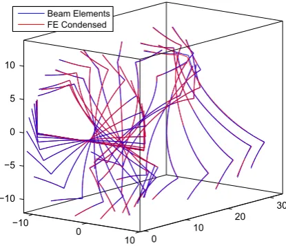
Snapshots of the shapes of the deformed beam during the first 15 s of time-marching simulation using the condensed and beam element approach, both with 31 nodes, are shown in Fig. 16. Although both models are obtained by completely different pro-cesses, their responses are still very similar. As it can be seen in Fig. 13, the difference in the lowest structural eigenvalues between the condensed model and the beam-element model for the 31-node problem is small. For longer time integrations the small
[image:12.595.133.480.69.199.2]Table 3
Table of properties and equivalent sectional properties of the isotropic free-flying structure[7].
Cross section 0:10:05 m rectangular
E 70 GPa
m 0.3
q 2700 kg/m3
EA 3.5e8 N
GJ 140224.3 N m2
EI2 291666.7 N m2
EI3 72916.7 N m2
qA 13.5 kg/m
qmI1 0.0140625 kg m
qmI2 0.01125 kg m
qmI3 0.0028125 kg m
(a) The 4752-element FE model
con-structed according to the material
def-initions in Table
3
.
−5 0 5 10 −15
−10 −5
0 5
10 15 −5
0 5
(b) The 31 analysis nodes in Figure
11(a)
with the interconnecting load path
also shown.
Fig. 11.The 3D solid-element and corresponding 1D model of the U-shaped beam.
F z
M y
F y
F y2
M y
F y P
L x = 20m
F z z
x y
(a) Initial configuration of the structure shown
with 31 nodes. Applied forces and moments are
also indicated.
0 5 10 15 20 25
0 0.5 1 1.5 2
Time / s
f (t) / N
(b) Time-varying load profile
f
(
t
) applied as forces and
mo-ments on the structure.
[image:12.595.46.292.265.379.2]differences between models (as seen in the eigenvalues inFig. 13) accumulate to give slowly diverging trajectories.Fig. 17plots the response of the 31-node, statically condensed model together with data from a converged solution using beam elements from SAMCEF Mecano (from[7]), the comparison demonstrates that the response is captured to a good degree of accuracy by the condensation tech-nique. The difference between them arises due to the differences present in the linear normal modes between the methods, in par-ticular the capturing of end effects by the reduction method, which is then amplified by the large, geometrically nonlinear motions
that the structure underwent. Snapshots of the shapes of the deformed beam during the first 15 s of time-marching simulation using the condensed and beam element approach, both with 31 nodes, are shown inFig. 16. Although both models are obtained by completely different processes, their responses are still very similar. As it can be seen inFig. 13, the difference in the lowest structural eigenvalues between the condensed model and the beam-element model for the 31-node problem is small. For longer time integrations the small differences between models (as seen in the eigenvalues inFig. 13) accumulate to give slowly diverging tra-jectories. Fig. 17 plots the response of the 31-node, statically
Beam Model
50 100 150
50
100
150
Condensed FE
50 100 150
50
100
[image:13.595.142.444.69.223.2]150
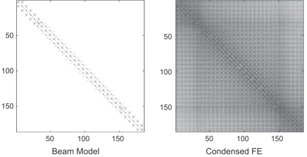
Fig. 12.A comparison of sparsity of stiffness matrixKacomputed from beam elements and a Guyan reduction on 3-D FE model. Both models contain 31 nodes. Dark dots
indicate a non-zero entry where shading implies higher magnitude.
0 10 20 30 40
0 1 2 3
Mode Number j
Relative Difference in
ω j
[image:13.595.331.522.275.391.2](in %)
Fig. 13.Relative difference in the lowest structural eigenvalues between the
condensed system and the beam-element solution for the 31-node model.
100 101 102
10−3
10−2
10−1
100
Element Count
δ
r CM
/ m
Intrinsic Beam Elements Guyan Reduction Quadratic Best Fit
Fig. 14.Error in c.m. location between computed and analytical results over a
simulation period of 20 s. Both the condensed model and the beam-element model are shown. The line for cubic error reduction with element number is also indicated.
0.2 0.4 0.6 0.8 1
0 0.5 1 1.5 2
N C / NM
δ
r CM
/ M
Residualisation
Truncation
(a) Effect of truncation and residualisation
on the accuracy of c.m. location over a
simulation period of 20
s
.
0.2 0.4 0.6 0.8 1
0 5 10 15 20 25 30
NC / NM
Δ
t max
/
Δ
t max,full
(b) The
maximum
stable
timestep
[image:13.595.58.261.277.399.2]Δ
t
maxfor the truncated / residualised
system, relative to the full-order system.
[image:13.595.43.276.451.596.2]condensed model together with data from a converged solution using beam elements from SAMCEF Mecano (from[7]), the com-parison demonstrates that the response is captured to a good degree of accuracy by the condensation technique. The small differences between them arises from the slightly different estima-tion of the linear normal modes between both methods, which is then amplified by the long time integrals.
To summarise, the numerical cases in this chapter demon-strated the process of static condensation via Guyan reduction combined with the intrinsic formulation in creating a nonlinear modal structural system from a 3D FE model.
6. Conclusions
This paper has introduced a procedure to obtain modal-based geometrically-nonlinear descriptions from detailed 3-D finite-element models of structures with lumped inertia and slender sub-components. The condition for this is that a static con-densation in the structural model is carried out into grid nodes along the main load paths in the original structure. This is in fact just exploiting the usual approach to obtain stress resultants in air-craft load analysis. Subsequently, the spatial distribution of those
analysis nodes is used to construct 1-D representations of the mode shapes.
The formulation works in a global basis and it directly uses the linear normal modes of the reduced structure. As a result, there is no loss of accuracy in linear analysis beyond that of the condensa-tion. It is intrinsic, which means that it transforms the mode shapes from nodal displacements and rotations into their spatial derivatives (strains, or internal forces) and time derivatives (veloc-ities). Those are local magnitudes which decouple the computation of local stiffness and inertia with spanwise (integral) geometrically-nonlinear effects. A direct consequence of this is that only linear calculations are required on the large 3-D model, while the geometrically-nonlinear effects are included by the spatial dis-tribution of the analysis nodes. This is a substantial advantage with respect to methods based on projections of the displacement field, which require full nonlinear solutions. Moreover, the intrinsic equations only include quadratic nonlinear terms, which allows computationally-efficient numerical procedures on complex structures.
Numerical results have been presented for a cantilever box beam and a three-bar structure. It is first shown that the nonlinear equations of motion can be built directly from the shell model and it has also shown that obtaining the nonlinear coefficients from the direct computation of 1-D strains and curvatures for each mode removes the need for estimation of the sectional compliance matrix. Results for the cantilever box beam were presented against nonlinear beam models and the proposed description has the abil-ity to capture torsional deformations arising from the nonlinear couplings under large amplitude vibrations. The airframe model further demonstrated that this technique is applicable to a more complex structure and that geometrically nonlinear time-domain analysis can still be performed on such a model. It was also shown that the computational speed of the current method can be effec-tively controlled via approximation of high-frequency dynamics as algebraic equations, while still retaining excellent accuracy and geometrically nonlinear couplings.
To conclude, the proposed method allows the generation of geometrically-nonlinear reduced-order models of complex (but slender) structures as a non-intrusive post-processing step of a lin-ear vibration analysis. It produces first-order equations of motion with quadratic nonlinearities that can be time-marched at a rela-tively modest computational cost.
Acknowledgements
The second author would like to thank Professor Moti Karpel, from the Technion, for many enlightening discussions to establish the links between the present model-reduction method and air-craft load analysis procedures. The work is partially supported by the UK Engineering and Physical Sciences Research Council Grant EP/I014683/1 ‘‘Nonlinear Flexibility Effects on Flight Dynamics and Control of Next-Generation Aircraft’’.
References
[1] Noll TE, Ishmael SD, Henwood B, Perez-Davis ME, Tiffany GC, Gaier M, et al. Technical findings, lessons learned, and recommendations resulting from the Helios prototype vehicle mishap. In: NATO/RTO AVT-145 workshop on design concepts, processes and criteria for UAV structural integrity. Florence, Italy; 2007.
[2] Bazilevs Y, Hsu M-C, Kiendl J, Wuchner R, Bletzinger K-U. 3D simulation of wind turbine rotors at full scale. Part II: fluid-structure interaction modeling with composite blades. Int J Numer Meth Fluids 2011;65(1–3):236–53.http:// dx.doi.org/10.1002/fld.2454.
[3] Bazilevs Y, Hsu M-C, Kiendl J, Benson D. A computational procedure for prebending of wind turbine blades. Int J Numer Meth Eng 2012;89(3):323–36. http://dx.doi.org/10.1002/nme.3244.
−10
0
10 0
10 20
30 −10
−5 0 5 10
[image:14.595.64.272.67.245.2]Beam Elements FE Condensed
Fig. 16.Dynamic response of the structure in the first 15 s when subjected to the
prescribed forces and moments shown inFig. 10(a). This figure shows the difference between that of a system computed from 1-D beam property definitions and that of a model from a static condensation of 3-D FE buildup.
0 5 10 15 20
−20 0 20 40 60 80
t / s
r / m
rx,g
ry,g
rz,g
rx,ref
ry,ref
rz,ref
Fig. 17.Comparison of the response inFig. 16for the spatial location of point P in
Fig. 10(a) for the reduced model from static condensation (rg) and converged
[image:14.595.52.287.316.466.2]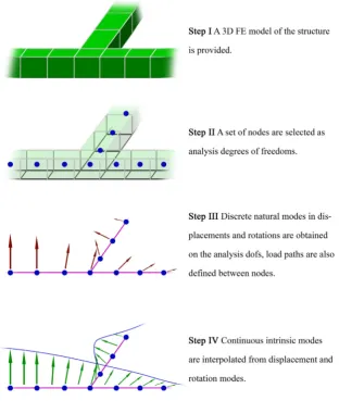
![Fig. 10. Three-bar structure and applied loads (after Hesse and Palacios [7]).](https://thumb-us.123doks.com/thumbv2/123dok_us/9514208.456808/12.595.133.480.69.199/fig-bar-structure-applied-loads-hesse-palacios.webp)