I. T. Pearson and J. T. MOTTRAM, ‘Finite element modelling methodology for the non-linear stiffness of adhesively bonded single lap-joints. Part 1. Evaluation of key parameters,’ Computer and Structures, pp. 13.
ISSN 0045-7949 doi:10.1016/j.compstruc.2011.10.005 (online)
A finite element modelling methodology for the non-linear stiffness evaluation
of adhesively bonded single lap-joints. Part 1. Evaluation of key parameters
Ian T. Pearson* and J. Toby Mottram2 WMG1 and School of Engineering2
Warwick University Coventry CV4 7AL
ABSTRACT
Reported in this paper is the development and verification of a finite element model with the fewest solid elements that can predict the non-linear stiffness characteristics of adhesively bonded single lap-joints in vehicle bodies. This work was driven by the need to significantly reduce computing hardware resources and run times for whole body analyses, and to achieve this goal the lap-joint needs to be modelled by a ‘small’ number of shell elements. It is well-known that the deformation of bonded lap-joints is dependent on seven key parameters, and that it is impractical to have a comprehensive characterisation of these by physical testing alone. To gain further understanding of the influence of these parameters on joint stiffness, over a wider range of variables than could be practically achieved in the laboratory, the ANSYS finite element code is used to simulate the highly non-linear (geometric and material) response of bonded joints. The authors use the laboratory results for joint stiffness from nineteen batches of laboratory specimens to aid the development, and verification, of numerical derived stiffness curves from a solid element model. Initially, a very refined mesh is used. This model is developed to have a ‘coarse’ solid element mesh that minimises run times without the calculated joint stiffness deviating by more than 10% from the batch mean
of 10 measurements from laboratory testing. Numerical results from many simulations using the ‘coarse’ solid mesh model are used to show that, for the shell modelling methodology (reported in Part 2 on this work) to be successful, a representative model must account for the four key parameters of: adherend stress-strain relationship, adherend thickness, bond line thickness, and the over lap length. The ANSYS results also confirm that stiffness is directly proportional to joint width.
Key Words: Finite element, joint, adhesive, stiffness, non-linear, vehicle body design a Corresponding author: E-mail [email protected]
INTRODUCTION
When the decision is made to introduce a new vehicle model, a principal requirement to be considered is how to accurately simulate the body’s overall torsional and bending stiffnesses in computational analyses. As we know the body is constructed by joining together numerous thin walled metallic panels, and so the choice of joining technique (e.g. continuous welding, resistance spot-welds, rivets and nuts and bolts, etc.) and joint detailing will greatly influence local and global stiffnesses. The international requirement for an unremitting reduction in automobile body weight is sought to pacify the calls for increased fuel efficiency. The need for body design optimisation (requiring minimum weight) has therefore been driven by the Corporate Average Fuel Economy (CAFE) Regulations [1] of North America and by a proposed European Carbon Tax [2]. Traditionally, weight reduction in a vehicle’s structure has been achieved by: having a reduction in material thickness, using lightweight materials, introducing innovative hybrid structures, or a combination of these. Another option that is attractive is to replace the traditional joining techniques (listed above) with continuous adhesive bonding; as bonded joints will either increase body stiffness or provide the same stiffness when utilising thinner, lighter panels.
spot-welding aluminium alloys is a relatively expensive option and is clearly impractical with polymeric composites.
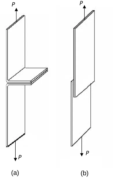
The coach joint geometry shown in Figure 1(a) is optimised for ease of assembly by spot-welding, and so it is often found in current automobile body detailing. The inability of an adhesive layer to tolerate the ‘peel’ stress field generated when joints of this geometry are loaded makes it undesirable. Instead we find that the single lap-joint geometry, shown in Figure 1(b), is more appropriate to utilise the adhesive’s ability to resist shearing, and to reduce the abhorrent peel stresses that exist in the coach joint. Single lap geometries still suffer from what Hart-Smith [4] calls ‘parasitic’ peel loading, because the line of action of the force in the two adherends has a load path eccentricity. The reality is that peel forces can be reduced by detailing, but never eliminated, and their associated ‘through thickness’ stresses are often what causes premature joint failure.
The final objective of the research reported in Parts 1 and 2 [6] is to develop a finite element (FE) modelling methodology that will enable a very small number of shell elements (using ANSYS) to simulate the non-linear stiffness response of bonded lap-joints and be suitable for inclusion in existing automotive shell element models. Other FE modelling researchers [7-9] have formulated special adhesive joint elements, but none of these are to be found in commercially FE codes [10]. Modelling a relatively thin adhesive layer (< 1 mm thick) with solid (brick) elements produces models with too many degrees of freedom (d.o.f.), especially when appropriately sized elements are used to model the remainder of the structure [11]. To achieve a model with acceptable number of d.o.f. there is an intermediate objective to complete, whereby we establish that FE analysis can predict sufficiently reliable joint stiffness characteristics, to ultimate failure, for the practical range of the seven key parameters known to have an influence. To assess the FE results, from ANSYS analyses, a series of laboratory tests have been performed and measured stiffness characteristics from them are reported herein.
For the lap-joint with the benchmark properties (geometry and material properties are given in first row of Table 1) a solid finite element mesh with 11 elements through the thickness of the bonded overlap length is required to show that numerical results for the non-linear joint stiffness are close to those measured. The word benchmark is used to identify the joint details from which variations to the key parameters can be specified. Because there is no known optimisation approach to minimise the number of d.o.f., a trial and error procedure is used to reduce the number of solid elements (now with eight elements through the thickness) so that a solid model, taking 1/5th of the run time, still gives acceptable predictions. This second solid mesh is referred to in this paper as the ‘coarse’ solid model. By using this resource-efficient model, after it had been verified, the authors conduct an extensive computational parametric study to be able to determine the influence of each the key design parameters over a wider range of values than could be practically, and economically, achieved in the laboratory.
it is now feasible for the stress analyst to include bonded single lap-joints (Figure 1b) in a whole vehicle FE model.
LABORATORY TESTING FOR JOINT STIFFNESS
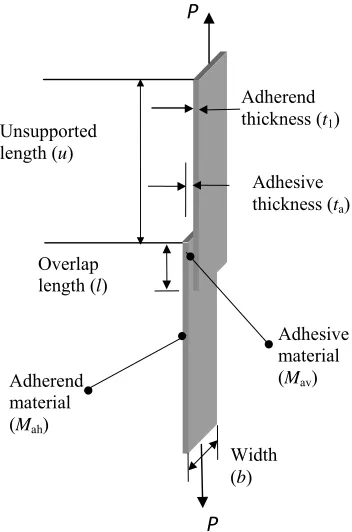
Seven key parameters known to influence joint stiffness where chosen for consideration in the series of laboratory tests. Two of these parameters are the stress-strain relationships for the adherend and adhesive materials. Specific dimensions for the other five key parameters are given in Table 1 (and defined in Figure 2). Their choice followed a review of the work by Wooley and Carver [12] who had investigated the stress distribution within the adhesive layer on varying the adhesive modulus, the bond line thickness and the overlap length, and by Li et al [13] who showed that changes in the adhesive’s thickness changed the joint stiffness. From a study on the Stress Intensity Factor (SIF) by Goglio and Rossetto [14] it has been shown that, as the overlap length increases, so the SIF decreased and this causes an increase in joint stiffness. These researchers also found that the influence of bond line thickness on stiffness to be very dependent on the choice of local joint geometry.
The original plan of the research had been to complete two laboratory series of comparable joint tests with adherends either of a grade of steel (BS) and of an aluminium alloy (LR). This was not practical because of the metal thicknesses available. The well-known design of experiments technique has not been employed, as it is more important, to the aims of the work, to be able to identify the real physical effect of varying individual key parameters rather than to save time (and minimise costs) when conducting the series of laboratory tests. Additionally, for the design of experiments technique to work the joint stiffness has to vary linearly between the ‘high’ and ‘low’ values chosen for the key parameters. The results presented later will show that there are non-linear relationships between the chosen ‘high’ and ‘low’ values for the seven key parameters.
restricted testing to, first, investigate the influence of thickness change for aluminium (with the two thicknesses of 1.2 and 1.6 mm) and second to assess the effect of having 0.8 mm thick adherends of steel, while changing the other six key parameters given in Table 1.
For the six parameters that are changed in the joint tests, Table 1 gives the benchmark joint value in row one and either another value or two values in row two. Values for adherend thickness (t1), overlap length (l) and adhesive thickness (ta) were chosen as being typical of those found in automobile manufacture. The unsupported length (u) is an unknown parameter in terms of manufacture; it is a variable specific to the lap-joint test. No application measurements are known for this dimension and so 50 mm was chosen as being convenient and practical for the purpose of physical testing. Similarly, the width of the joint (b) was conveniently chosen at 25 mm. The benchmark adhesive was taken to be product MA310 (a low modulus ‘rubbery’ methacrylate from ITW Plexus) and an alternative in the parametric study was a commercially available adhesive (Araldite Precision, a two-part cold cure, ‘glassy’ epoxide supplied by CIBA-Geigy Ltd). The two adhesives for this work were chosen because they represent a range of adhesive material properties that is likely to encompass those adhesives used by vehicle manufacturers.
When testing joints with the aluminium adherends the benchmark t1 is 1.6 mm. For both metal adherends the other benchmark and variant parameter values in this series of tests are those listed in row one of Table 1.
A batch of nominally identical specimens was manufactured by the first author with the benchmark values (for the benchmark aluminium joint). Nine further batches, for the so-called ‘parametric’ aluminium joints, were prepared, in which values for five of the six key parameters remained as in the benchmark, and the other parameter was taken from the variant list in row two of Table 1. This process for generating joint batches was repeated for the benchmark steel joint and its associated ‘parametric’ steel joints. As only one adherend thickness was used there are eight ‘parametric’ steel joint batches involved in the laboratory testing for the non-linear joint stiffness.
the secondary deformations from the eccentric loading [4] there were bonded end tabs of the same metal thickness at both ends of the joint. This specimen feature is shown in Figure 3. When bonding the adherends, and end tabs, surplus adhesive was removed from the sides and ends, leaving the specimen without noticeable spew fillets. It is known that the actual geometry of the spew fillet at the overlap ends can significantly alter the failure load due to adhesive rupture [15], but for stiffness characterisation this detailing is not important. The adhesive thickness was regulated at 0.3 mm (for the benchmark joints) by adding glass beads (known as ballotini) of this diameter to the adhesive on application. For the thicker bond layer of 1.6 mm (Table 1 row two) thickness control was achieved with short lengths of copper wire of that diameter. Care was taken to orientate and position these spacer wires sufficiently far away from the sides of the joint and so avoid a possible premature failure due to the interaction of edge stress fields and wire. The presence of the wire is not believed to have adversely affected the reported measurements for the non-linear stiffness response.
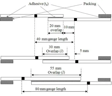
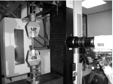
Specimen ends were gripped by conventional wedge grips in a 10 kN Instron testing machine. A displacement rate of 0.2 mm/s was applied until a specimen ultimately failed, with the mode of failure being adhesive rupture. A video (non-contacting) extensometer from Messphysik Laborgerate GES.m.b.H (type ME-45 Video extensometer) was used to record the axial displacement over a gauge length of the joint. The experimental set-up is seen in Figure 4. The video extensometer requires markers, or targets, to be attached to the specimen (Figure 3), and these must be equi-spaced either side of the overlap length. For convenience, this gauge length was set to 40 mm with the benchmark joints (where l = 20 mm), and this distance was acceptable with the variant overlap length of 30 mm. A target separation of 40 mm was however impractical for the other variant overlap length of 55 mm (Figure 3), where an increased video extensometer gauge length of 80 mm was found to be expedient.
of the finite element results. Based on the benchmark aluminium joint it is estimated that a displacement error of about 5% might occur when the joints are subjected to tension (P) sufficient to generated gross adherend plasticity, and this occurs before the lap-joint ultimately fails by adhesive rupture.
The two marker distances used with the three overlap lengths are shown in Figure 3.
LABORATORY
TEST
RESULTS
Next we shall discuss the laboratory test results in terms of changing one parameter (of the six key parameters given in Table 1) at a time. The objective of the parametric study is to identify their relative importance to the non-linear joint stiffness response, but it will also provide data for the verification of FE models.
The stiffness/load curves plotted in Figures 5 to 10 are derived from the best mean fits (i.e. polynomial representations fitted in a ‘least squares’ sense) to the ten test results (force/displacement) per batch. To report the results it is convenient to normalise the stiffness (ordinate axis) and tension force (abscissa axis) by dividing their measurements by the actual width of the joint. The justification for this will be given next. Note that P, in Figure 1, can be taken to be either the total tension force or the tension force/per unit width; when determining the applied tension stress the associated area is to be calculated accordingly.
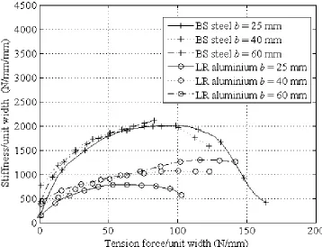
It has already been mentioned that the specimen width, at maximum 60 mm, is much smaller than the 1000 mm or longer that can be found in vehicle body constructions and the influence of this parameter is of primary importance for the production of a joint representation (Part 2 of this work) since if this is not linear, the width of the joint to be analysed will have to be known and incorporated in the replacement methodology. Results in Figure 5 from testing the three chosen joint widths (b) of 25, 40 and 60 mm (with the other five parameters being defined by their benchmark values) are plotted in Figure 5.
in Figure 5 suggests that a width of 20 mm, or higher, would be adequate to represent the continuous long widths found in vehicle body constructions. This finding is, moreover, an aid to the FE analysis as stiffness has been found to be directly proportional to width. This allows a ‘joint stiffness per unit width’ to be used for any specified joint width. Having established from the Figure 5 results that stiffness is directly proportional to width, the curves in Figures 6 to 10 are normalised by the width parameter (b). Joint stiffness per unit width (with units of N/mm/mm) is therefore plotted against increasing tension per unit width (with units of N/mm).
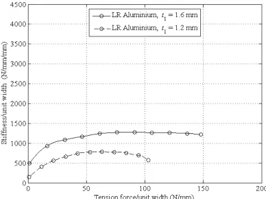
Only a single comparison for a change in adherend thickness (t1) was possible and its change is shown by the two curves in Figure 6. It can be seen that until the force per unit width exceeds 2 N/mm the stiffness itself cannot be determined from the video extensometer measurements. From the non-linear curves in this figure it can be observed that stiffness is dependent on adherend thickness and the force per unit width. A maximum stiffness of 1300 N/mm/mm is achieved with t1 equal to 1.6 mm and a lower value of 800 N/mm/mm when t1 is 1.2mm. This indicates that an increase in aluminium thickness of 33% has produced an increase in maximum joint stiffness of 60%. Had stiffness been based on axial deformation only, this change would be proportional to the change in cross-section area, that is, it would be linearly dependent on thickness. It is to be understood that a contribution to the measured joint stiffness is generated from the rotational deformation over the length of the overlap length caused by the moment from the eccentric load path, and this reduces in magnitude as the tension increases. Increased loading produces the flat proportion in the stiffness curve that shows us when the non-linear stiffness is controlled by the existence of gross metal plasticity at the ends of the overlaps.
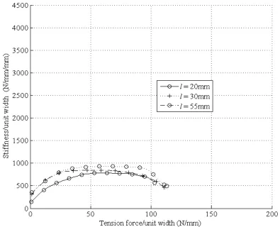
Presented in Figure 7 are the results for the aluminium joints (ta = 1.2 mm) with overlap lengths (l) of 20, 30 and 55 mm (with the other five benchmark key parameters unchanged). Based on the mean of the laboratory test results we find that stiffness is fairly insensitive to a change in l. It is known that on loading the stress distribution in the adhesive layer, and along the overlap length, will soon become highly non-linear, with plasticity regions forming and growing from the ends. However, even with the shortest overlap of 20 mm, the onset of adhesive plasticity in the central region only occurs shortly before ruptures. It can be seen from the curves in Figure 7 that the force per unit width when the joints rupture is similar. Although the value of overlap length does not significantly change joint stiffness it is recognised that its design value remains a very important parameter, especially when we need to specify a minimum dimension for l to design against loss of structural integrity due to durability, creep and fatigue [17, 18]. In other words the longer l is the higher will be the level of damage tolerance available to long-term affects that will weaken the joint.
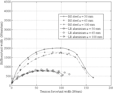
From the six plots in Figure 8 it can be seen that a change in unsupported length (u) from 50 to 100 mm has little influence on stiffness characteristics. As expected there is a batch mean trend towards increased stiffness with a decrease in the unsupported length from 100 to 50 mm; the increase is bigger for the joints of BS steel. As the unsupported length increases, joint deformation is governed by the relative stiffness of the unsupported adherend sections compared to the bonded overlap length. This justifies why the stiffness in Figure 8 is found to decrease with increased u. The rapid loss in stiffness with steel, for loading > 100 N/mm, is due to increased flexibility in longer adherends. The longer the adherends are the less they able to provide flexural stiffness to oppose the action of the bending moment generated by the load path eccentricity.
The stiffness curves in Figure 10 for change of bond line thickness (ta) confirm that a thinner layer gives a stiffer joint. An increase in ta allows a greater depth of adhesive to be in shear and causes an increase in load path eccentricity, thereby causing a higher bending moment at the same value of P. Thicker bond lines therefore induce higher stresses and larger axial deformations, and this is exhibited in Figure 10 by a lower mean joint stiffness.
USEFUL FINDINGS FROM THE LABORATORY TESTING
Changes to three of the key parameters investigated in the laboratory study (unsupported length (u), adhesive elasticity (Mav) and width of joint (b)) are found to have an insignificant influence on joint stiffness. It is important that stiffness is found to be unaffected by changes in width as this suggests the behaviour of actual vehicle body joints (perhaps a metre wide) can be predicted from tests on coupon specimens (typically, having a width of 25 mm).
Test results from the parametric study in Figure 5 to 10 indicate that it would be a challenge from the laboratory test programme to rank the key parameters in order of influence on joint stiffness. For the single lap-joint configuration it is found that stiffness increases as:
adherend thickness increases
adherend’s modulus of elasticity increases bond line thickness decreases
overlap length decreases.
DEVELOPMENT OF SOLID FINITE ELEMENT MODELS
For the purpose of obtaining greater understanding on the influence of varying the seven key parameters on the stiffness of adhesively bonded single lap-joints a FE parametric study was undertaken. The ANSYS finite element code was first used to model and analyse the highly non-linear (material and geometry) deformation response of the tensile loaded joints in the laboratory programme.
0.3 mm and the adhesive’s Poisson’s ratio of 0.4. For the benchmark joint the adherend material is BS steel, having the true stress/true strain relationship shown in Figure 11. The other three stress-strain curves in this figure are used to provide a parametric variation for key parameter Mah. The metals are assumed in the FE modelling to be perfectly plastic after attaining their maximum true stress, and this material constitutive modelling is shown in Figure 11 by dashed lines. The stress-strain curve for LR Aluminium was measured for this work [19], the data for the EN AW 6082 material curve was taken from the work by Wang et al. [20], and that for DP600 came from The Automotive Steel Design Manual [21].
The true stress/true strain curves for the four adhesive materials used in the FE parametric study are plotted in Figure 12. For non-linear analyses their constitutive stress-strain relationships are defined using a multi-linear material model for curve fitting. Data for adhesive MA310 are taken from the work by Dean et al. [22]. The other stress/strain curves in Figure 12 were used for parametric variation to key parameter Mav. The relationship for ESP105 was taken from work by Crocombe and Bigwood [23], whilst the curve for F 241 came from Dean and Duncan [24] and that for the Araldite Precision adhesive was obtained experimentally by the first author [19], following the method detailed in the paper by Dean and Duncan [24]. Again, these materials are assumed to exhibit perfect plasticity after yielding. For linear analyses, the results of which are compared against the non-linear analysis results, the constant modulus of elasticity in the first row of Table 2 is used.
The next step in the FE work is to find out how many of the solid elements in the refined mesh can be removed, without too much loss in numerical reliability. The solid element mesh shown in Figure 13 was made ‘coarser’ in stages, with the aim of maintaining acceptable confidence in the computational results for a significantly shorter solution time. By an iterative process [19] it was found that the coarser mesh shown in Figure 14, having two solid elements for the adhesive thickness and three for the adherend thickness would compute the axial displacement within 2% of that given by the refined mesh (Figure 13) simulation, but with a solution time of 1/5th. The main reason for this reduction is that the coarser mesh model has less than 6% of the total number of d.o.f. Having optimised the mesh specification the authors used the coarser solid model to investigate the influence of the key parameters over a wider range, see Table 3 for values, than could practically be covered by the laboratory testing. This parametric study is used to establish the magnitude of the influence of each key parameter on joint stiffness. It is noteworthy that with about 0.4k d.o.f. per mm width of joint the coarse mesh of Figure 13, even after minimising the number of solid elements, also has far too many d.o.f. for application in whole vehicle FE models.
VALIDATION OF THE COARSE SOLID MODEL
The true stress-true strain curves for adherends materials used in laboratory testing are shown in Figure 11, where the aluminium alloy is labelled LR Aluminium and the steel is identified as BS Steel. The non-linear tension-axial displacement response of the benchmark steel joint and the benchmark aluminium joint are presented in Figure 15 using a solid line for FE results and a dashed line for the mean batch test results. As can be seen there is, as could be anticipated, a fairly close agreement over the full load range. Figure 16 shows the stiffness per unit width against tension P for steel.
Note that the main reason for developing the coarse mesh was to be able to carry out a comprehensive parametric study on non-linear stiffness of bonded single lap-joints in a sensible period of time. It is observed in Figure 16 that the FE curve for the benchmark steel joint lies within the bounds formed by this level of uncertainty and so provides sufficient incentive for the continuation of the development of new FE models for bonded lap-joints [19]. Curves from the benchmark aluminium joint produced similar results [19].
In Figure 16 there is a more than acceptable correlation for P > 900 N, whereas for lower tension the difference can be attributed to the experimental challenge of determining where the displacement origin begins when using the ME-45 Video Extensometer to determine axial extension. It is likely that, had the actual displacement shift been known, the correlation would be even better than can be demonstrated herein. As a consequence of this instrument weakness the test measurements are more suspect when P is low, say < 900 N (uniform tensile stress in adherends of < 45 N/mm2).
The other steel joints defined in Table 1 were simulated using the same coarse solid model in Figure 14 and produced acceptable correlations that are reported in reference 19.
The equivalent parametric study with adherends (ta = 1.2 mm) of LR aluminium alloy also gave close agreement for the non-linear stiffness characteristics with increasing P, but for brevity they are not included here. This comparison [19] did however show that the computational predicted material plasticity occurs at P = 2000 N (or 40 N per mm width), this being 500 N below that measured. This divergence leads to a premature and higher loss of joint stiffness as given by the FE results. The explanation for this is that the yield strength (previously determined by laboratory testing) for the LR Aluminium in Figure 11 is lower than that for the same alloy used in the series of lap-joint tests [19]. In all cases the mean batch joint stiffness curves are shown by Pearson [19] to correlate well with the FE curves for changes to the key parameters of adherend thickness (t1), joint overlap (l), unsupported length (u), adhesive material (Mav), bond line thickness (ta) and joint width (b).
COARSE SOLID MODEL RESULTS AND DISCUSSION
properties (for adhesive and adherends), and every FE analysis included geometric non-linearity. Figures 17 to 20 and 22, 23 and 25 give plots of stiffness per unit width against tension force per unit width from both linear and full non-linear analyses, with the constant linear elastic results given by the dashed lines and the non-linear varying stiffnesses given by solid curves. Since changes in parameters are not limited to the laboratory test results, the modulus of elasticity of the adhesive is taken to be in the range 0.1 to 10 GPa. The justification for using a range beyond that given by the adhesives used by manufacturers was that the research had indicated that joint stiffness was not sensitive to either the value of the adhesive’s modulus of elasticity or to the localised bond line yielding at the overlap ends. The discussion on the parametric study results will be given in the context of the findings that are relevant to the development, and evaluation, of a simplified shell model that enables the non-linear joint stiffness to be incorporated into whole vehicle FE models. This new modelling methodology is the subject of Part 2 of this work [6].
The first parameter to investigate by FE analysis is joint width (b). In vehicle bodies a lap-joint can be a metre or more in width, significantly greater than the width of the standard test coupon, at 25 mm. Because of free edge effects it can be expected that as the width tends to zero there is to be a change in the stiffness response. If stiffness per unit width can be shown to be independent of b then a single representation is valid for all joint widths. In the FE study the four widths chosen are 25, 40, 60 and 80 mm. As their full non-linear curves, plotted in Figure 17, are concurrent it is confirmed that stiffness is directly proportional to joint width. It is however to be understood that this beneficial finding is valid until the load causes adherend plasticity. The onset of this material non-linearity is dependent on ‘applied load per unit width’, and for b = 25mm it occurs (point A in Figure 17) when P > 3500 N (or 140 N/mm). By choosing to stop the computational analyses at a constant tensile force of P = 3500 N, and plotting results in ‘force per unit width’ the other three curves terminate before there is yield failure. This explains why adherend plasticity at widths > 25 mm is not presented in Figure 17.
eventually causes section plastic deformation, and this is signified by a loss in joint stiffness. It can also be seen in Figure 18 that due to this thickness effect, and the non-linear response, the stiffness peaks in the load range 20 to 160 N/mm. It then starts to fall at a higher tension, which increases with increase in t1. The results in the figure show that the difference between linear and non-linear analysis increases faster when the adherends are their thinnest. A linear elastic analysis for t1 < 1.6 mm is always incorrect, and the error increases with load P. For t1 = 0.8 mm and P = 3500 N (140 N/mm) the peak difference between the two FE analyses is 52%. At the upper limit of adherend thickness (t1 = 2.0 mm) the maximum difference between the two computational analyses is only 11%, when P = 3750 N (150 N/mm). It is concluded from this particular parametric study that stiffness depends on t1. This key parameter must be included in the required shell element modelling methodology. This is developed in Part 2, where a mesh possessing the fewest shell elements, to offer the vehicle FE analyst the smallest number of d.o.f. per mm width, is developed and validated.
In Figure 19 there are two groups of plots for the two steel and the two aluminium materials, whose tensile true stress-true strain relationships are given in Figure 11. Lets us now consider the form of the stiffness curve for the benchmark joint of BS steel. As loading is applied the joint initially deforms elastically, under a combination of axial force and the secondary moment from load eccentricity, which reduces as the overlap section rotates to oppose it. This deformation is only simulated numerically if the FE analysis includes geometric non-linearity. The presence of stress concentrations in the adherends, close to the ends of the overlap regions increases the von Mises’ stress beyond yield, and a plastic hinge begins to form in this region. This is in agreement with a finding of Grant et al. [26], who subjected single-lap joints to four-point bending and observe “extensive adherend yielding in all cases”. The stiffness-load curve shows that this localised hinging starts to occur at point A, when P = 1750 N (or 70 N/mm). The FE analysis confirms that full metal yield occurs at point B, when loading is 140 N/mm, and this is identified by a rapid fall-off in joint stiffness as hinge rotation allows unloading to occur.
is less than when l is 30 mm. To further investigate this change in stiffness, Figure 21 gives the continuous plot for l from 15 to 100 mm, when P = 3000N (120 N/mm). This specific FE generated curve shows that the stiffness increases with overlap length until a maximum is attained, occurring when l is about 45 mm. For this overlap length the adherends do not form active plastic hinges. The lower stiffness found when l > 45 mm is because the formation of the localised plastic hinges in the adherends can now happen before the failure load for adhesive rupture is reached [19].
Referring back to the FE results in Figure 20 it would appear that stiffness is not that sensitive to changes in overlap length. However, this observation does not mean that l is not crucial to the detailing of practical joints; as already mentioned it is a key design parameter for ensuring adequate design against failure over the service life of the joint. By ensuring that its length is not minimised the practical values for l ensures that there is a significant volume of adhesive in the central region of the bond line that can remain elastic under working loads.
Figure 22 shows that an increase in unsupported length, u, from 50 to 100 mm produces more than a 50% reduction in initial stiffness (it is 1250 N/mm/mm for u = 50 mm and is 500 N/mm/mm for u = 100 mm). A further 50 mm increase to 150 mm produces another 5% reduction and so the influence of unsupported length is becoming less significant. It is noted that this is the only dimension of the key dimension parameters (Table 3) that is not straightforward to quantify against what could be found in vehicle bodies.
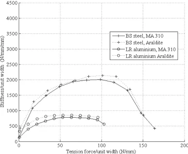
Whilst it might reasonably be expected that joints using an adhesive with a higher modulus of elasticity will be stiffer, our laboratory test and FE results (Figure 23) show this not to be the case. It is also observed from the non-linear analysis curves in Figure 23 that their shapes are very similar. It can therefore be proposed that the loss of stiffness for a tension between 80 to 140 N/mm is not due to the change in adhesive modulus and/or the stress for the onset of yielding (from the true-stress true strain curves in Figure 12). We believe the complex shape of the numerical generated stiffness curves in Figure 23 is primarily due to yielding in the steel adherends and the subsequent development and activation of plastic hinges at the overlap ends.
Using FE analysis the effect of adhesive modulus on joint stiffness was investigated in order to determine a lower limit of modulus for which the stiffness of the benchmark BS steel joint would vary by an acceptable amount (deemed to be < 10%). Unfortunately, non-linear true stress-true strain curves for adhesive materials are not ‘easy to come by’ and so an analysis using geometric non-linearity and non-linear adherend material properties was performed, with the adhesive modulus of elasticity constant and in the range 0.1 to 50 GPa. Figure 24 reports the predicted stiffness response using results of a FE analysis reported in [19]. The gradient of the stiffness curve for values of adhesive modulus between 5 and 50 GPa is shown as a solid line. The ‘dot dash’ line depicts a 5% decrease in this stiffness whilst the dotted line is for a 10% decrease. The inset plot for modulus to 1 GPa shows that, for the benchmark joint geometry, the stiffness will vary by < 5%, or < 10%, when the modulus range is from 0.46 GPa to 50 GPa, or is from 0.32 to 50 GPa, respectively. The two adhesives (MA 310 and Araldite) used in the series of laboratory tests have an initial modulus of elasticity of 2.1 and 2.9 GPa. This 38% difference in modulus is found to produce < 4% difference in joint stiffness when compared to the joint stiffness value on assuming the adhesive modulus is ‘rigid’ (i.e. it is 50 GPa).
GPa, and if the allowed stiffness change can be halved to 5% the lower limit increases to 0.46 GPa. Consequently, it can be concluded that the use of a ‘high’ modulus adhesive will not produce an increase in joint stiffness. Furthermore, the loss of modulus due to the development of adhesive plasticity will never cause the current (mean) modulus of the adhesive layer to fall below the minimum threshold value.
By increasing ta to 3.0 mm, FE analysis demonstrates that the joint stiffness will decrease but the threshold is insensitive to change in the adhesive thickness.
Accordingly, for the purpose of FE modelling of lap-joints, the adhesive can be represented as a linear elastic material and the modulus of elasticity can be assigned any value that exceeds a minimum, This minimum is found to depend on joint geometry; for the benchmark joint geometry and BS steel adherends it is 0.46 or 0.32 GPa for a numerical stiffness difference from that calculated with a ‘rigid’ adhesive joint of 5% or 10%, respectively.
Because a bond line thickness, ta, of 0.3 mm is commonly specified for standard lap-joint testing it was the ‘benchmark’ adhesive thickness (Table 1). For fabrication of vehicle bodies greater bond line thicknesses, of say 1.5 to 3.0 mm, will be necessary. Plotted in Figure 25 is stiffness with load (P) for four constant values of bond line thickness. Because load path eccentricity and adhesive layer shear flexibility are dependent on ta the joint is stiffer the thinner is the bond line. The plots also show that predicted stiffness is always much higher from the non-linear analysis and that the rate of change increases as adhesive thickness gets smaller. The five fold increase when reducing ta from 1.6 mm to 0.3 mm shows that this key parameter has a significant influence on how the joint stiffness changes with tension loading. Adhesive thickness must be included in the simplified shell element model of Part 2 [6].
parameters in establishing the stiffness and strength of tension loaded bonded single lap-joints.
To evaluate the effects of each individual key parameter in Table 1 the percentage increase from the benchmark steel joint value is plotted in Figure 26 against the percentage change in stiffness. The FE results in this figure are for the single load of P = 800 N (or 32 N/mm). As already mentioned the benchmark ta is 0.3 mm, as this value corresponds with the usual coupon requirement for laboratory testing to characterise such lap-joints. This ta is too low for vehicle body construction and so the 100% stiffness in Figure 26 is for an assumed manufacturer’s adhesive thickness of 1.6 mm. To obtain a 90% reduction in stiffness an extrapolation of the ta curve in Figure 26 suggests that the new bond line will need to be 4.8 mm thick. Based on the information given by the four curves in Figure 26 it would be advisable to increase adherend thickness (t1) to achieve the most rapid increase in joint stiffness, if only one key parameter is to be modified. Reducing ta, or increasing adherend modulus of elasticity (Mah), is seen to produce similar stiffness changes. Interestingly, three of the four curves tend towards a horizontal plateau and this would indicate that there is a limit to the usefulness of further increasing adhesive thickness (ta), adherend modulus of elasticity (Mah) and the overlap length (l).
Variations in joint stiffness with tensile loading have been shown in this paper to be dominated by the properties of the adherends and their deformations opposing the decreasing secondary moment from the presence of a load path eccentricity. To ensure that any simplified model in Part 2 can account for the physical characteristics of real single lap-joints the FE analysis must involve, as previously shown by work in reference [11], material non-linearity of the metal adherends. For the reasons developed above the adhesive material can be assumed to have a linear elastic response as we are not concerned with the need to determine the failure load when the adhesive bond ruptures. To be able to capture the complex non-linear shape of a joint’s stiffness (see Figures 5 to 10) it is essential for the FE analysis to account for geometric non-linearity.
CONCLUSIONS
10 specimens, and by changing key parameters to joint design. Computational results from a solid finite element model of the lap-joints with a refined mesh (163k degrees of freedom for the benchmark joint having width of 25 mm) are evaluated against the test curves. The ANSYS finite element code was used for the combined material (adherends only) and geometric non-linear analysis for computing joint stiffness. The comparison is found to be very good over the full non-linear load-displacement response, although the finite element analysis does not give the failure load when the adhesive ruptures. Because the refined solid model requires excessive computing resources a trial and error approach is used to minimise the number of degree of freedom (< 10k) in a solid element mesh, whilst at the same time maintaining adequate numerical predictions when assessed against real non-linear joint deformations. This modelling exercise produces a coarse solid element mesh that requires 1/5th of the run time of the original solid element mesh and thereby enabled the authors to conduct a finite element parametric study for the sensitivity of changes to the seven key design parameters.
be unable to include the actual deformation response of bonded single lap-joints in whole vehicle analyses.
[image:22.612.101.513.376.494.2]Table 1. Values of parameters for laboratory testing of single lap-joints Figure 2).
Table 2. Linear elastic properties for the adhesive materials in FE analysis.
ESP 105 Araldite MA 310 F 241
Modulus of elasticity
(GPa) 5.8 2.9 2.1 0.85
Strain at limit of elasticity
(strain) 0.048 0.009 0.01 0.006
Stress at limit of elasticity
(MPa) 26.1 25.1 25.7 3.7
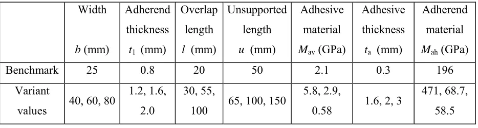
Table 3. Lap-joint parameter values for FE analysis. Width
b (mm)
Adherend thickness t1 (mm)
Overlap length l (mm)
Unsupported length u (mm)
Adhesive material Mav (GPa)
Adhesive thickness ta (mm)
Adherend material Mah (GPa)
Benchmark 25 0.8 20 50 2.1 0.3 196
Variant
values 40, 60, 80
1.2, 1.6, 2.0
30, 55,
100 65, 100, 150
5.8, 2.9,
0.58 1.6, 2, 3
471, 68.7, 58.5 Width b (mm) Adherend thickness t1 (mm)
Overlap length l (mm)
Unsupported length u (mm)
Adhesive material
Mav
Adhesive thickness ta (mm)
Benchmark 25
0.8 for steel 1.2 for aluminium
20 50 MA 310 0.3
Variant
[image:22.612.90.557.547.672.2]REFERENCES
[1] United States Code 49, Subtitle VI, Motor Vehicle and Driver Programs, Part C. Information, Standards, and Requirements, Chapter 329. Automobile Fuel Economy. 2003
[2] C. Carraro, D. Siniscalco, The European Carbon Tax: An Economic Assessment. Kluwer Academic (Pub). ISBN 0792325206 (2000).
[3] A.H. Lundgren, Volvo Laboratory Study of Zinc-Coated Sheet Steel - Adhesive Bonding Properties. SAE Technical Paper, Sect 5, 890703 (1989) 613-618.
[4] L. J. Hart-Smith, Designing To Minimise Peel Stresses In adhesive Bonded Joints. McDonnel Douglas Report 7389 (1983)
[5] L. F. M. da Silva, R. Carbas, G. Critchlow, M. Figueiredo, K. Brown, Effect of Material, Geometry, Surface Treatment and Environment on the Shear Strength of Single Lap Joints. Int J Adh Adh 29 (2009) 621-632.
[6] I. T. Pearson, J.T. Mottram, A Modelling Methodology for the inclusion of Bonded Lap-joints in the Finite Element Analysis of Automobile Bodies: Part 2 – Novel shell mesh to minimise analysis time. Submitted to Computers and Structures.
[7] R. Andruet, D. Dillard, S. Holzer, Two- and Three-Dimensional Geometrical Nonlinear Finite Elements for Analysis of Adhesive Joints. Int J Adh Adh, 21 (2001) 17–34. [8] J. Concalves, M. Moura, P. Castro, A Three-Dimensional Finite Element Model for
Stress Analysis of Adhesive Joints. International Journal of Adhesion and Adhesives, 22 (2002) 357–65.
[9] U. Edlund, Surface Adhesive Joint Description With Coupled Elastic–Plastic Damage Behaviour and Numerical Applications. Computer Methods in Applied Mechanical Engineering 115 (1994) 253–276.
[10] D. Castagnetti, E. Dragoni, A. Spaggiari, Efficient Post-Elastic Analysis of Bonded Joints by Standard Finite Element Techniques. Journal of Adhesion Science and Technology, 23, 10-11 (2009) 1459-1476.
[11] U. Edlund, P. Schmidt, E. Roguet, A Model of an Adhesively Bonded Joint with Elastic-plastic Adherends and a Softening Adhesive. Comput Method Appl M, 198 (2009) 740-752.
[13] G. Li, P. Lee-Sullivan, R. W. Thring, Nonlinear Finite Element Analysis of Stress and Strain Distributions across the Adhesive Thickness in Composite Single-Lap Joints. Compos Struct, 46(4) (Dec 1999) 395-403.
[14] L. Goglio, M. Rossetto, Stress Intensity Factor in Bonded Joints; Influence of the Geometry, Int J Adh Adh, 30, 2010, pp313-321.
[15] R. Adams, J. A. Harris, The influence of local geometry on the strength of adhesive joints. Int J Adh Adh, 7(2) (April 1987) 69-81.
[16] M. Goland, E. Reissner, The Stresses in Cemented Joints. J Appl Mech, Trans ASME, 66 (1944) A17-A27.
[17] L. J. Hart-Smith, Adhesive Bonded Single Lap Joints. NASA Technical Report CR-112236. 1973.
[18] L. J. Hart-Smith, Further Developments in the Design & analysis of adhesive-Bonded Structural Joints, NASA CR-112235, 1973.
[19] I. T. Pearson, A Method for the Inclusion of Adhesively Bonded Joints in the Finite Element Analysis of Automobile Structures, PhD thesis, School of Engineering, University of Warwick, 2006.
[20] T. Wang, O. Hopperstad, P. Larsen, O. Lademo, Evaluation of a Finite Element Modelling Approach for Welded Aluminium Structures. WIT Transactions for Engineering Science, V49. ISSN 1743-3533. WIT Press 2005
[21] The Automotive Steel Design Manual. Available from the WWW at http://www.a-sp.org/database/pdf/CarsAsdm/Chapter2/section2-05.pdf. Last viewed 17 April 2011 [22] G. D. Dean, F. Hu, B. C. Duncan, The Application of Finite Element Methods to the
Design of Adhesive Joints, MTS Adhesive Project 1. Report N3 May 1995.
[23] A. D. Crocombe, D. A. Bigwood, Analysing Structural Adhesive Joints for Failure. Int J Adh Adh, V10 N3 July 1990.
[24] G. D. Dean, B. C. Duncan, Tensile Behaviour of Bulk Specimens of Adhesives, MTS Adhesive Project 1. Report N3 May 1995.
[25] J. T. Mottram, C. T. Shaw, Using Finite Elements in Mechanical Design, McGraw-Hill, Maidenhead, 1996.
[26] L. Grant, R. Adams, L. da Silva, Experimental and Numerical Analysis of Single-lap Joints for the automotive industry. Int J Adh Adh 29 (2009) 405-413.
[28] M. Abou-Handa, M. Megahed, M. Hammouda, Fatigue Crack growth in double Cantilever Beam Specimen with an Adhesive Layer. Eng Fract Mech, 60 (1998) 605-614.
[29] L. Kawashita, A. Kinloch, D. Moore, J.T. Williams, The Influence of Bond Line Thickness and Peel Arm Thickness on Adhesive Fracture Toughness Of Rubber Toughened Epoxy–Aluminium Alloy Laminates. Int Journal Adh Adh, 28 (2008) 199– 210.
[30] R. Kahramana, M. Sunarb, B. Yilbas, Influence of Adhesive Thickness And Filler Content on The Mechanical Performance of Aluminum Single-Lap Joints Bonded With Aluminum Powder Filled Epoxy Adhesive. J Mater Process Tech, 205 (2008) 183–9. [31] A. Neves, E. Coutinho, A. Poitevin, J. Van der Sloten, B. Van Meerbeek, H. Van
Oosterwyck, Influence of Joint Component Mechanical Properties and Adhesive Layer Thickness on Stress Distribution in Micro-Tensile Bond Strength Specimens. Dent Mater 25 (2009) 4–12.
Figure captions
Figure 1. Bonded joint configurations: (a) coach joint; (b) single lap-joint. Figure 2. Key joint parameters influencing stiffness response.
Figure 3. Test specimens for the three overlap lengths and two extensometer gauge lengths. Figure 4. Axial displacement measurement using the Messphysik video extensometer. Figure 5. Stiffness of lap-joints having three different joint widths, b.
Figure 6. Stiffness of aluminium lap-joints with two adherend thicknesses, t1.
Figure 7. Stiffness for aluminium lap-joints (ta = 1.2 mm) with change in overlap length, l. Figure 8. Stiffness of steel and aluminium lap-joints with change in the unsupported length,
u.
Figure 9. Stiffness of steel and aluminium benchmark lap-joints with change in adhesive material, Mav.
Figure 10. Stiffness of steel and aluminium lap-joints with change in adhesive thickness, ta. Figure 11. True stress/strain relationships for four metallic adherend materials.
Figure 12. True stress/strain relationships for four adhesive materials.
Figure 13. Half benchmark lap-joint model showing a very refined solid element mesh and its refinement of 14 elements through thickness at an overlap end.
Figure 14. Half benchmark lap-joint model showing the coarser solid element mesh and the 8 elements through thickness at an overlap end.
Figure 15. Comparison of FE results and test tension load with axial displacement for the steel and aluminium benchmark lap-joints.
Figure 16. Comparison of FEA and measured mean stiffness by testing for the benchmark steel lap-joint.
Figure 17. Joint stiffness for BS steel lap-joints of different joint widths, b, from 25 to 80 mm.
Figure 18. Joint stiffness for BS steel lap-joints with change in adherend thickness, ta, from 0.8 to2.0mm.
Figure 19. Joint stiffness for four adherend materials, Mah.
Figure 20. Joint stiffness for BS steel lap-joints with change in overlap, l, from 20 to 100 mm.
Figure 22. Joint Stiffness for BS steel lap-joints with change in unsupported length, u, from 50 to 150 mm.
Figure 23. Joint stiffness for BS steel lap-joints for four different adhesive materials, Mav. Figure 24. Influence of changing the adhesive’s modulus of elasticity from 0 to 10 GPa on
stiffness on BS steel lap-joint with benchmark geometry.
Figure 25. Joint stiffness of BS steel lap-joints with change in adhesive thickness, ta, from 0.3 to 3 mm.
Figure 1
(a) (b)
P
P P
Figure 2
Adhesive material (Mav)
Adherend thickness (t1)
Overlap length (l)
Adhesive thickness (ta)
Unsupported length (u)
Width (b)
P P