Emmanuel FR ´ENOD, Emmanuel MAITRE, Antoine ROUSSEAU, St´ephanie SALMON and Marcela SZOPOS Editors
A MIXTURE MODEL FOR THE DYNAMIC OF THE GUT MUCUS LAYER
Tamara El Bouti
1, Thierry Goudon
2, Simon Labarthe
3, B´
eatrice Laroche
3,
Bastien Polizzi
2, Amira Rachah
4, Magali Ribot
5 2and R´
emi Tesson
6Abstract. We introduce a mixture model intended to describe the dynamics of the mucus layer that wraps the gut mucosa. This model takes into account the fluid mechanics of the gut content, the inhomogeneous rheology that depends on the fluid composition, and the main physiological mechanisms that ensure the homoeostasis of the mucus layer. Numerical simulations, based on a finite volume approach, prove the ability of the model to produce a stable steady-state mucus layer. We also perform a sensitivity analysis by using a meta-model based on polynomial chaos in order to identify the main parameters impacting the shape of the mucus layer. The effect of the interaction of the mucus with a population of bacteria is eventually discussed.
R´esum´e. Nous pr´esentons un mod`ele de m´elange qui d´ecrit l’´evolution de la couche de mucus qui recouvre la muqueuse du gros intestin. Ce mod`ele prend en compte la m´ecanique des fluides qui composent le contenu intestinal, la rh´eologie inhomog`ene d´ependant de la composition du fluide et les principaux m´ecanismes physiologiques qui assurent l’hom´eostasie de la couche de mucus. Des r´esultats num´eriques, obtenus par une m´ethode volumes finis, d´emontrent la capacit´e du mod`ele `a reproduire une couche de mucus stationnaire stable. Nous pratiquons ensuite une analyse de sensibilit´e en construisant un m´etamod`ele bas´e sur des polynˆomes de chaos afin d’identifier les param`etres impactant le plus la forme de la couche de mucus. Finalement, nous discutons les effets des interactions entre la couche de mucus et une population bact´erienne chimiotactique.
1.
Introduction
The distal human gut, also known as colon, is inhabited by a complex microbial ecosystem, the gut microbiota. Recent progresses in the knowledge of the microbiota structure and function have demonstrated its direct or indirect implication in various affections, among which Crohn’s disease, allergic and metabolic disorders, obesity, cholesterol or possibly autistic disorders. Understanding the gut microbiota ecology is one of the current scientific hot-spot in microbiology. The gut microbiota provides to his human host several benefits, such as energy harvesting [20], barrier function against pathogens and immune system maturation [21]. However, even these beneficial commensal bacteria represent an infection threat for the host. Alongside with complex active immune mechanisms, a first simple and passive protection is an insulating layer of mucus that physically separates the microbial populations from the host tissues.
1 Universit´e Versailles St-Quentin, CNRS, UMR 8100 Labo. de Math´ematiques de Versailles 2 Universit´e Cˆote d’Azur, Inria, CNRS, LJAD
3 MaIAGE, INRA, Universit´e Paris-Saclay, 78350 Jouy-en-Josas, France
4 Universit´e Toulouse 3, CNRS, UMR 5219 Institut de Math´ematiques de Toulouse 5 On leave to Universit´e d’Orl´eans, CNRS, UMR 7349 MAPMO
6 Aix–Marseille Universit´e, CNRS, UMR 7373 Institut de Math´ematiques de Marseille
c
EDP Sciences, SMAI 2017
This mucus barrier is actually composed of two distinct layers with different rheological characteristics. A first viscous layer wraps the epithelial cells. An external, thicker and more fluid layer covers the first one [13]. These rheological discrepancies are attributed to structural differences in the mucus protein folding and to hydration/dehydration effects. The active water pumping of the intestinal mucosa dries out the inner layer of mucus, whereas the liquid luminal content keeps the outer layer hydrated. Mucus turn over results from the erosion of the external layer by the luminal flux and the continuous renewal of the inner layer by the mucosa [23]. Unlike the inner layer, the outer layer can be penetrated by bacteria, which thereby take advantage of this food source, resist the luminal flow and increase their residence time in the gut. It represents an ecological niche that influences the global equilibrium of the gut microbiota. A good model of its dynamics is then a key issue in the perspective of constructing accurate models of the gut microbiota ecology. This modelling work could help physiologists and microbiologists to better describe and understand the main parameters in mucus layer formation or disruption and to study host-microbiota interactions and microbiota ecology in an integrative way. Since there is no sharp interface between the mucus and the luminal liquid, our approach adopts the mixture flows framework. Further details about the mixture theory can be found in [19, 24]. It leads to systems of Partial Differential Equations (PDE) describing a mixture of several components with different physical properties. For adaptation of mixture theory for describing biological flows, we refer the reader to [14] (poro-elastic materials), [18] (tumor growth), and [6] (growth of phototrophic biofilms). The formation of layers of biological mucus can also be described at the molecular scale [11]. A compartmental model, written in terms of a large set of Ordinary Differential Equations describing fibre degradation by gut microbial populations, has been proposed in [16]. In this 0D model, the mucus is modelled as a separate compartment but spatial mechanisms are loosely described and the underlying fluid mechanics is discarded. A model based on the principles of fluid mechanics for pulmonary mucus appeared in [5]; it describes mucus evacuation by cilla without investigating the dynamics of the mucus layer formation. To our knowledge, the present work is the first attempt of a fluid mechanics model specially designed to describe the intestinal fluid flows involved in the constitution of the ecological environment of the gut microbiota. Together with adapted population dynamics and host response models, it constitutes a key component of a global ecological model of intestinal microbial communities.
We organize the article as follows. We introduce the mixture model of intestinal fluid flow in Section 2. Section 3 focuses on the boundary conditions and sketches the derivation of an approximate model. Section 4 details the numerical method used for the simulation of the model and test cases are presented in Section 5. We analyse the sensitivity of the approximate model in Section 6. Finally, we extend the model by including a chemotactic bacterial population in the mixture model in Section 7.
2.
A mixture model for the fluid dynamics in the human gut
2.1.
Mathematical modelling of the gut content
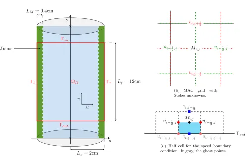
A schematic view of the gut, which makes the length scales precise, is represented on Fig. 1a; the mucus layer (in green) measures about four millimeters. In what follows, the geometry is drastically simplified and curvature effects are neglected: we will simply work on a 2D rectangular domain ΩD, delimited by two lateral
boundaries Γl(x=−Lx),Γr(x=Lx), that represent the gut mucosa, the superior boundary Γin(y = 0) and
the inferior boundary Γout(y=−Ly) which stand respectively for the inflow and outflow boundaries.
We assume in this model that the gut content is a mixture of two components: the mucus and the luminal content. LetM(t, X) andL(t, X) be the volume fractions, at timet >0 and positionX = (x, y)∈ΩD, occupied
by the mucus and the liquid luminal phase, respectively. We then have, for allt andX
M(t, X) +L(t, X) = 1. (1)
ESAIM: PROCEEDINGS AND SURVEYS 113
x y
Ly= 12cm
u v
Lx= 2cm
LM '0.4cm
Mucus Γl Γin Γr Γout ΩD
(a)Representative view of the gut
Pi−1,j−1 Pi,j−1 Pi+1,j−1
Pi−1,j Mi,j Pi+1,j
Pi−1,j+1 Pi,j+1 Pi+1,j+1
ui−3
2,j−1 ui−
1
2,j−1 ui+
1
2,j−1 ui+
3 2,j−1 ui−3
2,j ui−
1
2,j ui+
1
2,j ui+
3 2,j ui−3
2,j+1 ui−
1
2,j+1 ui+
1
2,j+1 ui+
3 2,j+1
vi−1,j−3 2
vi−1,j−1 2
vi−1,j+1 2
vi,j−3 2
vi,j−1 2
vi,j+1 2
vi+1,j−3 2
vi+1,j−1 2
vi+1,j+1 2
(b) MAC grid with
Stokes unknowns.
Mi,j
ui−1
2,j ui+
1 2,j
ui−1
2,j−12 vi,j−12 ui+12,j−12
vi,j+1 2
Γout
(c) Half cell for the speed boundary condition. In gray, the ghost points.
Figure 1. Computation domain and illustration of the MAC discretization — See Section 4.
DL) the diffusion coefficient for M (resp. L). The mass conservation equations then read
∂tM +∇X·(M V −DM∇XM) = 0, (2)
∂tL+∇X·(LV −DL∇XL) = 0. (3)
The velocity field (t, X)7→V(t, X) is determined using fluid mechanics principles. Since the Reynolds number is low, we neglect convective effects and we use the Stokes equations. The velocity is solution of
−∇X· µ(M) ∇XV +∇XVT+∇XP = 0 (4)
whereµ(M) is the viscosity andP is the hydrostatic pressure. The viscosity is a function of the mucus volume fraction, bearing in mind that µis much larger in the mucus than in the fluid. Summing Eq. (2) and (3), and using Eq. (1), we are led to the following constraint
∇X·V =∇X·((DM−DL)∇XM). (5)
In order to detail the modeling assumption, it is convenient to introduce the velocity fields
Then the continuity equations can be rewritten in the more conventional form
∂tM +∇X·(M uM) = 0 =∂tL+∇X·(LuL)
by means of the constituents’ velocitiesuM anduL. The constraint (5) traduces the fact that the mean volume
velocityM uM+LuLis solenoidal. Eq. (6) is a constitutive law, it has the form of a Fick’s law for the relative
velocities uM −V and uL−V, derived from the principles of mixture theory [19, 24], in order to define the
effective velocity V of the mixture. The role of the diffusion coefficients DM, DL >0 is precisely to make the
mixture more homogeneous by imposing mass transfer by diffusion. Note that the bulk velocity is divergence free when the mixture is made of one constituent only (M = 0 orM = 1); otherwise compressibility is driven by the difference DM−DL.
For the continuous equations, we can work equivalently with (1), (2), (3), (4) or (1), (2), (4), (5). We complete the system by an initial conditionMt=0=M0 and boundary conditions on∂Ω, that will be detailed
later on.
Remark 2.1. Since in general ∇X·V 6= 0, it could be relevant to add in the Stokes equation (4) the term ∇X(λ∇X·V)) with a viscosity coefficientλ≥0 that is required to satisfy some compatibility relation withµ.
Here, we simply setλ= 0, which is always admissible.
2.2.
Parameter settings
Our model involves several quantities having typical front-like behavior, that we model with sigmoidal func-tions. We set
Σ+P(x) = (pmax−pmin)
x2αp
x2αp+χ2pαp
+pmin and Σ−P(x) = (pmax−pmin)
1− x
2αp
x2αp+χ2pαp
+pmin (7)
which depend on a set of 4 parameters embodied into the shorthand notationP = (pmax, pmin, αp, χp). We see
that Σ+ (resp. Σ−) is an increasing (resp. decreasing) sigmoidal function with limit valuesp
min < pmax,χp is
the inflexion point andαp modulates the transition slope.
Firstly, let us discuss the form of the viscosity distribution. We suppose that the mucus is more viscous than the luminal content and that there exists a concentration threshold that completely changes the rheological properties of the fluid. We then model the function µwith the parametersPµ= (µmax, µmin, αµ, χµ) and the
sigmoidal function
µ(M)(x, y) = Σ+P
µ(M(x, y)).
Secondly, we focus on the diffusion coefficientsDM andDL. Those diffusion coefficients may depend on the
local composition of the mixture, but are also strongly determined by spatial features, such as the microscopic structure of the mucus gel and of the gut wall. In order to avoid additional non linearities and regarding the lack of precise knowledge of the links between mucus concentration, mucus layer microscopic structure and effective diffusion, we chose to only consider spatial dependence of the diffusion by introducing specific modelling assumptions. Some perspectives to improve the model on that issue will be given in the last section We suppose that the mucus layer is confined near the mucosa. Consequently, the correction tuned byDM should be small
near Γl∪Γr and high at the center of the domain, and reversely forDL. We also suppose thatDM andDL are
uniform with respect toy. DenotingPK= (DK,max, DK,min, αK, χK) withK∈ {L, M}, we set
DL(x, y) = Σ+PL(x) and DM(x, y) = Σ−PM(x).
Thirdly, we assume that the mucus is initially essentially located near the mucosa with a sharp transition; givenPM0 = (M0,max, M0,min, αM0, χM0), it leads to define
M0(x, y) = Σ+PM
3.
Discussion on the boundary conditions
We face different modelling issues concerning boundary conditions. We remind the reader that the different boundaries of the domain describe completely different physiological functions. On the one hand, the lateral boundaries Γl∪Γrrepresent the intestinal mucosa which produces mucus and pumps luminal liquid, influencing
both mass conservation and flow speeds. On the other hand, the horizontal boundary conditions on Γin and
Γout have to model free inflow and outflow of matter.
3.1.
Boundary conditions for
Γ
l∪
Γ
rOn the lateral boundaries, the flux is driven by mucus production and liquid pumping according to
(M V −DM∇XM)·~n=−fM(M) and (LV −DL∇XL)·n~ =−fL(L), (9)
Mucus production and water pumping depend on certain thresholds: we set
fM(M) =θM[M−M∗]−, fL(L) =−θL[L−L∗]+.
The former means that the mucosa produces at rateθM when the mucus concentration is below the threshold
M∗, while the latter tells us that the mucosa pumps liquid at rateθLonly when the liquid concentration is above
the thresholdL∗. A linear combination of (9), together with (1), yields
M+DM DLL
V ·~n=−fM −DDLMfL. It
implies a Dirichlet boundary condition for the transverse velocityu. We can freely definev on Γl∪Γrwithout
influencing the normal flow ofM andL. Keeping in mind compatibility conditions at the corners of the domain, we impose that the tangential velocity vanishes. We arrive at
V ·~n=u=−fM+
DM DLfL
M+DMDLL and V ·~τ=v= 0. (10)
3.2.
Boundary conditions for
Γ
inand
Γ
outThe definition of relevant boundary conditions on Γinand Γoutis more challenging. We assume that diffusion
does not contribute to fluxes at the inflow and outflow boundaries:
DM∇XM ·~n= 0 and DL∇XL·~n= 0. (11)
The boundary conditions for the velocity have a crucial role on the behaviour of the model: by constraining the velocity field, they drive the mucus displacement and its equilibrium with the liquid inside the domain. The boundary conditions should produce a stable mucus layer without over constraining the system in a non physiological way. Choosing Dirichlet boundary conditions at Γinis relevant since the average fluid intake into
the gut is a known biological parameter. As the intestinal flow is mainly longitudinal, it might be natural, at first sight, to assume that the transverse velocity is null on this boundary. On the contrary, relaxing the constraint on Γoutis meaningful because we want to investigate the model response to the inflow only. For that
reason, we choose a no-strain boundary condition. We then get
u= 0 and v=vin on Γin and µ(M) ∇XV +∇XVT
−P Id~n= 0 on Γout (12)
Remark 3.1. The numerical simulations in Section 5.1 show that the no-strain condition on Γoutcould produce
questionable velocity and mucus distribution profiles in the vicinity of Γout, likely due to the use of the symmetric
3.3.
Derivation of an approximated profile for
v
in.
We wish to capture steady–states with mucus layers next to the lateral boundaries. Accordingly, since the viscosity µhas a sharp profile as a function ofM, strong variations of the velocity are expected in this region too. The boundary conditions on Γinshould reflect this behavior in order to avoid too strong correction of the
velocity field near Γin. We will discuss several options to obtain such a relevant profile for (uin, vin), compatible
with the expected steady–states. One of them consists in deriving an approximation of the inflow.
To this end, we find a reduced model based on asymptotic reasoning. We rewrite the equations in dimen-sionless form and we make the aspect ratioε= LxL
y appear. It turns out that the regime 0< ε1 is relevant
for our purposes. We seek solutions as an expansion in power series ofε, where for the velocity the leading term has the form (εu1, v0). A specific regime of the pressure characteristic value leads to an explicit formulation
of v0, which links the velocity with the viscosity distribution and the boundary conditions. As we specifically
focus on the case of a sharp mucus layer located near the mucosa in the vicinity of Γin, we approximate the
corresponding viscosity profile with the step function ˜µ=µmin1(0,Rm)+µmax1(Rm,1)for a certain 0< Rm<1
(in dimensionless units). We introduce ˜µ in the explicit formulation of v0, which gives the following formal
approximation for the longitudinal velocity on Γin
vin(x) =
win
γ 1
−x2
2µmax
1(Rm,1)(x) + 1
−R2
m
2µmax
+R
2
m−x2
2µmin
1(0,Rm)(x)
, (13)
where
γ= 1 8
1
µmin
R4m+ 1
µmax
(1−R4m)
,
with given win>0, 0< Rm<1. The simplified asymptotic model of the flow (i.e. (εu1, v0)) will be used for
the sensitivity analysis in Section 6 since it permits us to reduce the computational cost.
4.
Numerical scheme
We update the mucus volume fraction with (2), the velocity-pressure pair is determined by the system (4)– (5) while the luminal liquid volume fraction L is simply defined by (1). We choose a semi-implicit scheme so that the computation of the volume fractions and the velocity–pressure fields are decoupled. We work with Cartesian grids and we use well-established schemes for both equations. The diffusion term in (2) is treated by the VF4 method, which is known to converge on meshes satisfying the orthogonality condition, such as Cartesian grids [9, Sect. 3.1.1]. The transport term is approached according to UpWind principles. The Stokes system is dealt with by using the MAC scheme, which dates back to [12]. Accordingly, pressure, horizontal, and vertical velocities are evaluated on staggered grids; the volume fractionM is stored on the same grid as the pressure, see Fig. 1b. We refer to the grid cells and the corresponding unknowns with the notations Ωi,j (for
P,M grid), Ωi−1
2,j (foru) and Ωi,j−12 (forv).
The Finite Volume framework mimics the formulae obtained by integrating the equations over the grid cells. For instance, for the horizontal velocity we get
Z
∂Ωi−1 2,j
µ(M) ∇XV +∇XVT·~n dω− Z
Ωi−1 2,j
∂xP dΩ = 0 (14)
where~nis a outward normal vector to the boundary of Ωi−1
2,j. The boundary integral splits as a sum over the
to the following discrete equivalent to (14)
−∆xµ˜i−1 2,j−12
−ui−1/2,j−∆uyi−1/2,j−1 −vi,j−1/2−∆vxi−1,j−1/2
−∆y µ(Mi,j)
2ui+1/2,j−ui−1/2,j ∆x
−∆xµ˜i−1 2,j+
1 2
u
i−1/2,j+1−ui−1/2,j
∆y +
vi,j+1/2−vi−1,j+1/2
∆x
+ ∆y µ(Mi−1,j)
2ui−1/2,j −ui−3/2,j ∆x
+ ∆x∆yPi,j−Pi−1,j
∆x = 0.
(15) The quantities ˜µare not directly defined sinceM, and thusµ, is not stored at the interfacesi+12, j+12, where it needs to be reconstructed. For instance we can use the mean value ˜Mi+1
2,j+ 1 2 =
1
4(Mi,j+Mi,j+1+Mi+1,j+
Mi+1,j+1). When the viscosity has a sharp profile, it can be more efficient to reconstruct ˜µi+1 2,j+
1
2 by the
harmonic mean [9, Sect. 2.3]. We proceed similarly with the vertical velocity, integrating the second component of Eq. (4) . Finally integrating (5) over Ωi,j leads to
∆x(vi,j+1/2−vi,j−1/2) + ∆y (ui+1/2,j−ui−1/2,j) =Di,j (16)
whereDi,jis the approximation of the diffusion flux R
∂Ωi,j(DM−DL)∇XM·~n dωdefined by the VF4 formalism
[9]. The same numerical flux is used to updateM through the discretization of (2) where the convection term is obtained with explicit upwind fluxes, while the diffusion term is treated implicitly.
The boundary conditions are discretized differently according to the boundary and the equation under con-sideration. The convection–diffusion equation for M is complemented either by the Robin condition (9), with a convection flux given on Γr, Γl by (10), or the Neumann condition (11) on Γin, Γout with a convection flux
given by (12).
On the boundaries Γl, Γr (resp. Γin), the treatment of the equations involving non–interior values foru, v
andM is rather standard. The velocities are determined by using the Dirichlet boundary condition (10), while for the volume fraction we use the Robin-like (resp. Neumann) condition in (9) (resp. (11)) to define the missing
M’s.
On Γout the viscous fluxes vanish by virtue of (12) . The diffusion fluxes for M are also set to 0 due to
(11). The only difficulty comes when evaluating the vertical velocity. To this end, we integrate the second component of Eq. (4) in half a grid cell and we introduce ghost points, as shown in Fig. 1c. We observe that three contributions on the boundaries of the cell vanish thanks to the boundary condition (12); the forth boundary on the top gives an equation forv on such boundary cells Ωi,j−1/2.
5.
Numerical results
For the numerical experiments, the computational domain is ΩD= [−Lx, Lx]×[−Ly,0], withLx= 2,Ly= 12
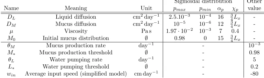
(incm) and we work with 100×300 grid points that define square cells. The parameters of the model are given in Table 1. We shall comment the role of the conditions on Γin and Γout and discuss numerical experiments
where a stable mucus layer establishes.
5.1.
Comments on the boundary conditions
As explained in Remark 3.1, it is likely that the velocity imposed on Γinplays a crucial role in the formation
of the mucus layer, and a certain compatibility should be satisfied between the expected steady state and the incoming field (uin, vin). If no measurements are available, we can start with the profile (13) (anduin = 0)
which is based on an asymptotic argument. According to the intuition, the velocity field is quite uniform in the vertical direction, see Fig. 3a for an overview of the horizontal speed over the whole domain. It suggests that the condition on Γin can be improved with the following iterative procedure: a) Define (u, v) by solving the
system (4)–(5), b) set (uin, vin)(x) = (u, v)(x,− Ly
Sigmoidal distribution Other Name Meaning Unit pmax pmin αp χp value
DL Liquid diffusion cm2day−1 2.5.10−3 10−4 16 34Lx
-DM Mucus diffusion cm2day−1 10−5 10−6 12 34Lx
-µ Viscosity Pa s 1.97·10−2 10−3 7 0.4
-M0 Initial mucus distribution ∅ 0.98 0 15 34Lx
-θM Mucus production rate day−1 - 10−3
M∗ Mucus production threshold ∅ - 0.98
θL Water pumping rate day−1 - 5
L∗ Water pumping threshold ∅ - 0.2
win Average input speed (simplified model) cm day−1 - -80
Table 1. Biophysical constants of the model. Sigmoidal distribution is defined with Eq. (7).
The parameters pmax and pmin are the maximal and minimal bounds of the sigmoid, αp its
slope and χp its inflexion point. We emphasize that the diffusion parameters for the liquid
and the mucus are respectively of order 10−12m2s−1 and 10−14m2s−1, in order to mimic the
diffusion of large molecules —such as polysaccharides— in highly viscous media — such as the chyme and the mucus. They remain in documented orders of magnitude for large molecule diffusions in mucus [15].
by the fact that we are only considering a relatively short portion of the gut. Note that we have two choices foruin thereafter, namely we can setuin= 0 as before or we can use the functionuingiven as a result of the
iterative procedure.
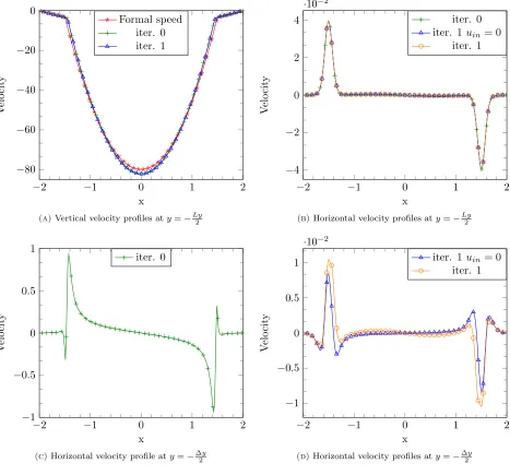
Fig. 2 compares the velocity profiles with 0 or 1 iteration of the iterative procedure aty =−Ly2 , far away from Γin so that the influence of the Dirichlet condition may be moderate, and aty=−∆2y where boundary–
layer effects can be sensitive. We pay a specific attention to the role of uin. As far as we consider the vertical
component v of the velocity, the resulting profiles are quite similar between two consecutive iterations of the iterative procedure, and quite close to the formal approximation given by Eq. (13) (the maximal relative difference is 5%) including next to Γin, see Fig. 2a. Conversely, if we use an alternative iteration procedure to
definevin only, but keepinguin= 0, very slight discrepancies are observed onuat−Ly/2, but boundary–layer
effects are clearly sensitive next to Γin, see Fig. 2b and 2d : we observe oscillations with high amplitude which
might create instabilities. Those oscillations are two orders of magnitude higher during the iteration 0 than the iteration 1. This discussion reveals that the choice of (uin, vin) is certainly far from harmless.
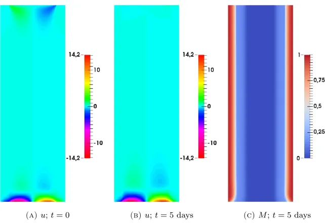
As said in Section 3.2, the condition (12) on Γoutis questionable. We see the effect of the boundary condition
on Fig. 3: significantly larger horizontal velocities appear in the vicinity of Γout. The spurious velocities are
oriented from the lumen of the gut to the wall. Consequently, a part of the mucus near Γout will be washed-out,
as it can be observed on the mucus profile on Fig. 3c after five days: close to Γout the layer of mucus is smaller
than inside the domain. Nevertheless, the flow is mostly oriented outward and, as confirmed by these results, the effects of the null strain boundary condition remain confined close to the boundary.
5.2.
Stable steady–state mucus layer
In order to evaluate the robustness of the model, we compare the large–time state of the flow when we start from the sigmoidal state (8), here denotedM0,s, or from a Gaussian distribution
M0,g(x, y) =Mmax exp −
(x−Lx)
2
2 Lx
6
2 !
+ exp −(x+Lx)
2
2 Lx
6
2 !!
−2 −1 0 1 2
−80
−60
−40
−20 0
x
V
elo
c
it
y
Formal speed iter. 0 iter. 1
(a)Vertical velocity profiles aty=−Ly
2
−2 −1 0 1 2
−4
−2 0 2 4
·10−2
x
V
elo
cit
y
iter. 0 iter. 1uin= 0
iter. 1
(b)Horizontal velocity profiles aty=−Ly
2
−2 −1 0 1 2
−1
−0.5 0 0.5 1
x
V
elo
cit
y
iter. 0
(c)Horizontal velocity profile aty=−∆y 2
−2 −1 0 1 2
−1
−0.5 0 0.5 1
·10−2
x
V
elo
cit
y
iter. 1uin= 0
iter. 1
(d)Horizontal velocity profiles aty=−∆y 2
Figure 2. Speed profiles at y = −Ly2 and y = − ∆y
2 for the first iterations of the iterative
procedure defined in Sec. 5.1. The formal speed designates the boundary conditions (13) used for the initialization of the iterative procedure. The notation uin = 0 stands for the result
of the alternative iterative procedure keeping uin = 0. We had to displayed the horizontal
velocity profiles aty=−∆2y for iter.0 and iter.1 on different plots, due to their different order of magnitude.
For both initial conditions, we perform the same simulations, with the boundary condition (13) for vin. After
60 days the two mucus profiles coincide, see Fig. 4b (in the area where the mucus volume fraction is larger than
1
100 the relative difference on the profiles is about 2%). The mucus layer and its shape are thus not strongly
(a)u;t= 0 (b)u;t= 5 days (c)M;t= 5 days
Figure 3. Horizontal speed uand mucusM distributions att= 0 ort= 5.
to computevin, the profilevindepends on the initial data for M and some discrepancies on the mucus profile
at larger times appear; see Fig. 5 for a comparison between the sigmoidal and the Gaussian profiles.
−2 −1 0 1 2
0 0.5 1
x
Mucus
v
olu
m
e
fraction
M0,g
M0,s
(a)Initial mucus profiles
−2 −1 0 1 2
0 0.5 1
x
Mucus
v
ol
ume
fraction
M0,g
M0,s
(b)Mucus profiles after 60 days
Figure 4. Mucus profiles aty=−Ly
2 for initial dataM0,g andM0,s att= 0 andt= 60 days
withvin given by Eq. (13).
We also investigate the ability of the model to recover its steady states when the mucus layer is strongly perturbed at t= 0. We start from the sigmoidal shape M0,s, and we compute the condition on Γin with the
−2 −1 0 1 2 0
0.5 1
x
Mucus
v
olu
m
e
fraction
Mucust= 0 Mucust= 10 Mucust= 20
(a)Initial conditionM0,g
−2 −1 0 1 2
0 0.5 1
x
Mucus
v
ol
ume
fraction
Mucust= 0 Mucust= 10 Mucust= 20
(b)Initial conditionM0,s
Figure 5. Mucus profiles at y=−L2y for initial dataM0,g andM0,s att= 0, 10 and t= 20
days withvin given by the iterative procedure.
one day, a tongue of mucus is transported from uphill and starts to overlay the eroded mucus layer area. The initial disruption is also transported and its downhill part is abraded by the liquid flow. At t = 2 days, half of the initial disrupted zone has been already transported outside the domain and the mucus tongue increases until re-covering a mucosa portion equivalent to the initial disruption. Att= 3 days, the mucus tongue reaches Γoutand att= 5 days, the recovering is quasi-completed. During the whole simulation, the mucus layer located
upstream is stable. The final mucus layer is visually equivalent to the layer of the unperturbed data.
The first plot of Fig. 7 represents the mucus profile aty=−8cm at the same days than in Fig. 6. Att= 5, we also plot the mucus profile at y=−3cm for comparison issues. At t= 1, we can see that the mucus layer is still disrupted. Then, at t = 2 and t = 3, the mucus tongue appears, exhibiting a few mucus peaks. The peaks grow to fill up the mucus layer until reaching the steady state at t = 5 days. The luminal part of the mucus tongue is superimposed with the steady state mucus profile att= 5 and y=−3cm. The second plot of Fig. 7 displays the time evolution of theL2norm of the difference between the current volume fraction of mucus and the volume fraction at the previous day. This quantity rapidly drops down until reaching a steady-state at about t = 10 days, indicating that the mucus volume fraction is in a stationary regime. This numerical experiment shows the recovering dynamics of the mucus layer after degradation and proves the ability of the model to preserve and restore a stable mucus layer.
6.
Sensitivity analysis
In order to better interpret the mechanisms involved in the formation of a stable mucus layer, we perform a sensitivity analysis of the model to identify the parameters that most impact the shape of the mucus layer at steady-state. The sensitivity analysis starts by choosing uncertain model parameters; they are modelled as random variables with suitable probability distributions. We then sample these random parameters and run the deterministic model for each realization. Finally, we quantify with appropriate statistics the induced variability of relevant descriptors of the mucus layer shape. In order to reduce the computational load, we use the reduced model presented in Section 3.3.
This model has 21 parameters: for computational reasons, all the parameters cannot be tested all together. We choose to focus on the threshold effects related to the sigmoidal shape of the coefficients and initial condition: we select the initial mucus front location χM0, the diffusion coefficient transition location χM, the mucus
t= 0 day t= 1 day t= 2 days t= 3 days t= 5 days
Figure 6. Evolution in time of the disrupted mucus layer. We present the mucus volume
fraction map at different times in order to illustrate the reconstitution of the steady-state mucus layer. The plott= 0 displaysM0,p, the initial perturbed distribution. The dashed and
continuous lines represent respectively the linesy=−3cm andy=−8cm.
−2 −1 0 1 2
0 0.2 0.4 0.6 0.8 1
x
Mucus
v
ol
ume
fraction
Mucusy=−8;t= 1 Mucusy=−8;t= 2 Mucusy=−8;t= 3 Mucusy=−3;t= 5 Mucusy=−8;t= 5
0 10 20 30 40 50 60 10−3
10−2
10−1
100
t
L2
error:
log
k
M
(
t
;
.
)
−
M
(
t
−
1;
.
)
k2
Figure 7. Left plot: mucus profile at y=−3cm ory=−8cm at different times. Right plot:
evolution in time of logkM(t;.)−M(t−1;.)k2.
have no prior physiological knowledge on the variability of the parameters, we use uniform random variables. The mean values are given by Table 1; the standard deviation is chosen as 25 % of the mean value. We ran the deterministic code until steady-state, with maximal simulation time of 20 days, which is enough to stabilize the mucus layer. Assuming that the mucus layer is uniform iny, we look for suitable descriptors of its shape. This is done by computing the parameters of the sigmoidal functionfobs(x, y) = (maxobs−minobs) x
2αobs
that best fits the steady-state mucus profile in the least-square sense. These parameters are used as observables in our sensitivity analysis.
As we want to minimize the number of runs of the deterministic code, we choose the non-intrusive pseudo-spectral method of generalized Polynomial Chaos (gPC), an extension of the method developed in [7]. The numerical output Υ = (maxobs, αobs, χobs,minobs) is decomposed on a basis of orthogonal Polynomial Chaos
depending on the spatial variable X and on the uncertain inputξ(ω) = (χM0, χM, θM, θL, χµ, win), where ω
is the corresponding vectorial probability density. Namely, we compute the deterministic coefficients (aj) with
orthogonal projections, in order to get
Υ(x, ω) =
M X
j=1
aj(x)ψj(ξ(ω)), with aj(x) =E[Υ , ψj(ξ(.))], ∀j∈ {1, ..., M} (17)
where {ψj}j are the Polynomial Chaos basis of order at most p. For uniform distributions, a suitable ω
-orthonormal basis is the Legendre polynomials. For our purpose, a degreep= 3 is sufficient for the convergence of statistical results. The bottle-neck of the method relies in the estimation of the multidimensional integrals with probability supportωneeded to compute the coefficientsaj. When the number of uncertain parametersN
is low (N <4), efficient high-order numerical quadratures of full-tensor products [8] represent an appropriate alternative to Monte-Carlo type sampling which are computationally expensive. For higher dimensions, full quadrature grids have also a prohibitive computational load. We then use sparse grid quadrature [10] which takes advantages of sound partial tensorizations, avoiding the combinatorial explosion of the sample size while keeping a high level of accuracy. Consequently, the expansion coefficients have been estimated based on a Clenshaw-Curtis (CC) sparse cubatures of level 5 [17]. With this choice, we made 389 runs of the deterministic code in total for N = 6. To quantify the sensitivity of the outputs to the input uncertainty, we compute two statistical indicators. We first determine the output coefficients of variationΥi,CV =Υi,std/Υi,mean. Next, we
compute the Sobol’s indices [22] which estimate the contribution of each parameter, or groups of parameters, to the total variability of Υ. They are based on a normalization of the values Vi = V ar(E[Υ|ξi]), resp.
Vij =V ar(E[Υ|ξi,ξj])−Vi−Vj, which evaluates the magnitude of the variability of the output subject to
variations of the parameter i, resp. of the parametersiandj. The first and second order Sobol’s indices then readSi=Vi/V ar(Υ) andSij =Vij/V ar(Υ).
We start by checking the first order Sobol’s indices. The results are presented in Fig. 8a and Table 8b. The coefficients of variation first indicate that the maximal value of the sigmoidal output has very small variations, unlike the other parameters. This variability is partially explained by the occurrence of extremal cases such as filling up of the entire domain by the mucus. The Sobol’s indices show that the parameterχM0 is strongly
predominant on the variability of all the observables except maxobs. It suggests that our model is strongly
determined by its initial value. We then perform another analysis by fixing the parameter χM0 to its mean
value, in order to analyse the influence of the remaining parameters. see Fig. 9a and Table 9b. The coefficients of variation of the observables are low, except for the slope of the sigmoid, indicating that the parameter variations modify the magnitude of the mucus gradient rather than radially transporting a sharp mucus front. It also suggests that the extremal cases are much less frequent whenχM0 is fixed. The Sobol’s indices inspection shows
thatχM is the most influential parameter on the whole set of observables, followed by the input speedwinand
the crossed contribution of winand χM. At the other side of the spectrum,θM is the weakest contributor to
the output variability. These values reflect the diffusion and convection interplays during the determination of the large time solution. We note that the parameters that drive the boundary conditions or the threshold of the viscosity function have less impact on the outcomes of that model.
7.
Interaction with a population of chemotactic bacteria
0.0 0.2 0.4 0.6 0.8 1.0
χM
θM
θL
χµ
χM0
win
max
obs0.0 0.2 0.4 0.6 0.8 1.0
χM
θM
θL
χµ
χM0
win
α
obs0.0 0.2 0.4 0.6 0.8 1.0
χM
θM
θL
χµ
χM0
win
χ
obs0.0 0.2 0.4 0.6 0.8 1.0
χM
θM
θL
χµ
χM0
win
min
obs(a)Bar plot of Sobol indices.
maxobs αobs χobs minobs
χM 0.6167 0.0602 0.0001 0.004
θM 0.0001 0.0000 0.0000 0.0000
θL 0.0259 0.0009 0.0004 0.0000
χM0 0.2991 0.9007 0.9991 0.7056
χµ 0.0005 0.0112 0.0003 0.0003
win 0.0577 0.0270 0.0000 0.2899
CV 0.0034 0.8470 0.4931 1.6544
(b) Table of Sobol indices and coefficient of variations.
Figure 8. Bar plot and table of the Sobol indices for each observable. The notation χM
corresponds toSi where iis the index ofχM in ξ.
0.0 0.1 0.2 0.3 0.4 0.5 0.6
χM
θM
θL
χµ
win
χM∗θM
χM∗θL
χM∗χµ
χM∗win
θM∗θL
θM∗χµ
θM∗win
θL∗χµ
θL∗win
χµ∗win
max
obs0.0 0.1 0.2 0.3 0.4 0.5 0.6
χM
θM
θL
χµ
win
χM∗θM
χM∗θL
χM∗χµ
χM∗win
θM∗θL
θM∗χµ
θM∗win
θL∗χµ
θL∗win
χµ∗win
α
obs0.0 0.1 0.2 0.3 0.4 0.5 0.6
χM
θM
θL
χµ
win
χM∗θM
χM∗θL
χM∗χµ
χM∗win
θM∗θL
θM∗χµ
θM∗win
θL∗χµ
θL∗win
χµ∗win
χ
obs0.0 0.1 0.2 0.3 0.4 0.5 0.6
χM
θM
θL
χµ
win
χM∗θM
χM∗θL
χM∗χµ
χM∗win
θM∗θL
θM∗χµ
θM∗win
θL∗χµ
θL∗win
χµ∗win
min
obs(a)Bar plot of Sobol indices.
maxobs αobs χobs minobs
χM 0.5990 0.5454 0.5246 0.0165
θM 0.0355 0.0107 0.0078 0.0427
θL 0.0435 0.0107 0.0314 0.0078
χµ 0.0514 0.0279 0.0469 0.0761
win 0.1269 0.1307 0.0620 0.0565
χM∗θM 0.0087 0.0252 0.0089 0.0031
χM∗θL 0.0099 0.0275 0.0315 0.0030
χM∗χµ 0.0246 0.0274 0.0447 0.2267
χM∗win 0.0885 0.1563 0.0414 0.2585
θM ∗θL 0.0007 0.0000 0.0187 0.0041
θM ∗χµ 0.0011 0.0008 0.0298 0.0259
θM ∗win 0.0011 0.0149 0.0070 0.0197
θL∗χµ 0.0018 0.0005 0.0086 0.0231
θL∗win 0.0008 0.0112 0.0345 0.0102
χµ∗win 0.0057 0.0103 0.0774 0.1613
CV 0.0140 1.9338 0.0167 0.0000
(b)Table of Sobol indices and
coeffi-cient of variations.
Figure 9. Bar plot and table of the Sobol indices for each observable. The notationχM and
χM ∗θM correspond respectively toSi and Sij where iandj are the respective indices ofχM
andθM in ξ.
model with volume fractionB(t, X). It obeys a convection–diffusion equation with external potentialφ
∂tB+∇X·(BV −B∇Xφ) =∇X·(DB∇XB) (18)
and the volume conservation condition becomesB+L+M = 1. The space-dependent diffusion coefficientDBis
intended to model both the own bacterial diffusion and interphases interactions. Additionally, the displacement of the bacteria is driven by a chemotactic potentialφ. Velocity and pressure are defined by Stokes Eq. (4) with the appropriate boundary conditions, and the constraint
∇X·V =∇X·((DB−DL)∇XB+ (DM −DL)∇XM +B∇Xφ). (19)
Two different biological phenomena are embodied into the potential φ: 1) the bacteria are supposed to be attracted by the mucus, they are “attached” to this viscous fluid to resist against the luminal liquid wash out and to take advantage of this nutrient source; 2) conversely, bacteria cannot penetrate too deeply into the mucus, since they are attacked by the immune system of the host. We phenomenologically account for these phenomena by introducing an attracting ratef(M) which is optimal when the volume fraction of mucus reaches the threshold Mref. The chemotactic potential is then defined through the Poisson equation
∆Xφ=f(M)−
1
|Ω|
Z
Ω
f(M)dX, with f(M) = 1− 1
η(M−Mref)
2
+ 1 (η >0). (20)
This equation is supplemented by homogeneous Neumann boundary conditions and we select the solution verifyingR
Ωφ dX= 0.We close the system with an initial conditionB0and the following boundary conditions
onB
(BV −B∇Xφ−DB∇B)·~n= 0 on Γl∪Γr and ∇B·~n= 0 on Γin∪Γout.
It means that bacteria cannot cross the mucosa and flow through Γin∪Γout by transport.
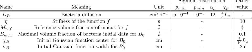
Sigmoid distribution Other
Name Meaning Unit pmax pmin αp χp value
DB Bacteria diffusion cm2d−1 5.10−4 10−5 12 45Lx
-η Stifness of the functionf s - 10
Mref Reference volume fraction of mucus forf ∅ - 45
Bmax Maximal volume fraction of bacteria initial data for B0 ∅ - 0.1
χB Initial Gaussian function center forB0 cm - 107Lx
σB Initial Gaussian function width forB0 cm - 25
Table 2. Biophysical constants of the extended model
We suppose that the volume fraction of bacteria is small compared to the amount of mucus or liquid, which leads us to assume the interface diffusion to be constant. We also suppose that the diffusion of bacteria grows with the amount of liquid. We setPDB= (DB,max, DB,min, αB, χB) and take
−2 −1 0 1 2 0
0.5 1
x
V
olume
fraction
(a)t= 0 day
−2 −1 0 1 2
0 0.5 1
x
(b)t= 12 days
−2 −1 0 1 2
0 0.5 1
x
(c)t= 50 days
Figure 10. Cut view of mucus (green continuous line) and bacteria (red dashed line) volume
fractions at different times aty=−Ly
2 for initial mucus profileM0,s.
For the sake of simplicity, we assume thatB0 depends only on the horizontal coordinate with a profile defined
by Gaussian functions centered on the interfaces liquid/mucus (see Fig. 10a)
B0(x, y) =Bmaxexp −
(x+χB)
2
2 (Lx/σB)
2
!
+Bmaxexp −
(x−χB)
2
2 (Lx/σB)
2
!
. (21)
The parameters are collected in Table 2. Eq. (18) is treated like the conservation equation forM. The Poisson equation (20) is discretized with the VF4 scheme on pressure cells. The mean value in the right hand side, as well as the constraint onR
φ dX, are approached by a suitable quadrature rule. We are led to solve an invertible linear system by introducing a Lagrange multiplier.
As in Section 5, we discuss the influence of the boundary data on Γin, depending whether or notuinvanishes,
and we check the behavior of the system when the mucus layer is perturbed. On Fig. 10b, the initial data for the mucus is a sigmoidal functionM0,s anduin= 0. We observe a neat concentration of the bacteria community
at the abscissa x = ±1.4 where the mucus volume fraction is close to Mref until t = 12 days. Then, the
amount of bacteria starts to decrease and after 50 days, see Fig. 10c the volume fraction of bacteria is almost zero: the model is not able to conserve a bacterial population in the gut. Surprisingly enough, the behavior is different when we keepuin= 0 and we change the initial data for the mucus toM0,g, see Fig. 11a. A steady
state, represented in Fig. 11b, is reached after 10 days: the profiles are indeed the same after 100 days, see Fig. 11c. In this state the bacterial community concentrates at the interface mucus/liquid, where the mucus volume fraction takes the value Mref = 0.4. The mucus profile is slightly sharper than initially.
It is interesting to study the influence of the horizontal velocity at Γin. Instead of imposinguin= 0 as above,
we now setuin6= 0 as given by the iteration procedure at Sec. 5.1. Mucus and bacteria profiles att= 50 and
t= 140 days are displayed on Fig. 12 for the sigmoidal initial dataM0,s. Changing the boundary condition for
uinhas completely changed the large time profiles: instead of a bacteria wash out, we observe an overgrowth of
−2 −1 0 1 2 0
0.5 1
x
V
olume
fraction
(a)t= 0 day
−2 −1 0 1 2
0 0.5 1
x
(b)t= 10 days
−2 −1 0 1 2
0 0.5 1
x
(c)t= 100 days
Figure 11. Cut view of mucus (green continuous line) and bacteria (red dashed line) volume
fractions at different times aty=−Ly
2 for initial mucus profileM0,g.
−2 −1 0 1 2
0 0.5 1
x
V
olume
fraction
(a)t= 0 day
−2 −1 0 1 2
0 0.5 1
x
(b)t= 50 days
−2 −1 0 1 2
0 0.5 1
x
(c)t= 140 days
Figure 12. Cut view of mucus (green continuous line) and bacteria (red dashed line) volume
fractions at different times at y = −Ly2 for M0,s and uin 6= 0 in the iterative procedure of
Sec. 5.1.
driven by chemotactic mechanisms, makes the model more sensitive, in particular with respect to uncertainties on the horizontal velocities, and its behavior is more intricate. This preliminary attempt provides interesting and relevant avenues for reflection, that will be further investigated elsewhere.
We finally investigate the recovery of the mucus layer when the initial condition is perturbed and the bacterial population is present. We take the same protocol as in Section 5. We start withM =M0,p att= 0 and take
the result of the iterative process as boundary condition on the boundary. The bacteria population initial distribution is sigmoidal until y = −4 and uniformly zero for −4 ≥ y ≥ −Ly. Several snapshots of the
t= 0 day t= 1 day t= 2 days t= 3 days t= 5 days t= 50 days
Figure 13. Evolution in time of the disrupted mucus layer together with the chemotactic bacterial population. We present the mucus (upper row) and bacteria (lower row) volume fraction maps at different times in order to illustrate the reconstitution of the steady-state mucus layer when a chemotactic bacterial population is present.
8.
Conclusion
We have proposed a model, inspired from mixture theory, which is able to describe the formation of a stable layer of mucus in the gut. The modelling relies on a short list of simple biological mechanisms — mucus production, liquid pumping, viscosity discrepancies between liquid and mucus, relevant inflow. Interaction with populations of bacteria can be incorporated in the equations, and the model reproduces the mucus layer flattening due to the penetration of the bacteria into the luminal part of the mucus layer. Such a model can take into account different biological knowledges to contribute to a better understanding of the microbial population dynamics and the host-microbiota interactions, especially through the mucus layer. This set of PDE can be used to investigate several pathological disorders of the mucus. For instance, by modifying the shape of the viscosity functionM 7→µ(M) we can describe rheological disorders due to mucin composition or conformation. Through the functionsfM andfL, we can account for mucus layer disruptions that arise in several bowel diseases, such
as the inflammatory bowel disease (IBD).
take into account the fluid/structure interactions that occur during peristaltism: the periodic contraction of the mucosa produces longitudinal traveling waves that ease the intestinal transit. Such a difficulty is common in the modeling of biological flows [1]. Accounting for the bacterial gas production is also an issue since it can influence the intestinal fluids flows. We are using a model based on mixture theory, which involves a closure relation describing diffusion effects. The definition of the diffusion coefficients is a crucial modeling issue. It enters both in the equation in the domain and in the boundary conditions for the constituents volume fractions. It would be natural to work with coefficients that depend on the mucus volume fraction, thus inducing further non linearities in the equations. Here, we have adopted a quite phenomelogical viewpoint by imposing a specific space-dependent profile to the coefficients DM, DL. The formula should be understood as a rough way to
describe the complex interaction of the mucus layer with the gut wall. The knowledge of these intercations is not well–advanced but it is clear from the observation that they are mechanisms able to keep the mucus attached to the wall. For instance, it would be interesting to take into account more precisely the impact of the microscopic nature of this interaction on the diffusion distribution through suitable homogeneization methods. The model for the bulk velocity could also incorporate additional viscosity term, as described in Remark 2.1, which would equally impact, and possibly improve, the definition of the boundary conditions. In order to describe more accurately the mucus stratification, the definition of the viscosity function should be improved, taking into account the different rheological properties of the mucus layers. Another relevant modeling option would be to set up a model with momentum balance equations for the velocities uM, uLof the constituents.
Finally, we have adopted a quite naive and phenomenological description of the chemotactic mechanisms that bacteria are subjected to; future developments should try to reflect more closely the biological mechanisms.
The work presented in this paper is the result of a fruitful collaboration that took place during the CEMRACS 2015. We warmly thank the organizers of the 2015 edition of the CEMRACS: Emmanuel Fr´enod (UBS Vannes), Emmanuel Maitre (U. Grenoble), Antoine Rousseau (Inria Montpellier), St´ephanie Salmon (URCA Reims), and Marcela Szopos (U. Strasbourg). We also thank the referees for useful remarks and comments regarding the manuscript.
References
[1] L. Baffico, C. Grandmont, and B. Maury. Multiscale modeling of the respiratory tract.Math. Models Meth. Appl. Sc., 20(1):59– 93, 2010.
[2] F. Boyer and P. Fabrie.Mathematical tools for the study of the incompressible Navier-Stokes equations and related models, volume 183 ofApp. Math. Sc.Springer Science & Business Media, 2012.
[3] C.-H. Bruneau and P. Fabrie. Effective downstream boundary conditions for incompressible Navier–Stokes equations.Int. J. Numer. Meth. in Fluids, 19(8):693–705, 1994.
[4] C.-H. Bruneau and P. Fabrie. New efficient boundary conditions for incompressible navier-stokes equations : a well-posedness result.ESAIM: M2AN, 30(7):815–840, 1996.
[5] R. Chatelin.Numerical methods for 3D Stokes flow: variable viscosity fluids in a complex moving geometry; application to biological fluids. Phd thesis, Universit´e Paul Sabatier - Toulouse III, November 2013.
[6] F. Clarelli, C. Di Russo, R. Natalini, and M. Ribot. A fluid dynamics model of the growth of phototrophic biofilms.J. Math. Biol., 66(7):1387–1408, 2013.
[7] B. J. Debusschere, H. N. Najm, P. P´ebay, O. M. Knio, R. G Ghanem, and O. P. Le Maˆıtre. Numerical challenges in the use of polynomial chaos representations for stochastic processes.SIAM J. Sc. Comput., 26(2):698–719, 2004.
[8] G. Evans.Practical numerical integration. Wiley New York, 1993.
[9] R. Eymard, T. Gallou¨et, and R. Herbin. Finite volume methods. InHandbook of numerical analysis, Vol. VII, Handb. Numer. Anal., VII, pages 713–1020. North-Holland, Amsterdam, 2000.
[10] T. Gerstner and M. Griebel. Numerical integration using sparse grids.Numer. Algo., 18(3-4):209–232, 1998.
[11] P. Gniewek and A. Kolinski. Coarse-Grained Modeling of Mucus Barrier Properties.Biophys. J., 102(2):195 – 200, 2012. [12] F. H. Harlow and J. E. Welch. Numerical calculation of time–dependent viscous incompressible flow of fluid with free surface.
Phys. Fluids, 8(12):2182–2189, 1965.
[13] M. E. V. Johansson, J. M. H. Larsson, and G. C. Hansson. The two mucus layers of colon are organized by the muc2 mucin, whereas the outer layer is a legislator of host–microbial interactions.Proc. Nat. Acad. Sc., 108(Supplement 1):4659–4665, 2011. [14] M. K. Kwan, W. M. Lai, and C. Van Mow. A finite deformation theory for cartilage and other soft hydrated connective
[15] Samuel K Lai, D Elizabeth O’Hanlon, Suzanne Harrold, Stan T Man, Ying-Ying Wang, Richard Cone, and Justin Hanes. Rapid transport of large polymeric nanoparticles in fresh undiluted human mucus.Proceedings of the National Academy of Sciences, 104(5):1482–1487, 2007.
[16] R. Mu˜noz Tamayo, B. Laroche, E. Walter, J. Dor´e, and M. Leclerc. Mathematical modelling of carbohydrate degradation by human colonic microbiota.J. Theoret. Biol., 266(1):189–201, September 2010.
[17] E. Novak and K. Ritter. High dimensional integration of smooth functions over cubes.Numer. Math., 75(1):79–97, 1996. [18] L. Preziosi and A. Tosin. Multiphase modelling of tumour growth and extracellular matrix interaction: mathematical tools
and applications.J. Math. Biol., 58(4-5):625–656, 2009.
[19] K. R. Rajagopal and L. Tao.Mechanics of mixtures. Series on Advances in Mathematics for Applied Sciences. World Scientific, Singapore, 1995.
[20] J.-C. Rambaud and J.-P. Buts.Gut microflora: digestive physiology and pathology. John Libbey Eurotext, 2006.
[21] J. L. Round and S. K. Mazmanian. The gut microbiota shapes intestinal immune responses during health and disease.Nat. Rev. Immunol., 9(5):313–323, May 2009.
[22] I. M. Sobol’. On sensitivity estimation for nonlinear mathematical models.Matematicheskoe Modelirovanie, 2(1):112–118, 1990.
[23] A. Swidsinski and V. Loening-Baucke.Functional Structure of Intestinal Microbiota in Health and Disease, pages 211–254. John Wiley & Sons, Inc., 2013.