N. Champagnat, T. Leli`evre, A. Nouy, Editors
HASTINGS-METROPOLIS ALGORITHM ON MARKOV CHAINS FOR
SMALL-PROBABILITY ESTIMATION
∗,∗∗Franc
¸ois Bachoc
1,2, Achref Bachouch
3and Lionel Lenˆ
otre
4,5Abstract. Shielding studies in neutron transport, with Monte Carlo codes, yield challenging problems of small-probability estimation. The particularity of these studies is that the small probability to estimate is formulated in terms of the distribution of a Markov chain, instead of that of a random vector in more classical cases. Thus, it is not straightforward to adapt classical statistical methods, for estimating small probabilities involving random vectors, to these neutron-transport problems. A recent interacting-particle method for small-probability estimation, relying on the Hastings-Metropolis algorithm, is presented. It is shown how to adapt the Hastings-Metropolis algorithm when dealing with Markov chains. A convergence result is also shown. Then, the practical implementation of the resulting method for small-probability estimation is treated in details, for a Monte Carlo shielding study. Finally, it is shown, for this study, that the proposed interacting-particle method considerably outperforms a simple Monte Carlo method, when the probability to estimate is small.
R´esum´e. Dans les ´etudes de protection en neutronique, celles fond´ees sur des codes Monte-Carlo posent d’importants probl`emes d’estimation de faibles probabilit´es. La particularit´e de ces ´etudes est que les faibles probabilit´es sont exprim´ees en termes de lois sur des chaines de Markov, contrairement `
a des lois sur des vecteurs al´eatoires dans les cas les plus classiques. Ainsi, les m´ethodes classiques d’estimation de faibles probabilit´es, portant sur des vecteurs al´eatoires, ne peuvent s’utiliser telles qu’elles, pour ces probl`emes neutroniques. Un m´ethode r´ecente d’estimation de faibles probabilit´es, par syst`eme de particules en int´eraction, reposant sur l’algorithme de Hastings-Metropolis, est pr´esent´ee. Il est alors montr´e comment adapter l’algorithme de Hastings-Metropolis au cas des chaines de Markov. Un r´esultat de convergence est ainsi prouv´e. Ensuite, il est expliqu´e en d´etail comment appliquer la m´ethode obtenue `a une ´etude de protection par Monte-Carlo. Finalement, pour cette ´etude, il est montr´e que la m´ethode par syst`eme de particules en int´eraction est consid´erablement plus efficace qu’une m´ethode par Monte Carlo classique, lorsque la probabilit´e `a estimer est faible.
∗The work presented in this manuscript was carried out in the framework of the REDVAR project of the CEMRACS 2013 ∗∗ This work was financed by the Commissariat `a l’´energie atomique et aux ´energies alternatives (CEA)
1 Department of Statistics and Operations Research, University of Vienna, Oskar-Morgenstern-Platz 1, A-1090 Vienna 2 When the work presented in this manuscript was carried out, the author was affiliated to CEA-Saclay, DEN, DM2S, STMF, LGLS, F-91191 Gif-Sur-Yvette, France and to the Laboratoire de Probabilit´es et Mod`eles Al´eatoires, Universit´e Paris VII 3 Institut f¨ur Mathematik, Humboldt-Universit¨at zu Berlin, Unter den Linden 6, D-10099, Berlin, Germany
4 Inria, Research Centre Rennes-Bretagne Atlantique, Campus de Beaulieu 35042 Rennes Cedex France 5 Universit´e de Rennes 1, Campus de Beaulieu 35042 Rennes Cedex France
c
EDP Sciences, SMAI 2015
1.
Introduction
The study of neutronics began in the 40s, when nuclear energy was on the verge of being used both for setting up nuclear devices like bombs and for civil purposes like the production of energy. Neutronics is the study of neutron population in fissile media that can be modeled using the linear Boltzmann equation, also known as the transport equation. More precisely, it can be subdivided in two different sub-domains. On the one hand, criticality studies aim at understanding the neutron population dynamics due to the branching process that mimics fission reaction (see for instance [23] for a recent survey on branching processes in neutronics). On the other hand, when neutrons are propagated through media where fission reactions do not occur, or can safely be neglected, their transport can be modeled by simple exponential flights [24]: indeed, between each collisions, neutrons travel along straight path distributed exponentially.
Among this last category, shielding studies allow to size shielding structures so as to protect humans from ionizing particles, and imply, by definition, the attenuation of initial neutron flux typically by several decades. For instance, the vessel structure of a nuclear reactor core attenuates the thermal neutron flux inside the core by a factor roughly equal to 1013. Many different national nuclear authorities require shielding studies of
nuclear systems before giving their agreement for the design of these systems. Examples are reactor cores, but also devices for nuclear medicine (proton-therapy, gamma-therapy, etc). The study of those nuclear systems is complicated by 3-dimensional effects due to the geometry and by non-trivial energetic spectrum that can hardly be modeled.
Since Monte Carlo transport codes (like MCNP [18], Geant4 [1], Tripoli-4 [9]) require very few hypotheses, they are often used for shielding studies. Nevertheless, those studies represent a long-standing numerical chal-lenge for Monte Carlo codes in the sense that they schematically require to evaluate the proportion of neutrons that “pass” through the shielding system. This proportion is, by construction, very small. Hence a shielding study by Monte Carlo code requires to evaluate a small probability, which is the motivation of the present paper.
There is a fair amount of literature on classical techniques for reducing the variance in these small-probability estimation problems for Monte Carlo codes. Those techniques often rely on a zero-variance scheme [2, 16, 17] adapted to the Boltzmann equation, allied with weight-watching techniques [3]. The particular forms that this scheme takes when concretely developed in various transport codes range from the use of weight windows [5, 16–18], like in MCNP, to the use of the exponential transform [4, 9] like in Tripoli-4. Nowadays, all those techniques have proven to be often limited in view of fullfilling the requirements made by national nuclear authorities for the precise measurements of radiation, which standards are progressively strengthened. Thus, new variance reduction techniques have been recently proposed in the literature (see for instance [10] for the use of neural networks for evaluating the importance function).
This paper deals with the application of the recent interacting-particle method developed in [12], which has interesting theoretical properties and is particularly efficient in various practical cases. Nevertheless, the application is not straightforward, since the method in [12] is designed for finite-dimensional problems, while the output of a neutron transport Monte Carlo code consists of a trajectory of the stochastic process driving the neutron behavior.
an algorithm for Bayesian estimation is proposed . However, the law to sample was simpler than the path distribution of a Markov chain and the state space totally different. Thus, our contribution is two-fold: first, we show how the Hastings-Metropolis algorithm can be extended to the case of Markov chains that are absorbed after finite time, and second we adapt the resulting interacting-particle method to the Monte Carlo simulation of a monokinetic particle in a simplified but realistic shielding system. We perform several numerical simulations which show that the smaller the probability to estimate is, the more the method we propose clearly outperforms a simple Monte Carlo method.
In what follows, we start with a short introduction to the interacting-particle method [12] and highlight the need of the Hastings-Metropolis algorithm (Section 2). Then, we dedicate a consequent work to prove the validity and the convergence of the Hastings-Metropolis algorithm applied to Markov Chains very similar to the one used in neutronic in order to convince the reader of the adaptation (Section 3). After that, we present the aforementioned monokinetic particle model and give the actual equations for the small probability estimation method 1 (Section 4). At last, we show the obtained numerical results for shielding studies and discuss them
(Section 5).
2.
The interacting-particle method for small probability estimation
Let (Ω,F, P) be probability space, (S,S, Q) a measured space, X a random variable from (Ω,F, P) to
(S,S, Q) that can be sampled and Φ :S→Ran objective function, so thatφ(X) has a continuous cumulative
distribution function. We aim at estimating the probabilitypof the event Φ(X)≥l, for a given levell∈R. In
order to evaluatep, we choose to use the interacting-particle method introduced in [12].
2.1.
Theoretical version of the interacting-particle method
Let assume that we are able to sampleX conditionally to the event Φ(X)≥x, for anyx∈R. In this case,
the interacting-particle method [12] for estimatingp, described in the following algorithm, yields a conceptually convenient estimator ˆpwith explicit finite-sample distribution. The algorithm is parameterized by the number of particlesN.
Algorithm 2.1.
• Generate an iid sample (X1, .., XN), from the distribution of X, and initialize m = 1, X11 = X1, ...,
XN1 =XN andL1= min(Φ(X1), ..,Φ(XN)).
• WhileLm≤l do – Fori= 1, ..., N
∗ Set Xim+1 =Xim if Φ(Xim)> Lm, and elseXim+1=X∗, whereX∗ follows the distribution
ofX conditionally toΦ(X)≥Lm, and is independent of any other random variables involved
in the algorithm. – Setm=m+ 1.
– SetLm= min(Φ(X1m), ..,Φ(XNm)).
• The estimate of the probability pispˆ= (1− 1 N)
m−1.
For eachN <∞, the estimator ˆphas an explicit distribution which is detailed in [12]. This reference exhibits two properties of ˆp: the estimator is unbiased and an asymptotic 95% confidence interval, forN large, has the following form
Ipˆ=
"
ˆ
pexp −1.96
r
−log ˆp N
!
,pˆexp 1.96
r
−log ˆp N
!#
. (1)
We note that the eventp∈Ipˆis asymptotically equivalent to the event ˆp∈Ip, withIp as in (1) with ˆpreplaced
byp. We mean that the probabilities of the two events converge to 0.95 and the probability of their symmetric difference converges to 0 asN → ∞. The asymptotic equivalence holds because log(ˆp) is asymptotically normal with mean log(p) and variance−log(p)/N [12]. We will use this property in Section 5.
2.2.
Practical implementation using the Hastings-Metropolis algorithm
In many practical cases, the previous algorithm is inapplicable, as it relies on the strong assumption of being able to exactly sample X conditionally to Φ(X)≥t, for anyt∈R. Subsequently, the authors of [12] propose to use the Hastings-Metropolis algorithm to simulate this conditional distribution. This method requires the following assumptions:
• The distribution ofX has a probability distribution function (pdf)f with respect to (S,S, Q). For any x∈S we can computef(x).
• We have a transition kernel on (S,S, Q) with conditional pdf κ(x, y) (pdf at y conditionally to x). [Throughout this paper,κis called the instrumental kernel.] We are able to sample fromκ(x, .) for any x∈S and we can computeκ(x, y) for anyx, y∈S.
Let t∈ Rand x∈S so that Φ(x) ≥t. Then, the following algorithm enables to, starting fromx, sample
approximately with the distribution of X, conditionally to Φ(X) ≥t. The algorithm is parameterized by a number of iterationsT ∈N∗.
Algorithm 2.2.
• Let X =x.
• Fori= 1, ..., T
– Independently from any other random variable, generateX∗ following theκ(X, .)distribution. – IfΦ(X∗)≥t
∗ Let r= ff((XX∗))κκ((X,XX∗,X∗)).
∗ With probability min(r,1), letX =X∗. • ReturnXT ,t(x) =X.
For consistency, we now give the actual interacting-particle method, involving Algorithm 2.2. This method is parameterized by the number of particlesN and the number of HM iterationsT.
Algorithm 2.3.
• Generate an iid sample (X1, .., XN) from the distribution of X and initialize m = 1, X11 = X1, ...,
X1
N =XN andL1= min(Φ(X1), ..,Φ(XN))and.
• WhileLm≤l do – Fori= 1, ..., N
∗ If Φ(Xm
i )> Lm, setXim+1=Xim.
∗ Else sample an integer J uniformly in the set {1≤j ≤N; Φ(Xm
j )> Lm}. Apply Algorithm
2.2 with number of iterations T, starting point Xm
J and with threshold value t=Lm. Write
XT ,Lm(X
m
J )for the output of this algorithm and letX m+1
i =XT ,Lm(X
m J ). – Setm=m+ 1.
– SetLm= min(Φ(X1m), ..,Φ(XNm)).
• The estimate of the probability pispˆ= (1− 1 N)
m−1.
The estimator ˆp of Algorithm 2.3 is the practical estimator that we will study in the numerical results of Section 5. In [12], it is shown that, when the spaceSis a subset ofRd, under mild assumptions, the distribution
of the estimator of Algorithm 2.3 converges, asT →+∞, to the distribution of the ideal estimator of Algorithm 2.1. For this reason, we call the estimator of Algorithm 2.1 the estimator corresponding to the case T = +∞. We also call the confidence intervals (1) the confidence intervals of the caseT = +∞.
3.
An extension of Hastings-Metropolis algorithm to path sampling
3.1.
Reformulation of the Markov chain describing the neutronic problem
In many neutronic models, the dynamics of the collisions are described by a Markov chain (Xn)n≥0 with
values in Rd and which possesses a probability transition functionqand an initial positionX0 =α. Since the
detection problem occurs only in a restricted area, we decide to change this description using a censorship. Such a trick will be of great help for the theoretical treatment developed later.
Let D be an open bounded subset of Rd with ∂D its boundary. Because D is the domain of interest, we
rewrite the transition function of the process (Xn)n≥0 as follows
k(x, dy) = (q(x, y)1D(y)dy+qx(DC)δ∆(dy))1D(x) +δ∆(dy)1∆(x)
where ∆ is a resting point and
qx(DC) =
Z
DC
q(x, y)dy.
This kernel describes the following dynamic:
• while (Xn)n≥0 is insideD, it moves according to the transition kernel q that reflects the dynamics of
the collision and can push the neutron outsideD .
• when (Xn)n≥0enters inDC, it is killed and sent to the resting point ∆ where it stays indefinitely. This
way we keep only the information occurring exactly insideD.
We call this stochastic process a boundary absorbed markov chains (BAMC).
3.2.
Reminder of the Hastings-Metropolis algorithm
The Hastings-Metropolis algorithm is a generic procedure used to sample a distribution γ that admits a density with respect to a measure Π [14, 20]. The idea of this algorithm is to define a Markov chain (Yn)n≥0
with a transition kernel Γ that converges to γin some sense that will be discussed later. In order to construct (Yn)n≥0, the Hastings-Metropolis procedure uses an instrumental Markov chain (Zn)n≥0 and an
acceptation-rejection functionr. We will denote byκthe probability transition kernel of (Zn)n≥0and call it the instrumental
kernel. The main hypothesis required on κand Γ for the algorithm is that they admit a density with respect to the measure Π. A Step by step description of the algorithm:
• Introduce a starting pointxand use it to sample a potential new positiony of (Zn)n≥0.
• Accepty and set x=y or reject it usingr. • return the position xas the sample.
The more this procedure is repeated the more approximation is reliable. We can write the transition kernel Γ of (Zn)n≥0 as follows
Γ(u, dv) =κ(u, v)dΠ(v) +r(u)δu(dv)
where
κ(u, v) =
(
κ(u, v)r(u, v), ifx6=y,
0, ifx=y,
and
r(u) = 1−
Z
κ(u, v)dΠ(v).
Π is invariant for Γ [22]. we refer to the literature for more details [14, 19, 20, 22]. We choose here:
r(u, v) =
min
γ(v)κ(v, u)
γ(u)κ(u, v),1
, ifγ(u)κ(u, v)>0
1, ifγ(u)κ(u, v) = 0
.
3.3.
Definition of a point absorbed Markov chain on a sphere
The extension of the Hastings-Metropolis algorithm to sample the paths of a BAMC is quite natural and has been already used in several numerical methods. But, as far as we know, there is still no rigorous proof for the convergence. We give a proof for the below defined point absorbed Markov chain (PAMC) on a sphere S that can be linked through topological results to the BAMC presented earlier .
LetB be a ball included in the unit ball ofRd such that 0∈∂B. We introduce the sphereS=∂B and the
notationS0=S− {0}. We denote byλthe Lebesgue measure restricted on S0. Let remark thatλis the same
on bothS0 andS, and that the densities are identical. As a result,λwill also stand for the Lebesgue measure
onS. We define a PAMC on S as the stochastic process (Mn)n≥0 with a probability transition function
m(x, dy) = (p(x, y)1S0(y)dy+Px(0)δ0(dy))1S0(x) +δ0(dy)10(x).
where
(1) pis a transition function onS having a density with respect toλ, (2) (Px(0))x∈S0 is a family of positive real numbers,
(3) For everyx∈S0,
Z
S
p(x, y)1S0(y)dy+Px(0)δ0(dy) = 1,
(4) mis such that (Mn)n≥0 is almost surely absorbed in finite time.
(5) For every (x, y)∈S2 0,
m < p(x, y)< M,
(6) For everyx∈S0,
Px(0)> c.
The proof of the convergence in total variation the Hastings-Metropolis algorithm extended to the above PAMC will be performed using results provided by some classical references [19, 21, 22]. These results suppose that the state space of the HM chain is a metric, locally compact and separable topological space. In order to check these properties, we now consider a few topological questions.
We start by pointing out that the state space of a PAMC on S is the space of sequences with values inS and equal to zero after some finite time:
c0(S) ={(un)n≥0∈SN:∃n0∈N,∀n≥n0, un = 0},
We equipped this space with the norm:
kuk∞= max
n≥0kunkR
d.
This state space have the properties mentioned earlier if we accept the following:
Claim 3.1. There exists a locally compact and separable topology on the space c0(S) that can be equipped
with a metric. In addition, the Borel σ-algebra generated by this topology coincides with B(c0(S)) the one
generated byk · k∞.
Remark 3.2. There is a classical result that allows to expect that this result is true: the continuous injection of c0(S)) into l∞(Rd) or into l2(Rd). In fact, l∞(Rd) can be equipped with the weak-star topology which is
locally compact andl2(
A PAMC onS is a random variable:
M : (Ω,F,P) 7→ (c0,B(c0(S)))
ω 7→ (Mn(ω))n≥0,
if we use theσ-algebra:
F =
+∞
O
i=0
B(S),
generated by the Borelian cylinders of finite dimension. Therefore, the following result shows the measurability of the process (Mn)n≥0 with respect to the Borelσ-algebra generated byk · k∞.
Proposition 3.3. The traceσ-algebraF|c0(S) on the subspacec0(S)of F is equal toB(c0(S)).
Proof. Letpnbe the projection fromc0(S) inS which associatesuntou. This application is Lipschitz. In fact,
letuand v be in c0(S), we havekun−vnkRd ≤ ku−vk∞. Consequently, every projection is measurable and we have the following inclusion:
F|c0(S)⊂ B(c0(S)).
We know thatB(c0(S)) is generated by the balls of radiusρ∈Qand center pointsu∈T whereT is a dense
subset of S, since c0(S) equipped with the norm k · k∞ is separable. Thus, it is enough to show that the ball B(ρ, u) is inF|c0(S). In order to prove that, we write:
B(ρ, u) =
+∞
\
n=0
{v∈c0(S),kun−vnkRd≤ρ}.
Since each member of this intersection is inFc0, we have the opposite inclusion:
B(c0(S))⊂ Fc0(S).
Remark 3.4. This proof can be considered as an adaption of a classical result for the Brownian Motion [7].
3.4.
Density of a point absorbed Markov chain on a sphere
In order to prove the converge of the HM algorithm, we must show that the law of a PAMC on the sphereS admits a density with respect to a measure onc0(S). Since we deal with a Markov process, we do not have to
take the initial law into account. As a result, we just have to find a density for the law of the process conditioned to start from a.
Without loss of generality, we can shift the element of c0(S) and rewrite them (un)n≥1. Let introduce a
partition of the spacec0(S) using the subsets (An)n≥0 consisting of:
A0={u∈c0(S) :uk = 0,∀k≥1},
An={u∈c0(S) :uk ∈S0,∀k≤nanduk= 0,∀k > n},∀n≥1
and the family of applications (πn)n≥0defined as:
πn:c0(S)7→Sn
(un)n≥17→(u1,· · · , un).
We define the measure Π onc0(S) as follows:
and, for eachn≥1,
Π|An(du) =λ
n(π n(du)),
whereλn is the Lebesgue measure on Sn. We have the following result:
Proposition 3.5. The law of a point absorbed Markov chain (Mn)n≥0 on the sphere S, conditioned to start
froma is absolutely continuous with respect toΠ.
Proof. Let γ be the distribution of (Mn)n≥0 conditioned to start from a. We fix A ∈ B(c0(S)) such that
Π(A) = 0. Since A0 is an atom for Π, Π(A) = 0 implies that A0∩A=∅. Thus, we just have to check that
γ(A∩An) = 0, for everyn≥1, and to apply the fact that
γ(A) =
+∞
X
n=0
γ(A∩An) = 0.
Subsequently, using the Markov property, we write:
γ(A∩An) =Pa((M1,· · ·, Mn)∈πn(A∩An), Mn+1= 0)
=Pa((M1,· · ·, Mn)∈πn(A∩An))PMn(0)
≤
Z
πn(A∩An)
p(a, u1)· · ·p(un−1, un)du1· · ·dun
sincePx(0)≤1, for everyx∈S0. The desired result follows when we recall thatpis absolutely continuous with
respect to λandλ(πn−1(A∩An)) = 0.
This last result allows us to use the Radon-Nykodym-Lebesgue theorem that provide the existence of a density with respect to Π for the distributionγ. The point is now to exhibit this density.
Proposition 3.6. The density with respect to Π of the law of the PAMC on the sphere (Mn)n≥0 conditioned
to start from the pointa6= 0, is
Pa(0)1A0(u) +
+∞
X
n=1
p(a, u1)· · ·p(un−1, un) 1S−{0}(u1)· · ·1S−{0}(un)Pun(0) 1An(u).
In addition, this density is normalized.
Proof. In order to prove this result, we must show, for each Borelian cylinder of finite dimensionC∈ F, that
γ(C) =
Z
C
Pa(0)1A0(u) +
+∞
X
n=1
p(a, u1)· · ·p(un−1, un) 1S−{0}(u1)· · ·1S−{0}(un)Pun(0)dΠ(du).
We start by recalling that a Borelian cylinder of finite dimension has the formC0× · · · ×Cm×S× · · · and the
fact that
γ(C) =
+∞
X
n=0
since the sequence (An)n≥0 forms a partition ofC0(S). Ifn >0, we can observe that, forn < m,
γ(C∩An) =Pa(M1∈C1− {0},· · · , Mn∈Cn− {0}, Mn+1= 0)
=
Z
C1−{0}
· · ·
Z
Cn−{0}
p(a, u1)· · ·p(un−1, un)Pun(0)du1· · ·dun
=
Z
πn(C∩An)
p(a, u1)· · ·p(un−1, un)Pun(0)du1· · ·dun
=
Z
C
p(a, u1)· · ·p(un−1, un)Pun(0) 1An(u)dΠ(du)
or, forn > m,
γ(C∩An) =Pa(M1∈C1− {0},· · ·, Mm∈Cm− {0},· · · , Mn∈S− {0}, Mn+1= 0)
=
Z
C1−{0}
· · ·
Z
Cm−{0}
Z
S−{0} · · ·
Z
S−{0}
p(a, u1)· · ·p(xn−1, un)Pun(0)du1· · ·dun
=
Z
πn(C∩An)
p(a, u1)· · ·p(un−1, un)Pun(0)du1· · ·dun
=
Z
C
p(a, u1)· · ·p(un−1, un)Pun(0) 1An(u)dΠ(du)
which show the first part of the result, since
γ(C∩A0) =Pa(M1= 0) =Pa(0) =
Z
C
Pa(0)δA0 =
Z
C
Pa(0)1A0(u)dΠ(du).
As it is not obvious in the proof, we show that the density is normalized using the fact that
P(T =n+ 1) =Pa(M1∈S− {0},· · ·, Mn∈S− {0}, Mn+1= 0)
=
Z
SN
p(a, u1)· · ·p(un−1, un)Pun(0)1An(u)dΠ(du),
and
P(T = 1) =Pa(M1= 0) =
Z
C
Pa(0)1A0(u)dΠ(du),
where T is the first time M reaches the absorbing point 0. In fact, this is enough when we know that T is
almost surely finished and thatP(T = 0) = 0.
3.5.
A Class of
Π
-irreducible instrumental kernels
The Hastings-Metropolis algorithm was originally designed for real random variables and has been widely used in this case. As a result, extensive studies have been been made to compare different instrumental kernels and show that they play a major role on the reliability of the samples. Since it is quite new to extend the algorithm to the PAMC on the sphereS, we only give here a simple admissible class of kernels.
The main property required by the Hastings-Metropolis algorithm on an instrumental kernel is the γ-irreducibility in the sense defined below, as it is a necessary condition for the convergence of the algorithm [19,22]. Subsequently, we introduce the following probability transition kernel onc0(S)× B(c0(S)) in term of its density
with respect to Π :
κ(u, dv) = Θ0(u)1A0(v) +
+∞
X
k=1
Θk(u)νk(u, v)1Ak(v)
(1) For eachu∈c0, the sum of the (Θk(u))k≥0is 1.
(2) For eachu∈c0 andk≥0, Θk(u)>0.
(3) For eachk≥1,νk(u, dv) is a probability transition kernel onSk0 having a density with respect toλk.
This statement ensures that κis a probability transition kernel onc0. We describe the behavior of the chain:
(1) We change the number of non-null points using the family (Θk(u))k≥0. For example, suppose that
u∈Am, thenumoves intoAk with the probability Θk(u). As a result, the chainuloses or gains points
different from 0. In the case consisting of adding new points, we choose to initialize all of them at a positionb∈S− {0}. Otherwise, by losing, we mean that the last m−kpositions are set to 0.
(2) We use a classical instrumental kernel on the finite dimensional vector of non-null positions.
Before proving any property on this kernel, we give a set of definitions to understand the concept of the irreducibility of a Markov chain:
Definition 3.7. LetGbe a topological space,Gaσ-algebra onG,ma probability measure andµa probability transition kernel. We say thatA∈ Gis attainable fromx∈Gif:
it exists n >1 such thatµn(u, A)>0,
and attainable fromx∈Gin one step ifµ(u, A)>0.
Definition 3.8. LetGbe a topological space,Gaσ-algebra onG,ma probability measure andµa probability transition kernel.
(1) B∈ G ism-communicating if
∀x∈B,∀A∈ G such thatA⊂B,m(A)>0, Ais attainable fromx.
(2) B∈ G is quicklym-communicating if
∀x∈B,∀A∈ Gsuch that A⊂B,m(A)>0, Ais attainable in one step fromx.
Definition 3.9. LetGbe a topological space,Gaσ-algebra onG,ma probability measure andµthe probability transition kernel of a Markov chain (Xn)n≥0.
(1) Gism-communicating, (Xn)n≥0 andµare saidm-irreducible.
(2) Gis quicklym-communicating, (Xn)n≥0andµare said stronglym-irreducible.
From [22], we know that: if κis Π-irreducible, thenκis also γ-irreducible since γ is absolutely continuous with respect to the measure Π. As a result, the result that follows provides the property required for the convergence which is aforementioned.
Proposition 3.10. If κis such that, for each k ≥1,νk(u, dv) is strongly λk-irreducible. Then,κ is strongly
Π-irreducible.
Proof. Let A ∈ B(c0) be a Π-positive subset and u ∈ c0 a sequence. In order to prove that κ is strongly
Π-irreducibility, we have to show thatκ(u, A)>0. Note that this result holds if, for eachk≥0,
A⊂Ak is Π-positive =⇒ A is attainable fromu∈c0.
Let fixk≥0 and assume thatA⊂Ak. From the definition ofκ, we have
κ(u, A) =
Z
A
Since Θk(u)>0 for everyk >0 andu∈c0(S), we only have to prove that
Z
A
νk(u, v)dv >0.
The absolute continuity and the fact thatνk(u, v) is stronglyλk-irreducible induce that
ifAis aλk-positive set, thenνk(u, A)>0.
and the result holds. Indeed, if we suppose the opposite, then we have a conflict with the strongλk-irreducibility,
since
ifA⊂Ak is a Π-positive set, thenA is aλk-positive set.
3.6.
Convergence of the extended Hastings-Metropolis algorithm
Before the proof of convergence of the algorithm, we give an example of (Θk(u))k≥0 and (νk(u, v))k≥1 such
thatκisγ-irreducible. LetGbe a random variable following the shifted geometric distribution onNandgthe
density of the uniform distribution onS0. For eachu∈c0(S), we set Θk(u) =P(G=k) and
νk(u, v) = k
Y
i=1
g(v).
The following theorem is the main theoretical result of this paper. It relies on the topological claim which provides the hypothesis required in the theoretical results used for the proof. We decide to present a theorem with relatively strong hypothesis in order to convince the reader of the convergence of the more complex case used in the numerical experiments.
Theorem 3.11. Let (Mn)n≥0 be a Point Absorbed Markov chain on S starting from a. We consider the
following instrumental kernel:
κ(u, dv) = Θ0(u)1A0(v) +
+∞
X
k=1
Θk(u)νk(u, v)1Ak(v)
satisfying the following hypothesis:
(1) For each u∈c0 andk≥0,
Θk(u) =P(G=k) where:
(a) Ga probability law onN.
(b) for everyk∈N,P(G=k)>0.
(2) for each k≥1,
νk(u, v) =h(u1, v1)· · ·h(uk, vk)
where:
(a) his a probability transition kernel onS0.
(b) his absolutely continuous with respect toλ. (c) his stronglyλ-irreducible.
(d) his symmetric: h(x, y) =h(y, x), for every(u, v)in S02.
Proof. The probability transition kernelhonS is stronglyg-irreducible, since it is absolutely continuous with respect toλand stronglyλ-irreducible. In addition, νk(u, v) is strongly λk-irreducible as a product of strongly
λ-irreducible kernel . Using Proposition 3.10, we conclude that the kernelκis stronglyγ-irreducible.
In order to prove the convergence the Hastings-Metropolis kernel Γ, we follow [22] which shows that we just have to show that Γ isγ-irreducible andγ{r(u)>0}>0 to obtain the convergence with respect to the topology of the total variation norm. Before starting the proof, we recall that
Γ(u, dv) =κ(u, v)Π(dv) +r(u)δu(dv)
where
κ(u, v) =
(
κ(u, v)r(u, v), ifu6=v,
0, ifu=v,
r(u) = 1−
Z
κ(u, v)Π(dv).
and
r(u, v) =
min
γ(v)κ(v, u)
γ(u)κ(u, v),1
, ifγ(u)κ(u, v)>0
1, ifγ(u)κ(u, v) = 0
.
We start by showing that Γ is stronglyγ-irreducible. LetA∈ B(c0) be aγ-positive subset andua sequence
ofc0(S) such thatu∈Al. We can establish that Γ is stronglyγ-irreductible if we prove that Γn(u, A)>0. We
use the approach developed in the proof of Proposition 3.10. Let fixk≥0 and suppose thatA⊂Ak. With the
second term in the expression of Γ and the fact that
r(u, v)≥ γ(v)κ(v, u) γ(u)κ(u, v),
it is enough to show that
κ(u, A) =
Z
A
κ(u, v)γ(v)κ(v, u) γ(u)κ(u, v)Π(dv)
=
Z
A
γ(v)κ(v, u)
γ(u) λ
k(dv)>0.
Moreover, we can suppose thatuis such thatγ(u)>0 onB ⊂A, else the result is proved since
κ(u, A) =
Z
A
κ(u, v)Π(dv)
andκis stronglyγ-irreducible. As result, we have
Z
A
γ(v)κ(v, u)
γ(u) λ
k(dv)≥ 1
γ(u)
Z
B
γ(v)κ(v, u)λk(dv).
Thereupon, we can suppose that it existsB0 ⊂B such thatγ(v)> C1, for eachv∈B0, sinceγ(A)>0. Thus,
we get that
Z
A
γ(v)κ(v, u)
γ(u) λ
k(dv)≥ C1
γ(u)
Z
B0
Using the symmetry ofh, we can rewrite:
Z
A
γ(v)κ(v, u)
γ(u) λ
k(dv)≥ C1
γ(u)
Z
B0
Θl(v)h(u1, v1)· · ·h(un, vn)dv1· · ·dvn ≥
C
γ(u) v∈infc0(S)
Θl(v),
and the strongγ-irreducibiblity follows from the hypothesis.
The last step consist of showing thatγ{r(u)>0}>0. From the definition of a PAMC, for everyl≥0, we know that γ(Al)>0. Supposev∈Ak withk < l. Then, for everyu∈Al, we have:
γ(v)κ(v, u) γ(u)κ(u, v) =
p(a, v1)· · ·p(vk−1, vk)Pvk(0) p(a, u1)· · ·p(ul−1, ul)Pul(0)
× Θl(v)
Θk(u)
× h(v1, u1)· · ·h(vl, ul)
h(u1, v1)· · ·h(uk, vk)
.
Sincehis symmetric, we can rewrite:
γ(v)κ(v, u) γ(u)κ(u, v) =
p(a, v1)· · ·p(vk−1, vk)Pvk(0) p(a, u1)· · ·p(ul−1, ul)Pul(0)
× Θl(v)
Θk(u)
×h(vk+1, uk+1)· · ·h(vl, ul).
Moreover,h(v,·) being absolutely continuous with respect to the Lebesgue measure on S,h(v, .) is continuous and bounded onS. But,his symmetric. Thus,his uniformly bounded onS and
γ(v)κ(v, u) γ(u)κ(u, v) ≤C2
p(a, v1)· · ·p(vk−1, vk)Pvk(0) p(a, u1)· · ·p(ul−1, ul)Pul(0)
× Θl(v)
Θk(u)
.
From the hypothesis on the transition kernel of a PAMC, we have:
γ(v)κ(v, u) γ(u)κ(u, v) ≤
C2
c ×
Mk
ml ×
Θl(v)
Θk(u)
.
Since the sum of the Θl(v) is finite for everyv ∈c0(S) and the same, the sequence (Θl(v))l≥0 converges to 0.
As a result, we can choosel such that
Θl(v)<
C
2
c ×
Mk
ml ×
1 Θk(u)
−1
.
Thus, for every u∈Alandv∈Ak,
γ(v)κ(v, u) γ(u)κ(u, v) <1, and, for everyu∈Al,
Z
κ(u, v) Π(dv)≤
Z
c0(s)−{Ak}
κ(u, v) Π(dv) +
Z
Ak
κ(u, v)γ(v)κ(v, u)
γ(u)κ(u, v)Π(dv)<1
which provides the desired results.
4.
Practical implementation for the monokinetic particle simulation
it is killed when it leaves the domain and also possibly in the domain. Thus, the notion of pdf for the space of monokinetic particle trajectories must be first defined, in a different way than in Section 3. Then, we present one and two-dimensional versions of the monokinetic particle model, the instrumental kernels we consider, and we give the corresponding explicit expressions of the unconditional and conditional pdf of the trajectories. The final version of Algorithm 2.3 for the monokinetic particle simulation is then summed up.
4.1.
General vocabulary and notation
Throughout Section 4, we consider a monokinetic particle (a particle with constant speed and yielding no subparticle birth) evolving in Rd, withd= 1,2. The birth of the particle takes place ats, which we write as
X0=s. Then, the trajectory of the monokinetic particle is characterized by its collision points, which constitute
a homogeneous Markov chain (Xn)n∈N∗ onR
d∪ {∆}with transition kernel
k(xn, dxn+1) =δ∆(dxn+1)1{xn = ∆}+{P(xn)δ∆(dxn+1) + [1−P(xn)]q(xn, xn+1)dxn+1}1{xn 6= ∆}. (2)
In the above display, P(xn) ∈ [0,1] is the probability of absorption for a collision taking place at xn ∈ Rd.
Absorption at collision nis here conventionally defined as Xn+1 = ∆ = 0∈Rd+1, which impliesXm = ∆ for
any m > n. We call ∆ the absorbed state, or resting point as in Section 3 and use the convenient convention that an absorbed monokinetic particle makes an infinite number of collisions at ∆. Finally, conditionally to the collision xn, the particle is scattered with probability 1−P(xn), in which case the next collision point has pdf
q(xn, .).
We assume here, similarly to Section 3, that the Markov chain (Xn)n∈N∗ has the property that absorption happens almost surely after a finite number of collisions. That is, almost surely, there exists m ∈ Nso that
Xn = ∆ for n ≥m. This assumption holds for example when P(xn) = 1 out of a compact set C ofRd and
where there exists a positive constant c so that q(x,Rd\C)≥cfor all x∈Rd, which is the case in Section 4.
We say that the monokinetic particle is active at time n, or atXn, or before collisionn, ifXn6= ∆.
Finally, note that the Markov Chain of the collision points (Xn)n∈N∗does not include the birth pointX0=s,
which entails no loss of information sincesis deterministic.
4.2.
The measured space of monokinetic particle trajectories
For further reference throughout Section 4, we define here the measured space (c0,S,Π) of the monokinetic
particle paths. We start by defining c0 andS.
Definition 4.1. Define
c0={(xn)n≥1∈ Rd∪ {∆}N
∗
:∃n0∈N∗,∀n < n0, xn6= ∆;∀n≥n0, xn= ∆}.
Let S be the smallest sigma-algebra on c0 containing the sets {x ∈ c0|x1 ∈ B1, ..., xn ∈ Bn, xn+1 = ∆}, for
n∈NandBi∈ B Rd, whereB Rdis the Borel sigma-algebra onRd.
We define forn≥0
An={x∈c0;∀1≤j ≤n:xj 6= ∆,∀k≥n+ 1 :xk= ∆}, (3)
that is the set of trajectories that are absorbed at collision pointn(so that they are in the absorbed state from collision pointn+ 1 and onward). Note that theAn, forn≥0, constitute a partition of c0. The existence of
the measure Π is now shown in the following proposition, which can be proved in the same way as in Section 3.
Proposition 4.2. There exists a unique measure Π on (c0,S) that verifies the following relation, for any
En={x∈An;x1∈B1, ..., xn ∈Bn}, withB1, ..., Bn∈ B Rdandn∈N:
Π(En) =λ(B1)...λ(Bn), (4)
4.3.
Description of the one-dimensional case and expression of the probability density
functions
4.3.1. A one-dimensional random walk
We consider that the monokinetic particle evolves in R. With the notation of (2), we set q(xn, .) as the
Gaussian pdf with mean 0 and varianceσ2and we setP(t) =1{t6∈(A, B)}+P1{t∈(A, B)}, withA <0< B
and 0< P <1. Thus, the particle travels with normally distributed increments, has a probability of absorption P at each collision point in the domain of interest (A, B) and is absorbed if it leaves this domain.
The following algorithm, when tuned with source points= 0, sums up how one can sample one-dimensional trajectories.
Algorithm 4.3. Objective: from a source point s ∈R and the parameters D= (A, B), σ2 andP, sample a trajectoryxas described above.
• Set i= 0,xi=sand “state = active”.
• While “state = active” do
– Samplexi+1 from theN(xi, σ2)distribution. – Ifxi+16∈ D
∗ Set “state = inactive”. – Ifxi+1∈ D
∗ With probability P, set “state = inactive”. – Seti=i+ 1.
• Return the infinite sequence(x1, ..., xi,∆, ...).
The event of interest is here that the monokinetic particle reaches the domain (−∞, A]. When using the interacting-particle method of Section 2, this event is expressed by Φ(x)≥0, with Φ(x) =A−infi∈N∗;xi6=∆xi. Note that, almost-surely, the infimum is taken over a finite number of points.
Although the two-dimensional case of Section 4.4 is more realistic, we address here absorption with positive probability at each collision point, which is an important features of shielding studies by Monte Carlo code. Furthermore, by setting P sufficiently large, and A sufficiently away from 0, we will see that we can tackle problems of estimation of arbitrary small probabilities. In Section 5, we will consider a probability small enough so that the interacting-particle method of Section 2 outperforms a simple Monte Carlo method.
4.3.2. Expression of the probability density function of a trajectory
We now give the expression of the pdf (with respect to the setting of Definition 4.1 and Proposition 4.2) of a trajectory obtained from the one-dimensional model above. We let (xi)i∈N∗ be the sequence of collision points (the trajectory) of a monokinetic particle. We letD= (A, B). We denoteφ(m, σ2, t) the pdf attof the
one-dimensional Gaussian distribution with meanm and varianceσ2.
Proposition 4.4. The pdf, with respect to (c0,S,Π) of Definition 4.1 and Proposition 4.2, of a trajectory
(xn)n∈N∗, sampled from Algorithm 4.3, is f(x) =P
n∈N∗1An(x)fn(x), with fn(x) =
n−1
Y
i=1
φ(xi−1, σ2, xi)(1−P)1{xi∈ D}
!
φ(xn−1, σ2, xn) (1{xn 6∈ D}+P1{xn∈ D}),
wherex0= 0by convention.
of randomness (the exact collision point at which the monokinetic particle leaves D) that does not impact the event of interest. This is nevertheless inevitable if one requires explicit evaluation of the pdf. Indeed, modifying the definition of trajectories and of pdf so that collision points out of the domain are not stored would add to the pdf expression the probability that, starting from a birth or scattering point in the domain D, the next collision point lies outsideD. This probability has an explicit expression in this one-dimensional case, but not in the framework of Section 4.4, and a fortiori not in shielding studies involving more complex Monte Carlo codes. Thus, to avoid evaluating this probability numerically each time a pdf of a trajectory is computed, we store the collision points outside the domainD.
The evaluation of a pdf like that of Proposition 4.4 is an intrusive operation on a Monte Carlo code. Indeed, it necessitates to know all the random-quantity sampling that are done when this code samples a monokinetic-particle trajectory. Thus, the Monte Carlo code is not used as a black box. Nevertheless, the computational cost of the pdf evaluation is of the same order as the computational cost of a trajectory sampling, and the same kind of operations are involved. Namely, both tasks require a loop which length is the number of collisions made by the monokinetic-particle before its absorption. Furthermore, for each random quantity that is sampled for a trajectory sampling, the pdf evaluation requires to compute the corresponding pdf. For example, in the case of Proposition 4.4, when a trajectory sampling requires to samplenGaussian variables andn orn−1 Bernoulli variables, the trajectory-pdf evaluation requires to compute the corresponding Gaussian pdf and Bernoulli probabilities.
Finally, the discussion above holds similarly for the two-dimensional case of Section 4.4.
4.3.3. Description of the trajectory perturbation method whenP = 0
For clarity of exposition, we present first the perturbation method whenP= 0. In this case, the monokinetic particle is a random walk onR, that is absorbed once it goes outsideD.
The perturbation method is parameterized by ˜σ2 > 0. Let us consider a historical trajectory (x i)i∈N∗,
absorbed at collisionn. Then, the set of birth and collision points of the perturbed monokinetic-particle is an inhomogeneous Markov chain (Yi)i∈N so that Y0 = 0. Ifi≤n−1, and if the perturbed monokinetic particle
is still in D at collision pointi, we have Yi+1 =Yi+i+1, where the (i)1≤i≤n are independent and where i
follows aN(xi−xi−1,σ˜2) distribution.
Similarly to the initial sampling, the perturbed monokinetic particle is absorbed at the first collision point outside D. If the collision point Yn of the perturbed monokinetic particle is in D (contrary to xn for the
initial trajectory), the sequel of the trajectory of the perturbed monokinetic particle is sampled as the initial monokinetic particle would be sampled if its collision pointnwasYn.
This conditional sampling method for perturbed trajectories is intrusive: it necessitates to change the sto-chastic dynamic of the monokinetic particle. Nevertheless, the new dynamic is here chosen as to have the same cost as the unconditional sampling, and to require the same type of computations. This is similar to the discussion following Proposition 4.4.
4.3.4. Expression of the probability density function of a perturbed trajectory whenP = 0
Proposition 4.5. Let us consider a historical trajectory (xi)i∈N∗, absorbed at collision n. The conditional pdf, with respect to (c0,S,Π) of Definition 4.1 and Proposition 4.2, of a trajectory (yn)n∈N∗ sampled from the procedure of Section 4.3.3, is κ(x, y) =P
m∈N∗1Am(y)fn,m(x, y)where, ifm≤n
fn,m(x, y) = m−1
Y
i=1
and if m > n,
fn,m(x, y) = n
Y
i=1
φ(yi−1+ (xi−xi−1),˜σ2, yi)1{yi∈ D}
×
m−1
Y
i=n+1
φ(yi−1, σ2, yi)1{yi∈ D}
φ(ym−1, σ2, ym)1{ym6∈ D},
wherex0=y0= 0by convention.
Similarly to the discussion following 4.4, the computation of the conditional pdf of a perturbed trajectory has the same computational cost as the sampling of this perturbed trajectory.
4.3.5. Description of the trajectory perturbation method whenP >0
In the general case whereP >0, the perturbation method is parameterized by ˜σ2>0 and 0< Q <1. Let us
consider a historical trajectory (xi)i∈N∗, absorbed at collisionn. As when P = 0, the set of birth and collision points of the perturbed monokinetic particle is an inhomogeneous Markov chain (Yi)i∈N, so that Y0 = 0. As
whenP= 0, we modify the increments of the initial trajectory, and, if the perturbed trajectory outsurvives the initial one, we generate the sequel with the initial distribution. Specifically to this case P >0, we perturb the absorption/non-absorption sampling by changing the initial values with probabilityQ.
More precisely, fori≤n−1 and if the perturbed monokinetic particle has not been absorbed before collision pointi, it is absorbed with probabilitymax(Q,1{Yi6∈D}). If it is scattered instead, we haveYi+1=Yi+i+1,
where the (i)1≤i≤n are independent and where i follows a N(xi−xi−1,˜σ2) distribution. If the perturbed
monokinetic particle has not been absorbed before collision point n, then it is absorbed ifYn6∈ D. IfYn∈ D,
the perturbed monokinetic particle is absorbed with probability (1−Q)1{xn∈ D}+P1{xn6∈ D}. As when
P = 0, if the perturbed monokinetic particle has not been absorbed before collision point Yn, the sequel of
the trajectory of the perturbed monokinetic particle is sampled as the initial particle would be sampled if its collision point nwasYn.
The idea is that, by selecting the difference betweenQand min(P,1−P), the closeness between the perturbed and initial trajectories can be specified, from the point of view of the absorption/non-absorption events. Finally, the following algorithm sums up how perturbed trajectories can be sampled.
Algorithm 4.6. Objective: from an initial trajectory xabsorbed at collision n and from the parametersD= (A, B),σ2,P,σ˜2 andQ, sample a perturbed trajectoryy as described above.
• Set i= 0,yi= 0and “state = active”.
• While “state = active” and i+ 1< ndo
– Sampleyi+1 from the N(yi+xi+1−xi,σ˜2)distribution. – Ifyi+16∈ D
∗ Set “state = inactive”. – Ifyi+1∈ D
∗ With probability Q, set “state = inactive”. – Seti=i+ 1.
• If “state = inactive”, stop the algorithm and return the infinite sequence (y1, ..., yi,∆, ...).
• If “state = active” do
– Sampleyi+1 from the N(yi+xi+1−xi,σ˜2)distribution. – Ifyi+16∈ D
∗ With probability (1−Q)1{xi+1∈ D}+P1{xi+16∈ D}, set “state = inactive”.
– Seti=i+ 1.
• If “state = inactive”, stop the algorithm and return the infinite sequence (y1, ..., yi,∆, ...).
• If “state = active” do,
– Apply Algorithm 4.3, withs=yi and write(˜x1, ...,x˜q,∆, ...)for the resulting trajectory. – Return the infinite sequence(y1, ..., yi,x˜1, ...,x˜q,∆, ...).
4.3.6. Expression of the probability density function of a perturbed trajectory whenP >0
Proposition 4.7. Let us consider a historical trajectory(xi)i∈N∗, absorbed at collision n. Lety0 =x0 = 0by
convention. The conditional pdf, with respect to(c0,S,Π)of Definition 4.1 and Proposition 4.2, of a trajectory
(yn)n∈N∗ sampled from Algorithm 4.6, isκ(x, y) =
P
m∈N∗1Am(y)fn,m(x, y)where, if m≤n−1, fn,m(x, y) =
m−1
Y
i=1
φ(yi−1+ (xi−xi−1),˜σ2, yi)(1−Q)1{yi∈ D}
φ(ym−1+ (xm−xm−1),σ˜2, ym) (Q1{ym∈ D}+1{ym6∈ D}),
if m=n,
fn,m(x, y) = n−1
Y
i=1
φ(yi−1+ (xi−xi−1),σ˜2, yi)(1−Q)1{yi∈ D}
φ(yn−1+ (xn−xn−1),σ˜2, yn)
(1{yn6∈ D}+ (1−Q)1{yn ∈ D}1{xn∈ D}+P1{yn∈ D}1{xn 6∈ D}),
and if m≥n+ 1,
fn,m(x, y) = n−1
Y
i=1
φ(yi−1+ (xi−xi−1),σ˜2, yi)(1−Q)1{yi∈ D}
φ(yn−1+ (xn−xn−1),σ˜2, yn)1{yn ∈ D}(Q1{xn∈ D}+ (1−P)1{xn6∈ D})
m−1
Y
i=n+1
φ(yi−1, σ2, yi)(1−P)1{yi ∈ D}
φ(ym−1, σ2, ym) (1{ym6∈ D}+P1{ym∈ D}).
4.4.
Description of the two-dimensional case and expression of the probability density
functions
4.4.1. Description of the neutron transport problem
The monokinetic particle evolves in R2, and its birth takes place at the source point s = (−sx,0), with
sx > 0. The domain of interest is a box B = [−L2,L2]2 with sx < L2, in which there is an obstacle sphere
S=x∈R2;|x| ≤l , withl < L2 and where|x|is the Euclidean norm ofx∈R
2.
We consider two media. The obstacle sphere is composed of “poison” and the rest of R2 is composed of
“water”. Furthermore if the monokinetic particle leaves the box, it is considered to have gone too far away, and subsequently it is absorbed at the first collision point in the exterior of the box. The probability of absorption P(xn) in (2) is henceP(xn) =1{xn 6∈B}+Pw1{xn∈B\S}+Pp1{xn∈S}, where 0≤Pw≤1 and 0≤Pp≤1
are the probabilities of absorption in the water and poison media. We consider a detector, defined as the sphere
x∈R2;|x−(d
x,0)| ≤ld , withl < dx−ldanddx+ld< L/2,
the detector, before being absorbed. With (xi)i∈N∗ a trajectory of the monokinetic particle and when using the interacting-particle method of Section 2, the event of interest is expressed by Φ(x) ≥ 0, with Φ(x) = ld−infi∈N∗;xi6=∆|xi−(dx,0)|. [Note that the probability of absorption in the detector is Pw but that this
probability could actually be defined arbitrarily, since it has no impact on the event of interest “the monokinetic particle makes a collision in the detector”.]
Finally, let us discuss the distribution of the jumps between collision points, corresponding toq(Xn, Xn+1)
in (2). After a scattering, or birth, at Xn, of the monokinetic particle, the direction toward which it travels
has isotropic distribution. This direction is here denoted u, with ua unit two-dimensional vector. Then, the sampling of the distance to the next collision pointXn+1 is as follows: First, the distanceτ is sampled from an
exponential distribution with rate λw>0, ifXn is in the medium “water”, orλp> λwifXn is in the medium
“poison”. Then, two cases are possible. First, if the sampled distance is so that the monokinetic particle stays in the same medium while it travels this distance, then the next collision point isXn+1=Xn+τ u. Second, if
betweenXn andXn+τ u, there is a change of medium, then the monokinetic particle is virtually stopped at the
first medium-change point betweenXn andXn+τ u. At this point, the travel direction remains the same, but
the remaining distance to travel is resampled, from the exponential distribution with the rate corresponding to the new medium. These resampling are iterated each time a sampled distance causes a medium-change. The new collision pointXn+1is the point reached by the first sampled distance that does not cause a medium
change. Note that, in this precise setting with two media, the maximum number of distance sampling between two collision points is three. This can happen in the case where the collision point Xn is in the box but not
in the obstacle sphere, where the sampled direction points toward the obstacle sphere, and where toward this direction, the monokinetic particle enters and leaves the obstacle sphere.
The following algorithm, when tuned with source point (−sx,0), sums up how trajectories can be sampled
according to the above description.
Algorithm 4.8. Objective: from a source point s ∈R2 and from the parameters B, S, λw, λp, Pw and Pp,
sample a trajectory xas described above.
• Set i= 0,xi=sand “state = active”
• While “state = active” do
– Setxi+1=xi,λ=λw1{xi∈R2\S}+λp1{xi∈S} and “crossing = true”. – Sample a vectorv from the uniform distribution on the unit sphere ofR2. – While “crossing = true” do
∗ Sampler from an exponential distribution with rateλ.
∗ If the medium is the same on all the segment [xi+1, xi+1+rv], set “crossing = false” and
xi+1=xi+1+rv.
∗ Else, set xi+1 as the first medium change point when going from xi+1 toxi+1+rv on the
segment[xi+1, xi+1+rv]. Set λ=1{λ=λw}λp+1{λ=λp}λw. – Ifxi+16∈B
∗ Set “state = inactive”. – Ifxi+1∈B
∗ With probability 1{xi+16∈S}Pw+1{xi+1∈S}Pp, set “state = inactive”. – Seti=i+ 1.
• Return the infinite sequence(x1, ..., xi,∆, ...).
The pdf corresponding to Algorithm 4.8, of a collision pointXn+1, conditionally to a collision point Xn, is
given in Proposition 4.9 below.
“water” medium constitutes a mild obstacle and the “poison” medium an important one (larger collision rate and absorption probability). Of course, not all aspects of neutron transport theory, nor exhaustive representations of industrial shielding systems, are tackled here.
4.4.2. Expression of the probability density function of a trajectory
We first set some notations for v, w ∈ R2. We write [v, w] for the segment between v and w. When v is
strictly in the interior of S (|v| < l) and w is strictly in the exterior of S (|w| > l), we let c(v, w) be the unique point in the boundary of S that belongs to [v, w]. Similarly, for v, w ∈ R2\S and when [v, w] has a
non-empty intersection with S, we denote by c1(v, w) and c2(v, w) the two intersection points between [v, w]
and the boundary ofS. The indexes 1 and 2 are so that|v−c1(v, w)| ≤ |v−c2(v, w)|. Forv, w∈R2\S, we let
I(v, w) be equal to 1 if [v, w] has a non-empty intersection withS and 0 otherwise.
The computation of c(v, w), I(v, w), c1(v, w) and c2(v, w) are equally needed for a monokinetic-particle
simulation (Algorithm 4.8), and for the computation of the corresponding pdf of Proposition 4.10. The four quantities can be computed explicitly. We now give the pdf of the collision point Xn+1, conditionally to a
scattering or a birth pointXn.
Proposition 4.9. Consider a scattering, or birth, point xn ∈ B. Then, the pdf of the collision point Xn+1,
conditionally to xn, is denoted q(xn, xn+1)and is given by, if xn ∈B\S
q(xn, xn+1) =
1 2π|xn−xn+1|
λwexp (−λw|xn−xn+1|)(1−I(xn, xn+1))1{xn+1∈R2\S}
+ 1
2π|xn−xn+1|
exp (−λw|xn−c1(xn, xn+1)|) exp (−λp|c1(xn, xn+1)−c2(xn, xn+1)|)
λwexp (−λw|c2(xn, xn+1)−xn+1|)I(xn, xn+1)1{xn+1∈R2\S}
+ 1
2π|xn−xn+1|
exp (−λw|xn−c(xn, xn+1)|)λpexp (−λp|c(xn, xn+1)−xn+1|)1{xn+1∈S}
and, ifxn∈S,
q(xn, xn+1) =
1 2π|xn−xn+1|
λpexp (−λp|xn−xn+1|)1{xn+1∈S}
+ 1
2π|xn−xn+1|
exp (−λp|xn−c(xn, xn+1)|)λwexp (−λw|c(xn, xn+1)−xn+1|)1{xn+1∈R2\S}.
Proof. The proposition is obtained by using the properties of the exponential distribution, the definitions of c(xn, xn+1),I(xn, xn+1), c1(xn, xn+1), andc2(xn, xn+1) and a two-dimensional polar change of variables. The
proof is straightforward but burdensome.
Using Proposition 4.9, we now give the pdf of the monokinetic-particle trajectories obtained from Algorithm 4.8.
Proposition 4.10. The pdf, with respect to (c0,S,Π) of Definition 4.1 and Proposition 4.2, of a trajectory
(xn)n∈N∗, sampled from Algorithm 4.8, is f(x) =P
n∈N∗1An(x)fn(x), with
fn(x) = n−1
Y
i=1
(q(xi−1, xi) [(1−Pw)1{xi∈B\S}+ (1−Pp)1{xi ∈S}])
q(xn−1, xn) [1{xn6∈B}+Pw1{xn∈B\S}+Pp1{xn∈S}],
4.4.3. Description of the trajectory perturbation method
The perturbation method is parameterized by ˜σ2 >0, 0 ≤ Qw ≤ 1 and 0 ≤ Qp ≤1. Let us consider a
historical trajectory (xi)i∈N∗, absorbed at collision n. As in Section 4.3, the set of birth and collision points of the perturbed monokinetic particle is an inhomogeneous Markov chain (Yi)i∈N, so that Y0 = 0. We modify
independently the collision points of the initial trajectory, and, if the perturbed trajectory outsurvives the initial one, we generate the sequel with the initial distribution. Similarly to Section 4.3.5, we perturb the absorption/non-absorption sampling by changing the initial values with probabilitiesQw andQp, if the initial
and perturbed collision points are both inB\Sor both inS. If this is not the case, we sample the absorption/non-absorption for the perturbed monokinetic particle with the initial probabilitiesPw andPp.
More precisely, fori≤n−1, and if the perturbed monokinetic particle has not been absorbed before collision pointYi, it is absorbed at collision pointYi with probabilityP(xi, Yi) with
P(xi, Yi) =
1 ifYi∈R2\B
Pw ifYi∈B\S andxi∈S
Pp ifYi∈S andxi∈B\S
Qw ifYi∈B\S andxi∈B\S
Qp ifYi∈S andxi∈S
. (5)
Similarly to the one-dimensional case, by taking Qw smaller than min(Pw,1−Pw), and Qp smaller than
min(Pp,1−Pp), we can modify rather mildly the initial trajectories.
If the perturbed monokinetic particle is not absorbed at collision point Yi, its next collision point isYi+1=
xi+1+i+1, where the (i)1≤i≤nare independent and wherei follows aN(0,˜σ2I2) distribution, whereI2is the
2×2 identity matrix. If the perturbed monokinetic particle has not been absorbed before collision pointYn,
then it is absorbed with probabilityP(xn, Yn) given by
P(xn, Yn) =
1 ifYn∈R2\B
Pw ifYn∈B\S andxn∈S
Pw ifYn∈B\S andxn∈R2\B
Pp ifYn∈S andxn∈B\S
Pp ifYn∈S andxn∈R2\B
1−Qw ifYn∈B\S andxn∈B\S
1−Qp ifYn∈S andxn∈S
. (6)
As in Section 4.3, if the perturbed monokinetic particle has not been absorbed before collision pointYn, the
sequel of the trajectory of the perturbed monokinetic particle is sampled as the initial particle would be sampled if its collision pointnwasYn.
Finally, the following algorithm sums up how perturbed trajectories can be sampled.
Algorithm 4.11. Objective: from an initial trajectory xabsorbed at collision n and from the parameters B, S,λw,λp,Pw,Pp,˜σ2,Qw andQp, sample a perturbed trajectoryy as described above.
• Set i= 0,yi= (−sx,0) and “state = active”
• While “state = active” and i+ 1< ndo
– Sampleyi+1 from the N(xi+1,σ˜2I2)distribution.
– With probabilityP(xi+1, yi+1)given by (5), set “state = inactive”.
– Seti=i+ 1.
• If “state = inactive”, stop the algorithm and return the infinite sequence (y1, ..., yi,∆, ...).
• If “state = active” do
– With probabilityP(xi+1, yi+1)given by (6), set “state = inactive”.
– Seti=i+ 1.
• If “state = inactive”, stop the algorithm and return the infinite sequence (y1, ..., yi,∆, ...).
• If “state = active” do,
– Apply Algorithm 4.8, withs=yi and write(˜x1, ...,x˜q,∆, ...)for the resulting trajectory. – Return the infinite sequence(y1, ..., yi,x˜1, ...,x˜q,∆, ...).
4.4.4. Expression of the probability density function of a perturbed trajectory
Proposition 4.12. Let us consider a historical trajectory (xi)i∈N∗, absorbed at collision n. Let y0 = x0 =
(−sx,0)by convention. The conditional pdf, with respect to (c0,S,Π)of Definition 4.1 and Proposition 4.2, of
a trajectory (yn)n∈N∗ sampled from Algorithm 4.11, is κ(x, y) =
P
m∈N∗1Am(y)fn,m(x, y) where the fn,m are given by the following. If m≤n−1,
fn,m(x, y) = m−1
Y
i=1
φ(xi,σ˜2I2, yi) [1−P(xi, yi)]
φ(xm,σ˜2I2, ym)P(xm, ym),
with P(xi, yi)andP(xm, ym) as in (5). Ifm=n,
fn,m(x, y) = n−1
Y
i=1
φ(xi,σ˜2I2, yi) [1−P(xi, yi)]
φ(xn,σ˜2I2, yn)P(xn, yn),
with P(xi, yi)as in (5) andP(xn, yn)as in (6). Ifm≥n+ 1,
fn,m(x, y) = n−1
Y
i=1
φ(xi,σ˜2I2, yi) [1−P(xi, yi)]
φ(xn,σ˜2I2, yn) [1−P(xn, yn)] m−1
Y
i=n+1
(q(yi−1, yi) [(1−Pw)1{yi∈B\S}+ (1−Pp)1{yi∈S}])
q(ym−1, ym) [1{ym6∈B}+Pw1{ym∈B\S}+Pp1{ym∈S}],
with P(xi, yi)as in (5),P(xn, yn)as in (6) andq(yi−1, yi) andq(ym−1, ym)as in Proposition 4.9.
4.5.
Final algorithm for probability estimation
The final algorithm for the one and two-dimensional cases is Algorithm 2.3, where the objective functions Φ(.), the unconditional distributions with pdff(.), and the instrumental kernelsκ(., .) are defined in Sections 4.3 and 4.4. In order to apply Algorithm 2.3, it is hence necessary and sufficient to achieve the five following tasks.
(1) Evaluating the objective functionφ(x) for any trajectoryx. (2) Evaluating the pdff(x) for any trajectoryx.
(3) Evaluating the conditional pdfκ(x, y) for any two trajectoriesxandy. (4) Sampling from the distribution with pdff(.).
(5) Sampling from the distribution with pdfκ(x, .), for a fixed trajectoryx.
two-dimensional case. The task (3) is carried out by using Propositions 4.5 or 4.7 for the one-dimensional case and Proposition 4.12 for the two-dimensional case. The tasks (4) correspond to Algorithm 4.3 for the one-dimensional case and Algorithm 4.8 for the two-one-dimensional case. Finally the tasks (5) correspond to Algorithm 4.6 for the one-dimensional case and Algorithm 4.11 for the two-dimensional case.
4.6.
Proofs for Section 4
The proofs are based on the following general Proposition 4.13, giving the expression of pdf for inhomogeneous Markov chains that are absorbed in finite-time.
Proposition 4.13. Consider a sequence of measurable applications an : Rd → [0,1], n ∈ N, with a0 = 0.
Consider a sequence(qn)n∈N∗of conditional pdf, that is to say∀n, yn−1,qn(yn−1, yn)is a pdf onRd with respect
toyn. Consider a Markov Chain on a probability space(Ω,F, P)and with values inRd∪ {∆},(Yn)n∈N, so that Y0=yo a.s, wheny0 in a non-zero constant ofRd. Let, Yn have the non-homogeneous transition kernel
kn(yn−1, dyn) =δ∆(dyn)1{yn−1= ∆}+{an(yn−1)δ∆(dyn) + [1−an(yn−1)]qn(yn−1, yn)dyn}1{yn−16= ∆}.
(7) Assume finally that, almost surely, the Markov Chain Yn reaches∆ after a finite time. Then, the application
ω →(Yi(ω))i∈N∗ is a random variable on (c0,S,Π) (see Definition 4.1 and Proposition 4.2), with probability
density function, for y= (yi)i∈N∗,f(y) =
P+∞
n=11An(y)fn(y), withAn as in (3)and with fn(y) =
n
Y
i=1
[(1−ai−1(yi−1))qi(yi−1, yi)]an(yn),
wherey0 is the constant value ofY0 by convention.
Proof. Proposition 4.13 is proved in the same way as in Section 3.
The dynamic (7) is a time-dependent version of (2). Thus, it addresses the unconditional distribution of the monokinetic particle collision points as well as the conditional one, for the instrumental kernelκ(Sections 4.3.4 4.3.6 and 4.4.4).
Proof of Proposition 4.4. We apply Proposition 4.13 with
ai(yi) =P1{yi∈D}+1{yi6∈D}
and
qi(yi−1, yi) =φ(yi−1, σ2, yi).
Proof of Proposition 4.5. We denotex= (xi)i∈N∗ the initial trajectory, so thatx∈An, andx0= 0 by
conven-tion. We apply Proposition 4.13 with
ai(yi) =1{yi6∈D},
fori≥1,
qi(yi−1, yi) =φ(yi−1+xi−xi−1,σ˜2, yi),
for 1≤i≤nand
qi(yi−1, yi) =φ(yi−1, σ2, yi),
Proof of Proposition 4.7. We denotex= (xi)i∈N∗ the initial trajectory, so thatx∈An, andx0= 0 by
conven-tion. We apply Proposition 4.13 with
ai(yi) =Q1{yi∈D}+1{yi6∈D},
for 1≤i≤n−1,
an(yn) =1{yi∈D}((1−Q)1{xi∈D}+P1{xi6∈D}) +1{yi6∈D},
ai(yi) =P1{yi∈D}+1{yi6∈D},
fori≥n+ 1,
qi(yi−1, yi) =φ(yi−1+xi−xi−1,σ˜2, yi),
for 1≤i≤nand
qi(yi−1, yi) =φ(yi−1, σ2, yi),
fori≥n+ 1.
Proof of Proposition 4.10. We apply Proposition 4.13 with
ai(yi) =Pp1{yi∈S}+Pw1{yi∈B\S}+1{yi∈R2\B}
and
qi(yi−1, yi) =q(yi−1, yi),
withq(yi−1, yi) as in Proposition 4.9.
Proof of Proposition 4.12. We denotex= (xi)i∈N∗ the initial trajectory, so thatx∈An, and x0= (−sx,0) by
convention. We apply Proposition 4.13 with
ai(yi) =P(xi, yi),
for 1≤i≤n−1 and withP(xi, yi) as in (5),
an(yn) =P(xn, yn),
withP(xn, yn) as in (6),
ai(yi) =Pp1{yi∈S}+Pw1{yi∈B\S}+1{yi∈R2\B},
fori≥n+ 1
qi(yi−1, yi) =φ(xi,σ˜2I2, yi),
for 1≤i≤nand
qi(yi−1, yi) =q(yi−1, yi),
fori≥n+ 1 and withq(yi−1, yi) as in Proposition 4.9.
5.
Numerical results in dimension one and two
In this Section 5, we present numerical results for the interacting-particle method of Section 2, in the one and two-dimensional cases of Section 4. We follow a double objective. First we aim at investigating to what extent the ideal results of the interacting-particle method hold (in term of bias and of theoretical confidence intervals). Second, we want to confirm that, when the objective probability is small, the method outperforms a simple Monte Carlo method.
The simple Monte Carlo method is parameterized by a number of Monte Carlo samples J. It consists of generating J independent trajectories x1, ..., xJ and in estimating p by the empirical proportion of these
5.1.
Numerical results in dimension one
5.1.1. Features of the interacting-particle method
We first present a simple one-dimensional setting, with no absorption (P = 0). We set for the domain A=−10,B = 1, and for the variance of the increments σ2 = 1. As a result, the probability pto estimate is
not small. It is easily estimated to bep= 0.13 by the simple Monte Carlo method.
For the perturbation method, we set ˜σ2 = 0.12. This choice may not be optimal, but it is reasonable and
can be considered as typical for the implementation of the interacting-particle method in this one-dimensional case.
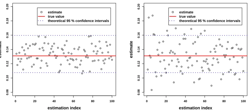
The results we obtain for 100 independent estimations for the interacting-particle method are regrouped in Figure 1. We have used N = 200 particles andT = 300 andT = 30 iterations in the HM Algorithm 2.2. Let us first interpret the results for T = 300 iterations. In this case, we observe that the estimator is empirically non-biased. Furthermore, we also plot the theoretical 95% confidence intervals for the ideal estimator with
T = +∞, that are approximately (forN large) Ip =
pexp
−1.96
r
−logp N
, pexp
1.96
r
−logp N
. We
also recall from the discussion after (1) that the events ˆp∈Ip andp∈Ipˆare approximately equivalent whenN
is large. Hence the coverage probability ofIpfor ˆpis approximately the probability thatIpˆcontainsp, which is
the practical quantity of interest. We see on Figure 1 thatIp approximately matches the empirical distribution
of the estimator ˆp. The overall conclusion of this caseT = 300 is that there is a good agreement between theory and practice. This emphasizes the validity of using the interacting-particle method of Algorithm 2.3, involving the HM algorithm, in a space that is not a subset ofRd.
In Figure 1, we also consider the case T = 30. The estimator is still empirically unbiased. However, its empirical variance is larger, so that the theoretical 95% confidence interval Ip is non-negligibly too thin. This
can be interpreted, because whenT is small, a new particle at a given conditional sampling step of Algorithm 2.3 is not independent of the N−1 particles that have been kept. Thus, one can argue that, at each step of Algorithm 2.3, the overall set of N particles has more interdependence, so that eventually the estimator has more variance. Nevertheless, on the other hand, an estimation with T = 30 is 10 times less time-consuming than an estimation withT = 300. We further discuss this trade-off problem in Section 5.3.
Finally, for this case of a probability that is not small, we have used simple Monte Carlo as a mean to estimate it quasi-exactly. We have found that the interacting-particle method 2.3 requires more computation time than the Monte Carlo method, for reaching the same accuracy. We do not elaborate on this fact, since we especially expect the interacting-particle-method to be competitive for estimating a small probability. This is the object of Section 5.1.2. For this case of a probability that is not small, we have just investigated the features of the interacting-particle method.
5.1.2. Comparison with simple Monte Carlo in a small-probability case
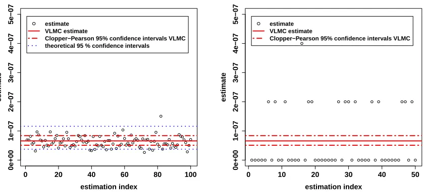
We now consider a case with possible absorption of the monokinetic particle. Thus we setP = 0.45. We keep the same valuesσ2= 1 andB = 1 as in Section 5.1.1, but we setA=−15. As a result of these parameters for
the monokinetic-particle transition kernel, the probability of interest is small. In fact, we have not estimated it with negligible uncertainty. With a simple Monte Carlo estimation of sample size 109, the probability estimate
is ¯p= 6.6×10⁻⁸. We call this estimate the very large Monte Carlo (VLMC) estimate. Given that the number
of successes in this estimate is 66, which is not very large, we are reluctant to use the Central Limit Theorem approximation for computing 95% confidence intervals. Instead, we use the Clopper-Pearson interval [6], for which the actual coverage probability is always larger than 95%. This 95% confidence interval is there equal to [5.1×10−8,8.4×10−8]. This uncertainty is small enough for the conclusions we will draw from this case. Finally, note that this very large Monte Carlo estimate is not a benchmark for the interacting-particle method, because it is much more time consuming.
For the interacting-particle method, we set N = 200 particles, and for the HM algorithm, we setT = 300 iterations. We use ˜σ2= 0.12andQ= 0.2 for the perturbation method. We still denote ˆpthe obtained estimator