A Fuzzy Realistic Mobility Model for Ad hoc
Networks
Alireza Amirshahi1, Mahmoud fathy2, Morteza Romoozi3, Mohammad Assarian4
Received (21-8-2011) Accepted (13-11-2011)
Abstract - Realistic mobility models can
demonstrate more precise evaluation results because their parameters are closer to the reality. In this paper a realistic Fuzzy Mobility Model has been proposed. This model has rules which are changeable depending on nodes and environmental conditions. It seems that this model is more complete than other mobility models. After simulation, it was found out that not only considering nodes movement as being imprecise (fuzzy) has a positive effects on most of ad hoc network parameters, but also, more importantly as they are closer to the real world condition, they can have a more positive effect on the implementation of ad hoc network protocols.
Index Terms - Mobility Model, Ad hoc Networks,
Realistic Mobility Model, Fuzzy Systems, Nodes Signal.
1-Alireza. Amirshahi is Department of Computer, Arak Branch, Islamic Azad University, Arak, Iran ( a.amirshahi@ yahoo.com)
2-Mahmoud. Fathi is Department of Computer, Tehran Branch, University Of Science and Technology, Tehran, Iran ( mahfathy@iust.ac.ir).
3-Morteza. Romoozi is Department of Computer, Kashan Branch, Islamic Azad University, Kashan, Iran. ( mromoozi@gmail.com)
4-Mohammad. Assarian is Department of Computer, Kashan Branch, Islamic Azad University, Kashan, Iran. (assarianmo@gmail.com)
I. INTRODUCTION
N
owadays ad hoc networks have been used ina variety of applications. Mobility models in ad hoc networks are of special importance. Mobility model identifies the primary place of nodes and the manner of nodes mobility. Mobility models fall into two categories: realistic and unrealistic. As realistic mobility models are more similar to real world conditions, they provide more accurate results.
Before applying to the real world, computer simulation is a valuable tool for evaluating protocols and other network parameters. Simulation can be applied easily, while implementation of ad hoc networks in the real world is difficult and expensive. Moreover, simulation has other advantages such as iterative scenario, parameter isolation, and measuring different metrics. NS2 [1] and Glomosim [2] are the most famous simulators used for evaluating and comparing computer network protocols. Mobility model, signal propagation model and routing protocol are the most important parts of wireless simulators. Many realistic models have been presented in most of which nodes mobility is random and simulation environment is free, without obstacle and pathway.
while in real world, nodes have pathways and obstacles for moving. Not only these pathways and obstacles limit their movement but also they block their signals. Meanwhile, the type of destination selection of nodes is not random. For instance, the selection of people’s destination in a university environment is not random and many parameters are involved such as time, current place, the priority of going to different places and etc.
The mobility of a mobile node and its mobility environment are not precise. Namely, a university environment is not precise because every college has different parts and precise coordination of each part cannot be stated.
As fuzzy control systems are capable of solving imprecise problems efficiently, by using fuzzy control system in the proposed Fuzzy Mobility Model, the motion rules of different kinds of nodes, based on type of the activity and environment, have been designed. Fuzzy control system includes fuzzy rules which describe the nodes mobility in an adaptable way with the environment. This model has a knowledge base which can be changed based on nodes conditions, types of nodes and environment. By using such knowledge base, the mobility rules of every environment can be imposed upon a mobility model as an input, until the mobility is created in that specific environment.
A review of the related studies has been presented in part 2. Part 3 contains the proposed Fuzzy Mobility Model. The simulator (Glomosim [5]) and its results have been presented in part 4 and the conclusion has been mentioned in part 5.
II. A REVIEW OF THE RELATED STUDIES Regarding realistic mobility models, many studies have been done, but most of them have been performed on environment model and signal blockage and just a few attention has been paid to real movement patterns. In these models, destination selection of nodes was either completely random and the selection of path by algorithm was either the shortest one or it was selected randomly which are not considered suitable. For instance, the Obstacle Mobility Model [3], presented in 2003 by A. Jardosh, is one of the most successful realistic models. This model has an appropriate signal blockage and environment sub-model and it can be used as signal blockage and environment sub-model of other models, but it lacks a real world-based
mobility pattern model. The destination selection of this model is entirely random and the path selection is done by Dijkstra algorithm with the shortest path regarding the number of edges which is not a suitable criterion.
A realistic group model, called OCGM [6], based on obstacle and mobility model RPGM [7] has been proposed which has similar environment model and blockage signal, but in its movement pattern sub-model, nodes move in groups.
Graph-based [4] is another model, environment model of which is constituted by a graph and this graph is the paths of a map and has not a specific signal blockage sub-model.
The next model which is based on Graph-based Model, named Area Graph-Graph-based [8], has been represented and its environment sub-model is similar to Graph-base Model and lacks signal blockage model, but compared to Graph-based Model, its movement pattern sub-model has been improved. In the other words as long as the nodes are inside the graph vertices, they have Random Waypoint [9] mobility. But for leaving vertex, nodes must select one of the output edges of the vertex which has probability from the beginning of simulation, along with related probability.
Still another realistic model, called Environment Aware Mobility [10] has been represented. The environment sub-model of this model is different from that of Graph-based Model mentioned above. In this mobility model, the environment is divided into a series of sub-environment inside of which there are some obstacles and movement pattern sub-model of nodes in each sub-environment can be one of the random mobility models. This model has signal blockage sub-model.
There are some realistic mobility models which touch on nodes movement pattern models. But the number of these models is by far fewer than the other models. For example, we can refer to a Cluster-based Mobility Model [11] for intelligent nodes by M.Romoozi. This mobility model has focused on the movement pattern sub-model and has improved it.
those vertices which are closer to the area of the activity with greater probability, but this selection is done by Dijkstra algorithm.
There are other models such as Manhattan Mobility Model [13], Free Way Mobility [13], and Urban Mobility Model [14]. But compared to the more complete models mentioned above, these models are of little importance.
1. Classification of Mobility Models
Mobility models can be divided into two categories: realistic and unrealistic. In realistic mobility models, the mobility of nodes is assessed in the real world conditions. In this model, not only mobility pattern of mobile nodes is considered, but also simulation environment and the effect of environment on signal nodes are examined. In unrealistic mobility models, a free and without obstacle space is taken into account in which nodes move freely everywhere and their selection of destination and path is usually random and there is no predefined obstacle and pathway for them. These models do not determine an accurate result in evaluating ad hoc network protocols.
1) Realistic Mobility Models
Realistic mobility models create an environment similar to the real world. This environment includes some pathways through which nodes must move in this pathway. This model also includes some obstacles. Not only these obstacles obstruct the nodes movement, but also they weaken or remove nodes signal. The more the environment is similar to the real world conditions, the more accurate the evaluation results will be.
Considering the analyses had done up to now, each realistic model is usually composed of 3 sub-models. These sub-models are related to one another and they can hardly be separated as follow:
-- Environment sub-model. -- Signal obstruction sub-model. -- Movement pattern sub-model.
Environment sub-model includes environmental obstacles such as buildings, mountains and etc., which usually exist in real environment. This sub-model also includes some paths that exist among these obstacles. These paths force the nodes to move only through these paths.
Signal obstruction sub-model is the effect of obstacles on nodes signal. The obstacles can
either weaken or block nodes signal, or they can pass a part of the nodes signal and block the rest. This sub-model can either consider the third dimension of obstacles or it can just consider them as two-dimensional obstacles. The type of implementation of these problems explains signal obstruction sub-model.
Movement pattern sub-model includes the manner of destination selection, the selection of path toward the destination, and the amount of pause in destination. To sum up, the manner nodes movement is explained in environment sub-model.
2. Fuzzy Control System
The term ‘fuzzy’ means imprecise. Although fuzzy systems describe uncertain and unclear phenomena, Fuzzy theory is a precise one. The heart of a fuzzy system is a knowledge base which is composed of fuzzy If-Then rules.
The main structure of fuzzy systems is shown in figure 1.
Fuzzy rules
Inference engine
DeFuzzifier Fuzzifier
Input Output
Fig. 1. The main structure of fuzzy systems.
The fuzzifier used in Fuzzy Mobility Model is a unique fuzzifier (1). This fuzzifier maps a singular point x*∈u with real value on a fuzzy
unique A` in u and the membership function in X* equals one and in other points u equals 0. It means:
=
=
′
: 0
: 1 )
(x x x*
uA
O.W (1)
w w y
y M
M
1 1 *
= − =
∑ ∑
= (2)
In this equation
y
−is the center of fuzzy
set and
w
is its hight degree and M is thenumber of our rules.
Inference engine of used in the fuzzy mobility model is multiple inference engines (3).
∏
=
= ′ ∈ =
′( ) max sup( ( ) ( ) ( ))
1
1 u x u x u y
y
u A i B
n
i A u x
M
B i (3)
III. THE PROPOSED FUZZY MOBILITY MODEL
In a real environment, nodes are divided into different groups with similar mobility features. For instance, in a university we have professor nodes, clerk nodes, and student nodes. For each group of nodes, the manner of destination selection, the movement speed, time and etc., are different.
In the real world, the destination of nodes is expressed imprecisely and the conception of fuzziness is hidden in it. For example, physical education complex includes places such as head office, volleyball saloon, and etc., and we cannot express a precise coordinates. For example, the volleyball saloon cannot be stated in unique X and Y points.
In the real world, nodes destination is selected based on the time. Namely, in a university, a professor goes to a class in the morning and to the electrical faculty at noon, but these times are not stated exactly. Some people believe that morning starts from 7 to 10, but others believe it to be from 7 to 9 and etc. So time can be considered as being fuzzy.
Regarding that each of the nodes has a different mobility, so the destination selection of each node will be different from the others. To provide an example, in a university environment, the mobility of a professor node is different from that of a student or a clerk. Therefore, their destinations are different. A professor selects a college destination, for example, while the student selects the library destination.
In the proposed Fuzzy Mobility Model, each mobile node (professor, student, and clerk) is carrying a laptop which is able to send and receive information.
1. Sub-Models of Fuzzy Mobility Model
Sub-models of Fuzzy Mobility Model include 3 parts:
1) Environment Sub-Model
Environment sub-model of Fuzzy Mobility Model is similar to Obstacle Model [3]. The environment sub-model, in Fuzzy Mobility Model, includes environmental obstacles like building, mountains and so on that exists in the real world. It also has some pathways through which nodes commute. After identifying the place of buildings and obstacles, the pathways which connect them and direct the nodes inwards and outwards the buildings are calculated by a Voronoi path calculation routine. Voronoi diagram takes the coordinates of buildings as input and then it calculates the pathways. These pathways are of equal distance to the buildings.
Fig. 2 illustrates the network scenario we have chosen for our mobility model. In fact we create a real environment to have a real simulated environment. In fig. 2, buildings have been created like rectangles. Then Voronoi diagram pathways are produced based on this model. The produced Voronoi diagram is considerably close to the real pathways around the buildings. The simulated environment can be created by using a Java tool called tergen.
In the environment sub-model, a city plan can be considered as a mobility model. This way there is no need to use Voronoi pathway calculation routine. Because the city plan contains pathways and the obstacles have been demonstrated in it.
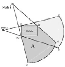
2) Signal Obstruction Sub-Model
Fig. 2. Simulation environment.
Fig. 3. Obstruction cones of nodes i and j around the obstacle [3]
3) Movement Pattern Sub-model
The manner of movement, including the path selection, destination selection, and the amount of pause in destination, will be examined in this sub-model.
In this paper, the main focus is on the movement pattern of nodes. In the proposed Fuzzy Mobility Model, firstly, nodes are divided into groups with equal mobility features. Then, the manner of destination selection of nodes is defined by using a fuzzy control system (fuzzifier, fuzzy rules, inference engine and defuzzifier). This mobility model is suitable for mobility of a mobile node which has an imprecise mobility. The pass selection method in proposed mobility model is Dijkstra shortest pass algorithm.
The proposed mobility model gains from a fuzzy control system that contains fuzzy rules. These fuzzy rules describe the node mobility in an adaptable way to the environment. Fuzzy rules express the manner of destination selection for each group of nodes. As time and place inputs are expressed imprecisely (fuzzy), it seems that Fuzzy Mobility Model is more similar to the real world than the previous realistic model and this model can be used as a part of a simulator by MANET network researchers.
In the proposed Fuzzy Mobility Model, considering fuzzy systems (fig. 1), fuzzifier
input is time and place which are expressed precisely (for example for professor node, the current place is electrical faculty and the time is 8 o’clock). Fuzifier changes these amounts from being precise into fuzzy state and they go to the inference engine along with current fuzzy rules. Afterwards, the output of the inference engine goes to the defuzzifier and the next destination is defined based on the fuzzy rules.
2. Nodes Clustering
In a university environment nodes are divided into 3 groups: professor, clerk and student. Each of these nodes has different motilities which are explained later on.
3. Mobility Analysis
Mobility analysis has different methods including locating the camera in specific places and identifying the movement of people and obtaining the related mobility model and the other method is using Radio-Frequency Identification (RFID). Still the next method is using questionnaire which has been in this mobility model. We distributed questionnaires among some university nodes and asked them to fill out the forms. This way we were able to identify the destination of these nodes in different time intervals. Because each node has different programs, the fuzziness of mobility model is proved.
4. Inputs of Fuzzy Mobility Model (university environment)
1) Time Input
Time input is divided into 3 parts: morning, noon and evening (according to fig. 4 mapped by Maple Software). A Gausian diagram has been applied to show the time as being fuzzy and its membership function has been shown in (4). x is a point in which the diagram has the highest value(1). For instance, the value of x in the morning, at noon, and in the evening can be 8, 12, and 17 respectively.
) ) ( 2 . 0 ( )
(t x a2
time
=
e
− −Time afternone none morning Fig. 4. Time input in Fuzzy Mobility Model.
Fig. 5. Places of Fuzzy Mobility Model.
2) Place Input
The other input is place which is mapped by maple software (fig. 5). In order to show the place as being fuzzy, a Gausian diagram has been used and its membership function has been shown in (5). x and y are the coordinates of the center of places and their diagram in that points has the highest value. Coordinates of the center of sites has been shown in fig. 7.
))) ) ( ) (( 10 ( ( ) ,
(xy 4 x a2 y b2 pos e− − + −
−
=
µ
(5)5. The output of the Fuzzy Mobility Model
The output of the Fuzzy Mobility Model with obstacle is the selection of destination. Considering fig. 1(the main structure of Fuzzy Systems), the inputs of mobility model are the current time and place given to the fuzzy control system (given precisely). Now regarding the given rules table, the place of destination is defined.
6. Extracting the Rules Table
As mentioned before, university nodes have different mobilities in different times. So questionnaires have been used. Fig. 6 shows a type of the forms used for each of the nodes.
Question Form Professors Clerks Students
Morning place Priority Self-service
Electrical Faculty-class Physical education -Department Library Room Mosque Technical -office Dormitory
Noon place Priority Self-service Electrical Faculty-class Physical education -Department Library Room Mosque Technical -office Dormitory
Evening place Priority Self-service
Electrical Faculty-class Physical education -Department Library Room Mosque Technical -office Dormitory
Fig. 6. Questionnaire forms of university nodes.
Questionnaire forms were submitted to 60 professors, 60 clerks, and 60 students and they were all asked to read and fill out the forms carefully. For example, the professor has to define the priority of going to the class of electrical faculty by a digit between 0 and 1 for the morning, noon, and the evening in the questionnaire. He was asked to do the same for other places in the form. When the nodes returned the questionnaire, the average of priority of each node in the morning, at noon, and in the evening was calculated and this knowledge was used for problem solving.
In order to fill out the rules table, a map of the real university environment is provided. Then, the centers of sites are defined by exact X and Y in a coordinate axis in which X and y have the maximum value of 1000. In fig. 7, the precise center of university sites is shown. For instance physical education department is located in coordinates X= 650 and Y=850.
Dormitory
×
(650,50) x 1000 Mosque
× (250,150)
Self-service
× (350,350)
Room
× (550,550)
Electrical Faculty class
× (750,650) Library
×
(450,750)
Physical education Department
×
(650,850) 1000
Technical -office
× (150,650) y
Fig. 7. Places coordinate of Fuzzy Mobility Model in university environment.
as priority of nodes for moving towards the destination sites and distance of nodes from destination sites. In (6), both parameters have been taken into account. P1 and P2 are used for defining the weight of these parameters. This is a minimum equation.
) _ ( ) 1
( 2
1
1 Max dist
d P A P k Minn
Site= = − + (6)
In this equation A is the priority of going to a place extracted from the questionnaire and d is the distance between the current place and node destination. As we have the coordinates of the center of sites, the distance between these two sites can be obtained from equation
2 2
2 1 2 1
( ) ( )
d= x −x + y −y (x1 and y1) are the
coordinates related to the current site and (x2 and y2) are the coordinates of centers of the main destinations.(Current place and destination place are the sites shown in fig. 7). The distance between two sites (d) is divided by the maximum distance (Max_dis). According to this plan the farthest distance between two places equals 806 (Max_dis=806), so the results will be a digit between 0 and 1 (6). In conclusion, the more the result d/Max_dis is, the more the distance between two sites will be.
In (6), P1 and P2 are respectively the priority of going to the destination place and giving priority to the current place rather than destination
place “0≤p1, p2≤1”. As the priority of going
to a place is more important, the value of P1 is considered equal to 0.6. Regarding the result of d/Max_dis, instead of using A, (1-A) is used to create a balance in the equation. Now, the more the result of the equation p1 (1-A) +P2 (d/Max_ dis), it points to the fact that the selection of this destination is not an appropriate choice .In each place we are, this equation must be repeated for each of other places (that can be one of the destination places) and finally the obtained figure, which has the least value, is selected as destination.
7. The Calculations Done in the University Environment
As we are in the current place and because of having 8 existing places fig. 7 in the current place, for destination selection, we should apply (6) 8 times and the selected destination will be
the result in these 8 steps. Namely, in table 1 the node is professor, so if the current place is the dormitory and the time is morning, the destination place will be electrical faculty.
Tables I, II, and III show the rules of the professor, student, and clerk nodes in Fuzzy Mobility Model.
TABLE I PROFESSOR’S RULES place
Self-service Room Self-service Room Electrical Faculty Electrical Faculty Self-service Physical education
Department Physical education
Department Physical educationDepartment Physical educationDepartment Room Library Electrical Faculty Self-service Room
Room Room Room Room
Mosque Room Mosque Dormitory Technical office Room Self-service Technical office Dormitory Electrical Faculty Dormitory Dormitory
Morning Noon Evening Time
TABLE II CLERK’S RULES place
Self-service Room Self-service Technical office Electrical Faculty Room Physical education
Department Library Physical education
Department Physical educationDepartment Physical educationDepartment Library Library Library Library Library
Room Room Room Room
Mosque Room Mosque Technical office Technical office Technical office Self-service Technical office Dormitory Room Mosque Room
Morning Noon Evening Time
TABLE III STUDENT’S RULES Place
Self-service Self-service Self-service Dormitory Electrical Faculty Electrical Faculty Electrical Faculty Electrical Faculty Physical education
Department Electrical Faculty Electrical Faculty Electrical Faculty Library Library Self-service Library Room Electrical Faculty Room Electrical
Faculty Mosque Physical education
Department Mosque Dormitory Technical office Library Self-service Library Dormitory Dormitory Mosque Dormitory
Morning Noon Evening Time
It should be mentioned that obtaining rules table has different ways. We can seek help from experts, for example, to complete the rules table.
IV. SIMULATION
The applied simulator is called Glomosim[5].
1. Simulation Parameters
we select the mobility speed of nodes between 0 m/s and 10 m/s. The stopping time will be selected randomly between 10 and 300 seconds. In different primary situations, each point of the diagram obtained from the average 20 time-simulation implementation with distributed nodes. The routing protocol is AODV.
After the primary distribution of nodes in the vertices of Voronoi graph, nodes move for 60 seconds to be distributed all over the simulation environment. Then, 20 Data Session begins. The size of the data packet is 512 byte and the rate of transfer is 4 packets per second. The maximum number of packet which can be sent in each data session is 6000. So a heap of 6000 packet can be received by 20 destinations. Twenty sources and destinations are selected randomly. During the simulation, the movement continues for a period of 3600 second. All the data sessions apply CBR traffic model (a fixed bit rate). The number of clients and servers has been selected randomly.
2. The Manner of Fuzzy Mobility Model Application to Glomosim
The formula of the fuzzy systems [15] with inference engine of multiplication, unique fuzzifier (1) and center average defuzzifier (2) will be as follow (7):
)) ( (
)) ( ( )
(
1 1
1 1
i A
n
i
M
l
i A
n
i l
M
l
x x
y
x
f
l i l i
µ µ
= =
= =
∏ ∑
∏ ∑
= (7)
n
R U
x∈ ⊂ is the input of fuzzy system and
R V x
f( )∈ ⊂ is the output of fuzzy system. In
Fuzzy Mobility Model the above mentioned formula is implemented in C language and then it is given to Glomosim simulator.
3. Evaluation Metrics
The main purpose of simulation is the examination and comparison of evaluation metrics. Fuzzy Mobility Model in the university environment is compared to other mobility models. Simulation has been done according to different speeds and now we examine the results. The evaluation metrics in the simulation done are as follow:
--Node Density: The average number of each node’s neighbors is called node
density.
--Broken Link Average: It is the average of broken links during the simulation. --Average Data packet Reception: It is the
number of receptions of the sent data packets in the desired destinations. --Routing Overhead: It is the number of
transfers of network layer controlling packets.
--End to End Delay: A delay which is required for a packet to arrive from the source to the destination.
The compared methods are as follow: --FMM (Fuzzy Mobility Model). --OMM (Obstacle Mobility Model). --CBMM (Cluster Based-Mobility Model). --RWMM (Random Waypoint Mobility Model).
4. The Results of Simulation of Fuzzy Mobility Model
1) Average Data Packet Reception
Considering fig. 8, it can be observed that average data packet reception in RWMM is better than the other methods because there are not any obstacles. In FMM, the average data packet reception is higher because nodes of the same type (for example, student node) are beside one another and have a similar working program. But in CBMM, average data packet reception is lower than FMM. Average data packet reception in OMM is lower than other models.
2) Node Density
0 10000 20000 30000 40000 50000 60000 70000
0 1 2 3 4 5 6 7 8 9 10
Pa
ck
et D
eli
ve
ry
R
atio
Speed (m\s) Average data packet Reception
OM CBMM RW FMM
Fig. 8 Average data packet reception.
0 5 10 15 20 25 30 35 40 45
0 1 2 3 4 5 6 7 8 9 10
No
de D
en
sit
y
Speed (m\s) Node Density
OM CBMM RW FMM
Fig. 9. Node density average.
0 100 200 300 400 500 600
0 1 2 3 4 5 6 7 8 9 10
Br
ok
en Li
nk
Speed (m\s) Broken Link
OM CBMM RW FMM
Fig. 10. Broken link average.
0 0.2 0.4 0.6 0.8 1 1.2
0 1 2 3 4 5 6 7 8 9 10
Av
er
ag
e E
nd
-To
-E
nd D
el
ay
Speed (m\s) End-To-End Delay
OM CBMM RW FMM
Fig. 11. End to End delay average.
3) Broken Link Average
In FMM, pathways are stable, so fewer number of links break. RWMM has a greater number of broken links and generally OMM and CBMM have a fewer number of broken links than RWMM. It can be concluded that the more is the average number of each node’s neighbors in the related mobility model, the more broken links will be. Fig. 10 illustrates broken link average.
0 10000 20000 30000 40000 50000 60000 70000 80000
0 1 2 3 4 5 6 7 8 9 10
Av
er
ag
e C
on
tr
ol
P
ac
ket
Speed (m\s) Routing Overhead
OM CBMM RW FMM
Fig. 12. Routing overhead average.
4) End to End Delay Average
In low speeds, FMM has the least end to end delay. But by raising the speed, end to end delay will be greater than OMM and CBMM. The first reason would be having different nodes which are beside one another and cannot be of the same type. Secondly, the existence of the obstacles can be the main reason why two nodes are not in the transfer range of each other. In the CBMM, end to end delay will be better because nodes are of the same type and they are clustered.
In OMM, end to end delay is better than FMM and RWMM and compared to CBMM it has noticeable changes. End to end delay average is illustrated in fig. 11.
5)Routing Overhead
Routing overhead is increased when the related mobility model has to send more controlling packets. Controlling packets are sent when pathways are not stable. From fig. 12, we can conclude that routing overhead in FMM is high primarily, but when the speed is increased, routing overhead is lower than the other mobility models. OMM has a greater routing overhead compared to FMM, because, in this model, nodes are clustered and there is this possibility that nodes beside one another not be of the same type. Finally, RWMM has the highest routing overhead, because nodes are located randomly and there are not any obstacles and all its factors such as destination selection, path selection, and movement speed are selected randomly.
5.Conclusion
of the real environment, but none of them pays any attention to the manner of nodes movement and destination selection.
Considering the examinations did up to now, each realistic model is composed of 3 sub-models: Environmental sub-model, signal obstruction sub-model and movement pattern sub-model. There is a close relationship among these sub-models. In the proposed mobility model, environmental sub-model and the signal obstruction of obstacle mobility model have been applied, but it has a different movement pattern sub-model.
A fuzzy control system containing fuzzy rules has been used in this mobility model. In this paper, it has been proved that the mobility of a mobile node is fuzzy (imprecise) and also the mobility environment is a fuzzy one. The fuzzy control system used in this paper describes node mobility in an adaptable way to the environment. These rules describe the manner of destination selection. By using a fuzzy control system in the proposed Fuzzy Mobility Model, the movement rules of different types of nodes, depending on the kind of activity and environment and so on, have been imposed. This model also has a knowledge base which is changeable depending on nodes conditions, types of nodes and the environment. Using such knowledge base, movement rules of every environment can be imposed as input on the mobility model in order to consider the movement in that environment.
The type of mobility model, number, type of arrangement, size of obstacles and the speed of nodes movement are the parameters which have a considerable effect on the simulation results.
After simulation, it was found out that most of the results in Fuzzy Mobility Model have improved. It seems that the improvement of the results is not of great importance, when it comes to realistic mobility model, it is important to be able to propose a mobility model which is more complete and precise, and is closer to the real world. As a realistic mobility model, this model can help those researchers who would like to implement ad hoc networks protocols.
REFERENCES
[1] The Network Simulator 2, http://www.isi.edu/ nsnam/ns
[2] L. Bajaj, M. Takai, R. Ahuja, K. Tang, R. Bagrodia and M. Gerla, “GlomoSim: A Scalable Network imulation Environment,” Technical Report CSD, #990027, UCLA, 1997.
[3] A. P. Jardosh, E. M. Belding-Royer, K. C. Almeroth, and S. Suri,”Towards Realistic Mobility Models for Mobile Ad Hoc Netwotks”, in Proceedings of ACM MOBICOM, San Diego, CA, 2003, pp. 217-229.
[4] j. Tian, J. Hahner, C. Becker, I. Stepanov, K. Rothermel, “Graph-based Mobility Model for Mobile Ad Hoc Network Simulation”, in the Proceedings of 35th Annual Simulatin Symposium, in cooperation with the IEEE Computer Society and ACM. San Diego, California. 2002..
[5] M. Berg, M. Kreveld, M. Overmars, O. Schwarzkopf, “ Computational Geometry: Algorithms and Applications”, Springer Verlag, 2000.
[6] J. Kristofferson, “Obstacle Constrained Group Mobility Model. “, in Department of Computer Science and Electrical Engineering Lulea University of Technology Sweden December 2005.
[7] X. Hong, M. Gerla, G., Pei, C. C. Chiang, “A Group Mobility Model for Ad hoc Wireless Networks.” In: Proceedings of the ACWIEEE MSWIM’99, Seattle, WA, pp. 53–60. August 1999.
[8] Bittner .Sven, Raffel .Wolf-Ulrich, and Scholz, “Manuel The Area Graph-based Mobility Model and its Impact on Data Dissemination Proceedings” of the 3rd Int’l Conf. on Pervasive Computing and Communications Workshops (PerCom 2005 Workshops) 2005 IEEE.
[9] Q. Zheng, X. Hong, and S. Ray, “Recent Advances in Mobility Modeling for Mobile Ad Hoc Network Research”, in ACM-SE 42 Proceedings of the 42th annual Southeast regional, Huntsville, Alabama, USA, 2004.
[10] Gang Lu, Belis Demetrios, Manson Gordon, “Study on Environment Mobility Models for Mobile Ad Hoc Network: hotspot Mobility Model and Route Mobility Model,” Wireless Com, Hawaii, USA, 2005.
[11] M. Romoozi, H. Babaei, M. Fathy, M. Romoozi. “A Cluster-Based Mobility Model for Intelligent Nodes”, in LNCS. Verlag Berlin Heidelberg, 2009, pp. 565-579.
[12] H. Babaei, M. Fathi, M. Romoozi, “Obstacle Mobility Model Based on Activity Area in Ad hoc Networks” in LNCS., Verlag Berlin Heidelberg, 2007, pp. 804-817.
[13] F. Bai, N. Sadagopan, A. Helmy, “The Important Framework For Analyzing The Impact of Mobility on Performance of Routing Protocols for Ad Hoc Networks”, in Proceedings of IEEE INFOCOM, San Francisco, CA, 2003, pp.825-832
[14] S. Marinoni, H. Kari, “Ad Hoc Routing Protocol Performance in a Realistic Environment,” In Proceeding of the Fifth IEEE International Conference on Networking (ICN 2006), Le Morne, Mauritius, April 2006.