A New Approach to Model Parameter Determination of Self-Potential Data using Memory-based Hybrid Dragonfly Algorithm

Vol.9 (2019) No. 5

ISSN: 2088-5334

A New Approach to Model Parameter Determination of Self-Potential

Data using Memory-based Hybrid Dragonfly Algorithm

Irwansyah Ramadhani

and Sungkono

Physics Department, Institut Teknologi Sepuluh Nopember, Kampus ITS Sukolilo, Surabaya, 60111, Indonesia E-mail:[email protected]; [email protected]

Abstract— A new approach based on global optimization technique is applied to invert Self-Potential (SP) data which is a highly

nonlinear inversion problem. This technique is called Memory-based Hybrid Dragonfly Algorithm (MHDA). This algorithm is proposed to balance out the high exploration behavior of Dragonfly Algorithm (DA), which causes a low convergence rate and often leads to the local optimum solution. MHDA was developed by adding internal memory and iterative level hybridization into DA which successfully balanced the exploration and exploitation behaviors of DA. In order to assess the performance of MHDA, it is firstly implemented to invert the single and multiple noises contaminated in synthetic SP data, which were caused by several simple geometries of buried anomalies: sphere and inclined sheet. MHDA is subsequently implemented to invert the field SP data for several cases: buried metallic drum, landslide, and Lumpur Sidoarjo (LUSI) embankment anomalies. As a stochastic method, MHDA is able to provide Posterior Distribution Model (PDM), which contains possible solutions of the SP data inversion. PDM is obtained from the exploration behavior of MHDA. All accepted models as PDM have a lower misfit value than the specified tolerance value of the objective function in the inversion process. In this research, solutions of the synthetic and field SP data inversions are estimated by the median value of PDM. Furthermore, the uncertainty value of obtained solutions can be estimated by the standard deviation value of PDM. The inversion results of synthetic and field SP data show that MHDA is able to estimate the solutions and the uncertainty values of solutions well. It indicates that MHDA is a good and an innovative technique to be implemented in solving the SP data inversion problem.

Keywords— memory-based hybrid dragonfly algorithm; posterior distribution model; model uncertainty; self-potential.

I. INTRODUCTION

The Self-Potential (SP) method is one of the oldest geophysical methods and is a part of passive electrical surveying methods [1], [2]. It utilizes natural potential which is caused by electrokinetic, electrochemical, and thermoelectric activities in subsurface to measure potential difference at the ground surface [3]. The SP method has been applied widely in several cases, such as archeology [4], [5], mineral and geothermal explorations [6]–[10],

contaminant detection [11], [12], landslide investigations [13], [14], embankment stability study [13], and groundwater investigations [15], [16]. Due to its relevance in those cases, interpretation of SP data is crucial. Interpretation of SP data can be classified into three groups: graphical, tomographic, and numerical approaches [17].

In numerical approach, the SP anomalies as in Figure 1 below are frequently modelled by polarized body in simple geometry forms, such as sphere, horizontal and vertical cylinder, or inclined sheet [18]. .

Several numerical approaches has been applied to interpret SP anomalies including least square methods [19]– 21], spectral analyzes [22]–[24], derivative and gradient analyzes [25], [26], moving average methods [27], [28], and global optimization methods, for example: particle swarm optimization (PSO) [29], [30], genetic algorithm (GA) [17], [30], simulated annealing (SA) [31], [30], differential evolution algorithm (DEA) [32], and black hole algorithm (BHA) [13]. These approaches are applied by researchers to obtain the suitable method which is able to find global optimum solution because the SP data inversion is a highly nonlinear inversion problem.

In this research, a new approach based on global optimization technique is implemented to invert the single and multiple SP anomalies, which are caused by spherical, cylindrical, or inclined sheet sources. This approach is called memory-based hybrid dragonfly algorithm (MHDA) [33]. This algorithm is developed from Dragonfly Algorithm (DA) and combined with PSO to solve the drawbacks of DA, i.e. low convergence rate. This drawback often leads to local optimum solution. In order to assess the performance of MHDA, it is applied for the noise contaminated in synthetic SP data because it has not been applied for this problem nor any geophysical inverse problems. Subsequently, MHDA is applied to obtain model parameters of the field SP data for several cases.

II. MATERIAL AND METHOD

A. Forward Formulation of SP Anomaly

The observed SP anomaly at point over a sphere or cylindrical anomaly (Fig. 1a and 1b) can be expressed in the following formula [34]:

(1)

where is the electrical dipole moment (mV m2q-1), is the measurement point at ground surface along the profile line (m), denotes the central coordinates of the anomaly (m),

is the depth of the anomaly’s center (m), is the polarization angle (0), and is the shape factor. The shape factors are 0.5, 1.0, and 1.5 for vertical cylinder, horizontal cylinder, and sphere respectively. Meanwhile, the SP anomaly at point on the profile line which is perpendicular to the strike of inclined sheet anomaly (Fig. 1c) can be expressed as follows [35]:

(2)

where is the half-width of inclined sheet (m). In the field observations, two or more anomalies are commonly found along a profile line, which make an interesting point for further investigation. Therefore, the multiple SP anomalies at point on profile line can be expressed in the formula below [35]:

(3)

where is anomaly at for -th body and n denotes number of anomalies.

B. Memory-based Hybrid Dragonfly Algorithm

Dragonfly algorithm (DA) is a new meta-heuristic optimization technique which is proposed by Mirjalili [36]. DA was inspired by the swarming behaviors of dragonflies, which consists of static and dynamic swarms. In the static swarm behavior, also known as hunting behavior, small groups of dragonflies moves locally and change courses abruptly to hunt preys over a small area. Meanwhile, in the dynamic swarm, also known as migratory behavior, a substantial number of dragonflies migrate over long distances in one direction. Those swarm behaviors represent the main characteristics of meta-heuristic based optimization including exploitation and exploration. The exploitation finds the best candidate for a solution in the local region, while the exploration enables solution candidates to explore search space and generate a variety of solutions [13]. A meta-heuristic algorithm must balance both characteristics to find a global optimum solution and avoid local optimum solution.

Those behaviors are modelled as interaction among dragonflies in several operators such as separation, alignment, cohesion, attraction to food, and threats of external enemies [36]. Separation operator avoids static collision of a dragonfly with other dragonflies in the neighborhood, alignment operator matches the velocity of a dragonfly to other dragonflies in the neighborhood, cohesion operator refers to the tendency of a dragonfly towards the mass center of the neighborhood, food operator attracts dragonflies towards the best solution, and enemy operator prevents dragonflies from the worst solution. Each of these operators is assigned by weight factors, which are adaptively tuned, to balance the exploration and exploitation behaviors in optimization process. Additionally, the exploration and exploitation behaviors are also guaranteed by the radii of neighborhoods, which increase proportionally to the number of iterations.

DA has been applied to geophysical inverse problems and obtained sufficiently good solution [37]. However, DA is more explorative which causes low convergence rate and often leads to the local optimum solution. The high exploration behavior of DA is caused by Levy flight process to explore search space if there is no any neighboring around a dragonflies [36]. In order to solve these drawbacks, Ranjini and Murugan [33] proposed MHDA which adapts PSO concepts including pbest and gbest, into DA. These concepts, which are known as internal momory, enable dragonflies to remember previous potential positions. Furthermore, iterative level hybridization, which executes DA and PSO in sequence, is applied to exploit promising area solution with consideration to the internal memory of DA. This process will improve the exploitation of DA and balance the high exploration characteristic of DA. Therefore, MHDA successfully balances both characteristics to achive global optimum solution.

positions. Pbest positions are obtained by comparing fitness value of current population with previous best fitness. Meanwhile, gbest position is obtained by comparing food fitness of current population with previous one. Those quantities are saved in pbest and gbest matrix. Subsequently, the internal memory is considered in the hybridization scheme. In this process, population and global best of PSO are initialized respectively by DA-pbest and DA-gbest. PSO is implemented to exploit promising areas, which is obtained from DA scheme. The velocity and position update equations of PSO in iterative level hybridization process can be expressed in the formula below:

(4)

(5)

where and are respectively two successive iterations of PSO, and denote vectors which contain respectively velocity and position components of -th particle in D dimensions space, and indicate local and global acceleration constants, and are uniformly distributed random numbers, is inertia weight, is called “personal best” of -th PSO particle, and is called “global best” of best overall swarm best solution in -th iteration for PSO.

C. SP data inversion using MHDA

In the SP data inversion problem, is the position vector, which contains model parameters of SP as in Eq. (1) or Eq. (2). For example, if the considered SP data is a sphere or horizontal anomaly, in Eq. (5) must contain model parameters including , , , , and . These model parameters are needed to calculate SP data (Eq. 1). On the other hand, if the considered SP data is inclined sheet anomaly, contains model parameters such as , , , , and (Eq. 2). If the considered SP data contains two or more anomalies, model parameters of each anomaly are needed to calculate each potential anomaly (Eq. 1 or Eq. 2) and Eq. (3) is considered to calculate total potential anomaly.

In order to obtain model parameters of SP data, MHDA is applied to minimize the difference between observed and calculated SP data which is represented by the objective function . The objective function of SP data inversion is defined by [13]:

(6)

where and represent observed and calculated SP anomaly respectively, at point on profile line. Calculated SP anomaly can be obtained by Eq. (1)-(3) which is based on the shape and number of anomaly. Furthermore, misfit between observed and calculated SP data can be evaluated by average relative error (%) with the following equation [13]:

(7)

where is the number of observed SP data.

D. Uncertainty Estimation

In geophysical data inversion problems, researchers often deal with several models which fit with the observation data. This phenomenon is known as non-uniqueness and is caused by several factors: 1) earth, where properties continuously vary in all directions, is modeled as a discrete form in the inversion process, 2) the obtained observation data is not sensitive to any earth model, and 3) the presence of noise in data can increase the degree of the uncertainty value from the obtained inversion results [38]. Therefore, in this research, statistical approach is applied to estimate solutions in posterior distribution model (PDM) terms. This approach also enables to estimate the uncertainty boundaries.

Stochastic inversion methods provide several solutions which fit to the observed data. This method is different from the deterministic inversion methods which provide only a single solution. Therefore, this method can provide PDM which contains possible model parameters for global optimum solution. The PDM is obtained from the exploration process of a global optimization algorithm in the search space [13]. All accepted models of PDM have lower misfit values than specified tolerance value of the objective function in the inversion process. Therefore, all accepted models of PDM are associated with high fitness region.

III.RESULTS AND DISCUSSION

A. Inversion of Synthetic SP Data

In order to assess the performance of MHDA, it was initially tested for the noise contaminated synthetic SP data, which depict observation data. The presence of noise in data will affect the performance of an algorithm to obtain global optimum solution. Fernández Martínez et al. in [39] stated that noise in data will deform cost function of a nonlinear problem. It means that a noisy function will reach a global optimum solution, which is not the true global optimum. It is caused by hyperquadric shifting which relates to global optimum solution. Noise in data also increases the uncertainty in inverse solutions because it is amplified to the model parameters. Furthermore, noise in data will increase local optimum solution in search space [40]. Therefore, noisy synthetic SP data is suitable to test the performance of MHDA. If the result is not at all or is only slightly affected, it can be concluded that MHDA can be implemented in field SP data.

1) Inversion of a Sphere Anomaly

The model parameters, which are used to generate SP data of sphere anomaly, are shown in Table 1. The model parameters were adopted from a research by Sungkono and Warnana [13]. In order to invert SP anomaly, initially, search space boundaries of each model parameter were determined as shown in Table I. The wide search space is used to test the performance of MHDA in exploring and exploiting the search space. In this research, the solution and the uncertainty of the solution are estimated by PDM, which is obtained from the inversion process. Sungkono and Santosa [41] stated that the solution can be estimated by means, medians, or modal values of PDM. If PDM follows Gaussian distribution, those values are almost the same. Meanwhile, the uncertainty of the solution can be estimated by the standard deviation of PDM.

TABLEI

TRUE MODEL PARAMETERS,SEARCH SPACE, AND INVERTED MODEL PARAMETERS OF A SPHERE ANOMALY

Model Parameters

True Model

Search Space Inverted Model

K (mV) -10000 -100000-100000 -10224 ± 1529

(deg) 60 -20-180 59.73 ± 0.51

z (m) 10 0-100 10.09 ± 0.28

x0 (m) 40 1-100 39.95 ± 0.14

q 1.5 0.7-1.8 1.5050 ± 0.02

Misfit - - 0.0053

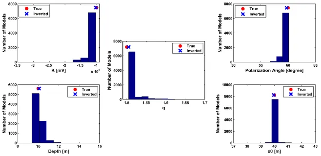
Histogram of model parameters from a sphere anomaly inversion is shown in Fig. 2.

Fig. 2 Histogram of PDM for each model parameter from a sphere anomaly inversion result

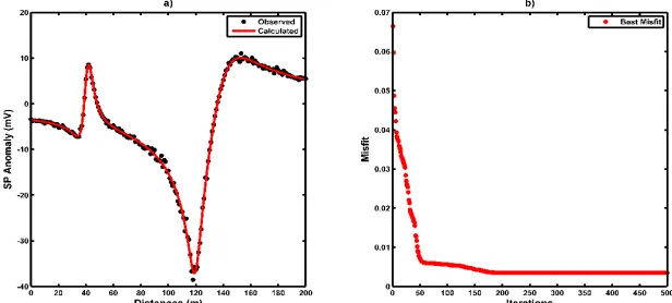
All accepted model parameters have lower misfit value than specified tolerance value, which can be determined by the best misfit curve as iteration function (Fig. 3b). In Fig. 3b, misfit curve is relatively constant below 0.05. Therefore, it is set as the tolerance value to determine PDM. The value of each PDM is represented by median value (blue cross), which is very close to the true model parameter (red dot). Furthermore, the highest frequency on the histogram correlates to the true model parameter, which can indicate the solution of the SP data inversion. Therefore, it means that the inversion result is very good. The inversion result of a sphere anomaly is shown in Table I, which is presented by

median ± standard deviation values of PDM. The median value represents the solution of a sphere anomaly inversion, while standard deviation represents the uncertainty value of the obtained solution. The uncertainty values of each inverted model parameter are sufficiently low and true model parameters lie within range of the uncertainty values. It indicates robustness of MHDA to invert the noisy sphere anomaly data. Fitted curve between observed and calculated SP data is shown in Fig. 3a which is very good with 0.0053 (0.53%) misfit value. In addition, MHDA has rapid convergence rate, which converges before 50 iterations (Fig. 3b).

2) Inversion of an Inclined Sheet Anomaly

For an inclined sheet anomaly, the model parameters are shown in Table II. The model parameters are adopted from a research of Biswas and Sharma in [42]. The wide search

space boundaries for each model parameter are also used as shown in Table II. Histogram of model parameters from an inclined sheet anomaly inversion is shown in Fig. 4.

Fig. 4 Histogram of PDM for each model parameter from an inclined sheet anomaly inversion result

All accepted models as PDM have a lower misfit value than specified tolerance value. Based on the best misfit curve as iteration function (Fig. 5b), the tolerance value is 0.05. In Fig. 4, each PDM is represented by median value (blue cross) which is very close to the true model parameter (red dot). In addition, the highest frequency of the histogram correlates to the true model parameter, which indicates that the inversion result is very good. The inversion result of an inclined sheet anomaly, which is represented by median ± standard deviation, is shown in Table II. The uncertainty values of each inverted model parameter are sufficiently low. Additionally, true model parameters lie in range of the uncertainty value. Therefore, MHDA is robust in inverting noisy inclined sheet anomaly data. The inversion result can also be assessed by curve fitting between observed and calculated an inclined sheet SP data in Fig. 5a. It shows that

very good fitted curve with 0.00613 (0.613%) misfit value. Additionally, rapid convergence rate of MHDA is shown in Fig. 5b which converges before 50 iterations.

TABLEII

TRUE MODEL PARAMETERS,SEARCH SPACE, AND INVERTED MODEL PARAMETERS OF AN INCLINED SHEET ANOMALY Model

Parameters True Model

Search Space Inverted Model

K (mV) 50 -1000-1000 48.83 ± 2.50

(deg) 30 0-180 29.74 ± 0.57

z (m) 40 0-200 38.19 ± 0.57

x0 (m) 200 0-800 198.62 ± 1.20

a (m) 50 1-100 50.93 ± 0.63

Misfit - - 0.00613

3) Inversion of Multiple Anomalies

Multiple anomalies (two or more anomalies) are commonly found in SP surveys. This problem is more interesting than single SP anomaly problem because there are more model parameters evaluated. The model parameters

for multiple anomalies (Table III) were adopted from a research of Sungkono and Warnana in [13]. The wide search space boundaries were also used for this problem as shown in Table III.

TABLEIII

TRUE MODEL PARAMETERS,SEARCH SPACE, AND INVERTED MODEL PARAMETERS OF MULTIPLE ANOMALIES

Model Parameters True Model Search Space Inverted Model

1st Body

K (mV) 500 0-1500 424.29 ± 18.25

(deg) 30 0-180 31.87 ± 0.87

z (m) 5 0-80 4.87 ± 0.22

q 1.5 0.4-1.8 1.47 ± 0.01

x0 (m) 40 0-100 40.11 ± 0.33

2nd Body

K (mV) 10 0-50 9.82 ± 0.47

(deg) 150 0-180 150.28 ± 0.74

z (m) 10 0-50 9.99 ± 0.25

a (m) 12 2-30 12.14 ± 0.33

x0 (m) 130 75-150 130.07 ± 0.33

Misfit - - 0.0035

PDM of each model parameter obtained from the inversion process are shown in Fig. 6.

Based on the best misfit curve as iterations function in Fig. 7b, tolerance value is 0.05. In Fig. 6, each PDM is represented by median value (blue cross) which is close to the true model parameter (red dot). The highest frequency of the histogram also correlates to the true model parameter, which means that the inversion result is very good for multiple anomalies problem.

The inversion result of the multiple anomalies problem is shown in Table III. The model parameters of the first anomaly body are parameters of a sphere anomaly, while the other is parameters of an inclined sheet anomaly. The

uncertainty values of inverted model parameters are sufficiently low. There are several true models, which do not lie in range of the uncertainty values; however the effect of the uncertainty value of the inverted model parameter was close to the true model parameter. Therefore, MHDA is robust for inverting noisy multiple anomalies. Fig. 7a shows that a good fitted curve between observed and inverted SP data with 0.0035 (0.35%) misfit value. Furthermore, the rapid convergence rate of MHDA is shown in Fig. 7b which converges before 200 iterations.

Fig. 6 Histogram of PDM for each model parameter from multiple anomalies inversion result. The parameters of first anomaly are upper panel and the other are lower panel.

B. Inversion of Field SP Data

MHDA has been implemented for the noise contaminated synthetic SP data inversion and the results are very good. Subsequently, MHDA is implemented for the field SP data inversion in several cases, which are adopted from several previous researches. The inversion results are also compared by previous researches to test the performance of MHDA for the field SP data inversion. For a single anomaly, MHDA uses 50 particles, 500 iterations for buried metallic drum anomaly and 300 iteration for landslide anomaly, and 200 hybridization iterations. Meanwhile, for multiple anomalies, MHDA uses 200 particles, 1000 iterations, and 200 hybridization iterations.

1) Inversion of a Buried Metallic Drum Anomaly

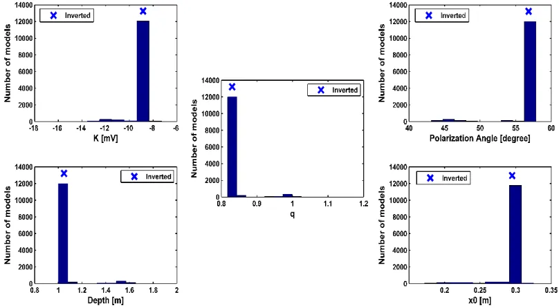
Srigutomo et al. in [43] investigated a buried metallic drum which was intentionally buried in May, 2004. It had a diameter of-0.6 m and 1.2 m in length. It was filled with metal scraps and powder. The metallic drum was buried horizontally at a depth of 2.5 m and N-S direction. After one year, SP method was carried out to measure the buried metallic drum anomaly. Several inversion methods had been applied for this problem: local [19, 43] and global [13] optimization approaches. In order to invert a buried metallic drum anomaly data, wide search space boundaries were used as shown in Table IV.

TABLEIV

SEARCH SPACE AND INVERTED MODEL PARAMETERS OF A BURIED METALLIC DRUM ANOMALY FROM SEVERAL APPROACHES

Histogram of accepted model parameters from a buried metallic drum anomaly inversion is shown in Fig. 8.

Table IV. This result is compared with several previous researches (Table IV). It shows that the obtained result is sufficiently close to other results, which indicates horizontal cylinder anomaly (q _≈ 1). Additionally, the other parameters

were also close to the previous research results. The highest frequency of histogram is also sufficiently close to the previous researches. Furthermore, Fig. 9a shows a good fitted curve between observed and inverted a buried metallic

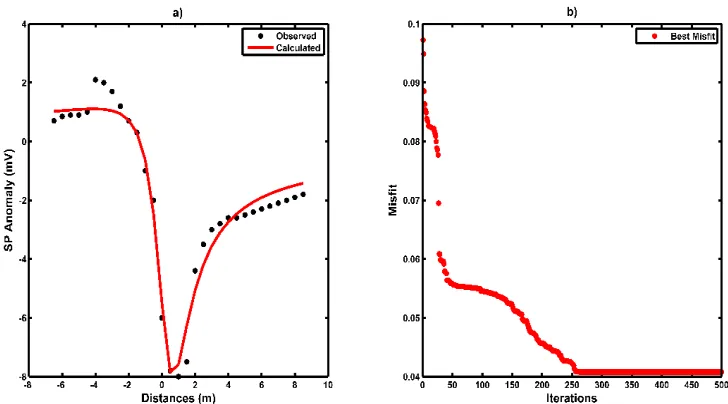
drum anomaly with 0.041 (4.1%) misfit value. Meanwhile, Fig. 9b shows that MHDA converges before 280 iterations. In Fig. 9b, the best misfit curve is relatively constant below 0.05. Therefore, this value is set as the tolerance value. The inversion result of a buried metallic drum anomaly represented as median ± standard deviation is shown in Inversion of a Landslide Anomaly

Model Parameters Search Space of MHDA Inverted Model

Srigutomo et al. [43] Chandra et al. [19] Sungkono and Warnana [13] MHDA

K (mV) -1000-1000 -10.733 -10.7308 -9.09 ± 0.20 -8.8514 ± 0.65

(deg) 0-180 45.78 44.3241 55.21 ± 1.59 56.8157 ± 2.30

z (m) 0-100 1.234 1.2325 1.15 ± 0.13 1.05 ± 0.10

q 0.3-1.8 0.916 0.9225 0.8 ± 0.0 0.83 ± 0.03

x0 (m) -6.5-8.5 - - 0.25 ± 0.04 0.30 ± 0.02

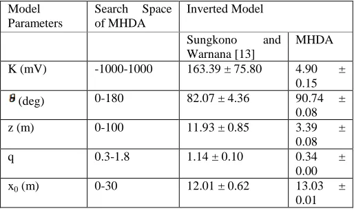
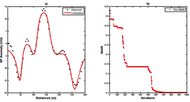
Sungkono and Warnana [13] investigated the causes of a landslide which occurred in Sawoo district area, Ponorogo regency, East Java, Indonesia on April 12th, 2017 with SP method. The main causal factor of the landslide in the area was water accumulation in rocks, which caused deformation. The deformation can be observed by the appearance of scarp on the surface. Meanwhile, the source of anomaly can be observed by SP data. In order to invert a landslide anomaly data, wide search space boundaries were used as shown in Table V. The inversion result of a landslide anomaly data is shown in Table V. Histogram of accepted model parameters from a landslide anomaly inversion are shown in Fig. 10. Fig. 11b shows that the best misfit curve is relatively constant of below 0.04. Therefore, this value is set as the tolerance value.

TABLEV

SEARCH SPACE AND INVERTED MODEL PARAMETERS OF A LANDSLIDE ANOMALY FROM SEVERAL APPROACHES

Fig. 10 Histogram of PDM for each model parameter from a landslide anomaly inversion result Model

Parameters

Search Space of MHDA

Inverted Model Sungkono and

Warnana [13]

MHDA K (mV) -1000-1000 163.39 ± 75.80 4.90 ± 0.15

(deg) 0-180 82.07 ± 4.36 90.74 ±

0.08 z (m) 0-100 11.93 ± 0.85 3.39 ± 0.08

q 0.3-1.8 1.14 ± 0.10 0.34 ± 0.00

x0 (m) 0-30 12.01 ± 0.62 13.03 ± 0.01 Fig. 9 Fitting curve between observed and calculated (a) and best misfit curve as iterations function (b) for the

Fig. 11 Fitting curve between observed and calculated (a) and best misfit curve as iterations function (b) for the inversion result of a landslide anomaly

This result is also compared by previous research. It shows that the obtained result is different but the center coordinates of anomaly (xo) is close to the previous research.

The result obtained by MHDA is close to vertical cylinder anomaly (q _≈ 0.5), while horizontal cylinder is obtained by

previous research. However, the obtained result by MHDA is supported by a research from Ramadhany et al. [44] which implemented Microtremor method in the area. The research focused on calculating the slope stability with vulnerability index (Kg). Furthermore, Principal Component Analysis (PCA) examined the properties of particle motion. Particle motion analysis showed that the source of vibration in the area was dominated by vertical motion. It was caused by fluid in overburdened pores of rocks. Fig. 11a shows that a good fitted curve between observed and inverted a landslide anomaly data with 0.0294 (0.294 %) misfit value. Further, Fig. 9b shows that MHDA converges before 100 iterations.

2) Inversion of Lumpur Sidoarjo (LUSI) Embankment Anomalies

Sungkono and Warnana in [13] investigated the stability of LUSI embankment with SP method on 11th – 20th July 2016. LUSI embankment was built to control the spreading hot mudflow at Porong, Sidoarjo. It is an earth-filled embankment composed of pebble-soil materials [45]. Additionally, it lies on soft grounds, which is composed of uncompacted clay and silt soils. Therefore, LUSI embankment faces three types of embankment failures: hydraulic, seepage, and structural failures [46]. Additionallya, LUSI embankment area is controlled by two faults: Watukosek and Siring faults [13]. These faults system can deform the LUSI embankment. The search space boundaries of each parameter and the result of LUSI embankment anomalies inversion are shown in Table VI.

The result is also compared with a previous research in the area. The inversion result of MHDA indicates that first anomaly body is close to vertical cylinder anomaly (q _≈ 0.5)

and the other is close to horizontal cylinder anomalies (q ≈

1). Meanwhile, the inversion result of Sungkono and Warnana [13] indicates that all of the anomaly bodies are horizontal cylinders. Furthermore, the center of anomalies obtained by MHDA is relatively close to the previous research.

TABLEVI

SEARCH SPACE AND INVERTED MODEL PARAMETERS OF LUSI EMBANKMENT ANOMALIES FROM SEVERAL APPROACHES

The vertical cylinder anomaly obtained by MHDA is supported by the research of Husein et al. in [47] which indicates a piping phenomenon. The piping is caused by saturated embankment and it affects the stability of an embankment above 11 m in depth. Meanwhile, the horizontal cylinder anomalies indicates seepage phenomenon. The occurring seepage was caused by penetration of mud fluid through LUSI embankment. Fig. 12a shows good fitted curve between observed and calculated LUSI embankment anomalies data with 0.20147 misfit value. Convergence rate of MHDA for this problem is lower than previous problem because more model parameters were evaluated.

Model Parameters

Search Space of MHDA

Inverted Model

Sungkono and Warnana [13]

MHDA

K (mV) -1000-1000 163.39 ± 75.80 4.90 ± 0.15

(deg) 0-180 82.07 ± 4.36 90.74 ±

0.08

z (m) 0-100 11.93 ± 0.85 3.39 ±

0.08

q 0.3-1.8 1.14 ± 0.10 0.34 ±

0.00

x0 (m) 0-30 12.01 ± 0.62 13.03 ±

Fig. 12 Fitting curve between observed and calculated (a) and best misfit curve as iterations function (b) for the inversion result of LUSI embankment anomalies

IV.CONCLUSIONS

A new approach based on global optimization technique, Memory-based Hybrid Dragonfly Algorithm (MHDA), has been implemented to solve highly nonlinear SP data inversion problem, which is caused by simple geometry, bodies, such as sphere, cylinder, and inclined sheet. In this research, MHDA is initially tested for the noise contaminated synthetic SP data for single and multiple anomalies. Furthermore, MHDA is implemented to invert SP data of a buried metallic drum, a landslide, and LUSI embankment anomalies. Both inversion results show that MHDA is able to provide Posterior Distribution Model (PDM), which is used to estimate solutions via median values and model uncertainties via standard deviation values of PDM. For the synthetic data, the estimated solutions are close to the true models. Additionally, true models lie in range of the uncertainty value. It indicates that MHDA is robust for inverting noisy SP data. Subsequently, for the field data, MHDA is able to obtain solutions, which have good correspondence with previous research results. Moreover, MHDA is able to solve inversion problem of LUSI embankment anomalies, which are complex problems. Therefore, MHDA is an innovative technique to solve the SP data inversion problem.

REFERENCES

[1] M. S. Roudsari and A. Beitollahi, “Forward modelling and inversion of self-potential anomalies caused by 2D inclined sheets,” Exploration Geophysics., vol. 44, no. 3, pp. 176-184, 2013. [2] P. Kearey, M. Brooks, and I. Hill, An introduction to geophysical

exploration, 3rd ed., Malden, MA: Blackwell Science, 2002. [3] W. M. Telford, L. P. Geldart, and R. E. Sheriff, Applied Geophysics,

2 ed., Cambridge: Cambridge University Press, 1990.

[4] J. C. Wynn and S. I. Sherwood, “The Self-Potential (SP) Method: an Inexpensive Reconnaissance and Archaeological Mapping Tool,” J. Field Archaeol., vol. 11, no. 2, pp. 195–204, Jan. 1984.

[5] M. G. Drahor, “Application of the self-potential method to archaeological prospection: some case histories,” Archaeol. Prospect., vol. 11, no. 2, hlm. 77–105, Apr. 2004.

[6] S. A. Sultan, S. A. Mansour, F. M. Santos, and A. S. Helaly, “Geophysical exploration for gold and associated minerals, case study: Wadi El Beida area, South Eastern Desert, Egypt,” J. Geophys. Eng., vol. 6, no. 4, pp. 345–356, Dec. 2009.

[7] H. Ramazi, M. R. H. Nejad, and A. A. Firoozi, “Application of integrated geoelectrical methods in Khenadarreh (Arak, Iran) graphite deposit exploration,” J. Geol. Soc. India, vol. 74, no. 2, pp. 260–266, 2009.

[8] Y. Kawada dan T. Kasaya, “Marine self-potential survey for exploring seafloor hydrothermal ore deposits,” Sci. Rep., vol. 7, no. 1, Dec 2017.

[9] R. F. Corwin dan D. B. Hoover, “The self-potential method in geothermal exploration,” Geophysics, vol. 44, no. 2, pp. 226–245, 1979.

[10] S. A. Mehanee, “Tracing of paleo-shear zones by self-potential data inversion: case studies from the KTB, Rittsteig, and Grossensees graphite-bearing fault planes,” Earth Planets Space, vol. 67, no. 1, pp. 14, 2015.

[11] G. O. Emujakporue, “Self Potential Investigation of Contaminants in a Dumpsite, University of Port Harcourt, Nigeria,” World Sci. News, vol. 57, pp. 140–148, 2016.

[12] P. Soupios and M. Karaoulis, “Application of Self-Potantial (SP) Method for Monitoring Contaminants Movement,” 2015.

[13] Sungkono and D. D. Warnana, “Black hole algorithm for determining model parameter in self-potential data,” J. Appl. Geophys., vol. 148, pp. 189–200, Jan. 2018.

[14] D. Kušnirák, I. Dostál, R. Putiška, and A. Mojzeš, “Complex geophysical investigation of the Kapušany landslide (Eastern Slovakia),” Contrib. Geophys. Geod., vol. 46, no. 2, pp. 111–124, Jun. 2016.

[15] A. Jardani, A. Revil, W. Barrash, A. Crespy, E. Rizzo, S. Straface, M. Cardiff, B. Malama, C. Miller, and T. Johnson, “Reconstruction of the Water Table from Self-Potential Data: A Bayesian Approach,” Ground Water, vol. 47, no. 2, pp. 213–227, Mar. 2009.

[16] T. Goto, K. Kondo, R. Ito, K. Esaki, Y. Oouch, Y. Abe, and M. Tsujimura, “Implications of Self-Potential Distribution for Groundwater Flow System in a Nonvolcanic Mountain Slope,” Int. J. Geophys., vol. 2012, hlm. 1–10, 2012.

[17] R. Di Maio, P. Rani, E. Piegari, and L. Milano, “Self-potential data inversion through a Genetic-Price algorithm,” Comput. Geosci., vol. 94, pp. 86–95, Sep. 2016.

[18] H. M. El-Araby, “A new method for complete quantitative interpretation of self-potential anomalies,” J. Appl. Geophys., vol. 55, no. 3–4, pp. 211–224, Mar. 2004.

[19] A. D. Candra, W. Srigutomo, Sungkono, and B. J. Santosa, “A complete quantitative analysis of self-potential anomaly using singular value decomposition algorithm,” in Proc. IEEE ICSIMA, 2014, p. 1–4.

[20] M. Dehbashi and M. M. Asl, “Determining Parameters of Simple Geometric Shaped Self–potential Anomalies,” Indian J. Sci. Technol., vol. 7, no. 1, pp. 79–85, 2014.

[21] K. Essa, S. Mehanee, and P. D. Smith, “A new inversion algorithm for estimating the best fitting parameters of some geometrically simple body to measured self-potential anomalies,” Explor. Geophys., vol. 39, no. 3, pp. 155-163, 2008.

Quantitative Interpretation,” Int. J. Geophys., vol. 2012, pp. 1–8, 2012.

[23] R. Di Maio, E. Piegari, P. Rani, and A. Avella, “Self-Potential data inversion through the integration of spectral analysis and tomographic approaches,” Geophys. J. Int., vol. 206, no. 2, pp. 1204– 1220, 2016.

[24] G. Mauri, G. Williams-Jones, and G. Saracco, “MWTmat— application of multiscale wavelet tomography on potential fields,” Comput. Geosci., vol. 37, no. 11, pp. 1825–1835, 2011.

[25] E. M. Abdelrahman, A. G. Hassaneen, and M. A. Hafez, “Interpretation of self-potential anomalies over two-dimensional plates by gradient analysis,” Pure Appl. Geophys., vol. 152, no. 4, pp. 773–780, 1998.

[26] E. M. Abdelrahman, H. M. El‐Araby, A. G. Hassaneen, and M. A. Hafez, “New methods for shape and depth determinations from SP data,” GEOPHYSICS, vol. 68, no. 4, pp. 1202–1210, Jul. 2003. [27] E. M. Abdelrahman, K. S. Essa, E. R. Abo-Ezz, and K. S. Soliman,

“Self-potential data interpretation using standard deviations of depths computed from moving-average residual anomalies,” Geophys. Prospect., vol. 54, no. 4, pp. 409–423, 2006.

[28] E. M. Abdelrahman, T. M. El-Araby, and K. S. Essa, “Shape and depth determinations from second moving average residual self-potential anomalies,” J. Geophys. Eng., vol. 6, no. 1, pp. 43–52, Mar. 2009.

[29] F. A. Monteiro Santos, “Inversion of self-potential of idealized bodies’ anomalies using particle swarm optimization,” Comput. Geosci., vol. 36, no. 9, pp. 1185–1190, Sep. 2010.

[30] G. Göktürkler dan ç Balkaya, “Inversion of self-potential anomalies caused by simple-geometry bodies using global optimization algorithms,” J. Geophys. Eng., vol. 9, no. 5, pp. 498–507, Oct. 2012. [31] S. P. Sharma and A. Biswas, “Interpretation of self-potential anomaly

over a 2D inclined structure using very fast simulated-annealing global optimization — An insight about ambiguity,” GEOPHYSICS, vol. 78, no. 3, pp. WB3-WB15, May. 2013.

[32] X. Li and M. Yin, “Application of Differential Evolution Algorithm on Self-Potential Data,” PLoS ONE, vol. 7, no. 12, pp. e51199, Dec. 2012.

[33] K. S. Sree Ranjini and S. Murugan, “Memory based Hybrid Dragonfly Algorithm for numerical optimization problems,” Expert Syst. Appl., vol. 83, pp. 63–78, Oct. 2017.

[34] B. B. Bhattacharya and N. Roy, “A note on the use of a nomogram for self-potential anomalies,” Geophys. Prospect., vol. 29, no. 1, pp. 102–107, 1981.

[35] A. Biswas and S. P. Sharma, “Resolution of multiple sheet-type structures in self-potential measurement,” J. Earth Syst. Sci., vol. 123, no. 4, pp. 809–825, 2014.

[36] S. Mirjalili, “Dragonfly algorithm: a new meta-heuristic optimization technique for solving single-objective, discrete, and multi-objective

problems,” Neural Comput. Appl., vol. 27, no. 4, pp. 1053–1073, May. 2016.

[37] I. Ramadhani, S. Sungkono, and H. Grandis, “Comparison of Particle Swarm Optimization, Genetic, and Dragonfly Algorithm to Invert Vertical Electrical Sounding,” in EAGE-HAGI 1st Asia Pacific Meeting on Near Surface Geoscience and Engineering, 2018. [38] M. K. Sen and P. L. Stoffa, Global optimization methods in

geophysical inversion, Second edition. Cambridge, New York: Cambridge University Press, 2013.

[39] J. L. Fernández Martínez, M. Z. Fernández Muñiz, and M. J. Tompkins, “On the topography of the cost functional in linear and nonlinear inverse problems,” GEOPHYSICS, vol. 77, no. 1, pp. 1–20, Jan. 2012.

[40] J. L. F. Martínez, E. G. Gonzalo, Z. F. Muñiz, G. Mariethoz, and T. Mukerji, “Posterior Sampling using Particle Swarm Optimizers and Model Reduction Techniques:,” Int. J. Appl. Evol. Comput., vol. 1, no. 3, pp. 27–48, Jul. 2010.

[41] Sungkono and B. J. Santosa, “Differential evolution adaptive metropolis sampling method to provide model uncertainty and model selection criteria to determine optimal model for Rayleigh wave dispersion,” Arab. J. Geosci., vol. 8, no. 9, pp. 7003–7023, Sep. 2015. [42] A. Biswas and S. P. Sharma, “Optimization of self-potential

interpretation of 2-D inclined sheet-type structures based on very fast simulated annealing and analysis of ambiguity,” J. Appl. Geophys., vol. 105, pp. 235–247, Jun. 2014.

[43] W. Srigutomo, E. Agustine, and M. H. Zen, “Quantitative Analysis of Self-Potential Anomaly: Derivative Analysis, Least-Squares Method and Non-Linear Inversion,” Indones. J. Phys., vol. 17, no. 2, pp. 49–55, 2006.

[44] B. Ramadhany, S. Sungkono, A. Rohman, D. D. Warnana, and S. Lestari, “Comprehensive Analysis of Microtremor data to identify potential landslide (Study Case: KM23 Ponorogo-Trenggalek Road),” in EAGE-HAGI 1st Asia Pacific Meeting on Near Surface Geoscience and Engineering, 2018.

[45] D. S. Agustawijaya and Sukandi, “The Stability Analysis of the Lusi Mud Volcano Embankment Dams using FEM with a Special Reference to the Dam Point P10. D,” Civ. Eng. Dimens., vol. 14, no. 2, pp. 100–109, 2012.

[46] Sungkono, A. Husein, H. Prasetyo, A. S. Bahri, F. A. Monteiro Santos, and B. J. Santosa, “The VLF-EM imaging of potential collapse on the LUSI embankment,” J. Appl. Geophys., vol. 109, pp. 218–232, Oct. 2014.