A NUMERICAL SIMULATION OF TWO-PHASE FLOW INSTABILITIES
IN A TRAPEZOIDAL MICROCHANNEL
Yun Whan Na
*, J. N. Chung
†Department of Mechanical and Aerospace Engineering, University of Florida, Gainesville, FL 32611
A
BSTRACTFlow instabilities of convective two-phase boiling in a trapezoidal microchannel were investigated. using a three-dimensional numerical model. Parameters such as wall temperature and inlet pressure that characterize the instability phenomena of flow boiling with periodic flow patterns were studied at different channel wall heat fluxes and flow mass fluxes. Results were obtained for various wall heat flux levels and mass flow rates. The numerical results showed that large amplitude and short period oscillations for wall temperature and inlet pressure fluctuations are major characteristics of flow instability. The wall temperature fluctuations are mainly initiated by the transition from bubbly to slug flow patterns. Pressure fluctuations at the channel inlet and outlet were shown to be induced by the alternating flow patterns between bubbly and elongated slug flow. It was also noted that the amplitude and oscillation period of the inlet pressure fluctuations are strongly affected by the increased wall heat flux. Stable and unstable cases were identified by the different phase change numbers as the three cases invested all fit correctly in the flow boiling stability map.
Keywords: Two-phase flow, boiling heat transfer, thermal-fluid instability, microchannel, numerical simulation, volume of fluid method
1.
INTRODUCTION
Fluid flow and heat transfer in microscale channels have been used in many applications, including microchannel heat sinks, micro heat exchanger, and microfluidic devices. Especially, two-phase microchannel heat sinks are widely studied due to their very high heat removal performance with a large surface area to volume ratio, compact dimensions, and low flow rate requirements. For these reasons, numerous studies of two-phase flow boiling in microchannels have been extensively reported in the last decades; the studies, however, were mainly limited to experimental works (Bowers and Mudawar, 1994a; Coleman and Garimella, 1999; Zhao and Bi, 2001; Qu and Mudawar, 2003a and 2003b; Kuo et al., 2006). Hence, there is a need to numerically analyze two-phase flow boiling through a microchannel which would help us better analyze the available experimental data and also understand the heat transfer mechanism of two-phase flow boiling such as vaporization through the liquid-vapor interface in liquid thin films and bubble dynamics dealing with nucleate boiling and bubble-bubble interaction.
The flow pattern transition from bubbly flow to slug flow causes undesired flow instabilities. Two-phase flow instabilities lead to dryout and mechanical failure due to wall temperature fluctuations related with flow pattern transition. They can be also observed in microchannels as in macrochannels. The flow instabilities are very complicated because several effects such as density wave oscillation, pressure drop and temperature fluctuation occur simultaneously during flow boiling (Boure et al., 1973; Tadrist, 2007; Kakac and Bon, 2008). Recently, these flow instabilities in microchannels have been studied by several authors (Brutin et al., 2003; Brutin and Tadrist, 2004; Qu and Mudawar, 2004; Wu and Cheng, 2004; Hetsroni et al., 2005; Muwanga et al., 2007; Wang
* Currently at Samsung Company, South Korea † Corresponding author. Email: [email protected]
et al, 2007; Huh et al., 2007). Their investigations are quite constrained in experimental works and more comprehensive study is still needed to investigate the fundamental issues of flow instabilities to provide safe operating conditions of two-phase flow boiling in microchannels. In this work, three-dimensional numerical modeling of flow boiling in a trapezoidal microchannel is performed to analyze the flow instabilities. Through the current study, an alternative predictive method to avoid an experimental error which can occur by experimental works will be provided to determine stable and unstable flow boiling regimes.
1.1 Two-Phase Flow Instabilities
1.1.1 Static and Dynamic Flow Instabilities
Two-phase flow instabilities leading to mechanical damage and system control problems are observed in many thermal management systems using forced or natural convection boiling in a heated channel. Their mechanistic behavior is very complicate due to simultaneous interactions between channel geometries and flow conditions such as subcooled liquid, mass flux, heat flux, and inlet pressure (Qu and Mudawar, 2003a; Wu and Cheng, 2003c and 2004). Flow instabilities are important factors for providing thermal safety limits for two-phase systems under certain operating conditions.
Flow instabilities are categorized as static and dynamic instability (Bergles, 1981). Static instabilities are related to the steady-state characteristics of boiling system. It may change the boiling system to a different steady-state operating condition or lead to a cyclic oscillating behavior relative to flow excursion, boiling crisis, and flow pattern transition. The periodic oscillation is caused by a small perturbation. Thus, the steady-state system tends to be unstable under specific flow conditions. Dynamic instabilities are caused by simultaneous interaction between density change, mass flux, and pressure drop. Rapid vapor
Frontiers in Heat and Mass Transfer
bubble generation in boiling system causes oscillations in relation with dynamic instabilities: density wave, pressure drop, thermal, and acoustic oscillations. Two-phase flow instabilities are briefly reviewed in this section. More detailed information for flow instabilities can be found in review papers Boure et al. (1973), Bergles (1981) and Kakac and Bon (2008) for macrochannels, Tadrist (2007) for narrow channels, and Cheng and Wu (2006) for minichannels and microchannels.
Static Instability
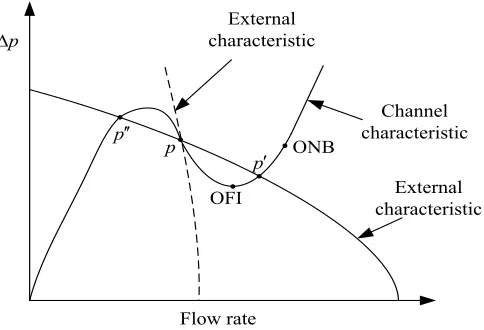
Ledinegg (1938) first observed the flow instability in two-phase boiling systems. Ledinegg (1938) instability with flow excursion, is characterized by a sudden change in low mass flow rates. It may be observed when the slope of pressure drop (channel characteristic curve) is negative and steeper than external characteristic curve with increasing mass flow rate as shown in Fig. 1 where “ONB” indicates the onset of nucleate boiling. ONB is the prerequisite for boiling instability. The portions having negative gradients of the pressure drop can be unstable. More pressure drop to sustain the flow results from a small negative disturbance to a lower flow. It leads to a shift to point p′′ when the flow rate decreases. The part of minimum pressure drop on the channel characteristic curve is referred to as the onset of flow instability (OFI) (Ghiaasiaan, 2008). Further decrease in the mass flow rate may lead to an increasing pressure drop beyond the OFI point. Steady-state operation requires that the external and channel characteristic values be the same:
, ,
p p p′ ′′. Points p and p′ are stable because a perturbation in the flow rate at these points cause an imbalance between the channel and external characteristic curves. It tends to bring the system back to the original steady state. Point p′′ is unstable. When the system operates at point
p′′, a small positive perturbation leads the system to the stable and steady condition p′; a small negative perturbation in the flow rate, however, moves to the point p′′, the stable and steady condition. Kakac and Bon (2008) and Ghiaasiaan (2008) proposed the slope of the external characteristic curve be steeper than that of the internal and/or the external characteristic curve is nearly a vertical line to avoid Ledinegg instability. Flow pattern transition instability results from cyclic flow pattern transition and flow rate variations mainly due to different pressure drop characteristics caused by various flow patterns (Boure et al.1973; Kakac and Bon, 2008). Flow pattern may change from bubbly flow to slug/annular flow when the void fraction increases if the flow rate reduces slightly from the operating point due to the result of a small perturbation. The pressure drop in the slug/annular flow is less than that in bubbly flow. That may cause the flow to increase and the void fraction may reduce. As a result, the flow pattern changes again to bubbly flow. It is similar to the flow excursion referred to as the Ledinegg (1938) instability. Nayak et al. (2003) studied the flow pattern transition instability in a natural circulation heavy water reactor. They developed a mathematical model to analyze the flow pattern transition instability and used the drift flux model to estimate the void fraction in the two-phase region. Their results showed that the instability occurs at a higher power than the Ledinegg (1938) instability and increases with a decrease in pressure or an increase in inlet subcooling.
Dynamic Instability
Dynamic instabilities occur if there is a sufficient interaction and delayed feedback between thermal or hydrodynamic inertia and compressibility of the two-phase mixture or other feedback effects among flow rate, pressure drop and density change as a result of the vapor generation in a heated channel. Static instabilities may be on the threshold of these instabilities. The dynamic instabilities can be classified as: density wave oscillations, pressure drop oscillations, thermal oscillations, and acoustic oscillations.
Fig. 1Ledinegg instability based on pressure difference and mass flow rate (Kakac and Bon (2008)).
Density wave oscillations are among the most common instabilities in two-phase flow boiling channels. These oscillations occur due to the result of phase lag and feedback among the flow rate, the pressure drop, and the vapor generation rate. When boiling takes place in heated channels, a decrease in mass flow rate leads to an increase in enthalpy of the fluid and in turn a decrease in the fluid density due to the increasing residence time in the heated channels. The propagation time of the pressure drop disturbance is much faster than that of the fluid enthalpy and density. As a result, the phase lag will be induced between the pressure drop and the inlet flow. It can lead to the oscillations of the inlet mass flow rate. The characteristics of the oscillations show low frequencies ( ~ 1 Hz); it is related to the residence time of the fluid in the channel (Tardist, 2007).
The interaction between the heated channel and the compressible volume of the heated wall can lead to pressure drop oscillations (Stenning, 1964). Boure et al. (1973) proposed that pressure wave oscillations were observed in subcooled boiling, bulk boiling, and film boiling. They also suggested that induced flow oscillations may lead to mechanical damages or system control problems. These oscillations occur when the pressure drop decreases with increasing flow rate. The frequencies of these oscillations are very low ( < 0.1 Hz).
Thermal oscillations can occur when the wall temperature highly fluctuates due to flow pattern transition (Stenning, 1964; Kakac et al., 1990). These oscillations lead to large-amplitude wall temperature oscillations and in turn cause dryout in boiling. In addition, they can deteriorate the local heat transfer performance causing wall temperature fluctuations or critical heat flux. Kakac et al. (1990) also studied the effect of inlet subcooling on two-phase flow dynamic instabilities in vertical and horizontal channels having 7.5 mm I.D. They observed that the thermal oscillations accompany the pressure drop oscillations and both are in phase; the magnitude of the pressure drop oscillations is always larger than that of the wall temperature oscillations.
1.1.2 Microchannel Forced Convection Flow Boiling
Instabilities
Two-phase flow instabilities in macrochannels were extensively studied by a number of researchers in the past decades. Yadigaroglu (1981) pointed out that two-phase flow instabilities induced by unstable flow patterns, particularly slug flow, may amplify flow disturbances and lead to a boiling crisis and mechanical damage. These instabilities may also occur in minichannels and microchannels as the channel size decreases and the imposed heat flux increases under flow boiling.
p ∆
Flow rate p′′
p
p′
External characteristic
Channel characteristic External
characteristic
OFI
Dynamic flow boiling instability in microchannels has been experimentally studied by several researchers in recent years. Kandlikar et al. (2001) observed the flow patterns of boiling in six rectangular parallel channels with 60 mm long and 1 mm hydraulic diameter. Severe pressure oscillations with around 1 Hz frequencies were investigated when boiling in the channels takes place. Reverse flows were also observed due to the growth of slug bubbles in the microchannels. Hetsroni et al. (2002) performed experiments on flow boiling of water in 21 silicon triangular microchannels with a base of 250 m. They
investigated periodic pressure drop and outlet temperature oscillations as a result of vapor generation in the parallel microchannels. They noted that the fluctuations of the wall temperature correspond to that of the pressure drop. Their results, also, showed that the amplitude and frequency of the pressure drop and wall temperature oscillations increases while the heat flux and the vapor quality increase. Qu and Mudawar (2003a and 2004) observed experimentally the pressure drop oscillations with large-amplitude and parallel channel instabilities in 21 parallel rectangular microchannels with 231 μm wide and 713 μm high. They identified severe pressure drop oscillation and mild parallel channel instability. The results showed that the severe pressure drops caused by interaction between vapor generation and compressible volume in the flow loop upstream are periodic and large amplitude oscillations. The mild parallel channel instability produced mild flow fluctuations. The instability is the result of density wave oscillation within each channel and feedback interaction between channels. They noted that the severe pressure drop oscillations may trigger pre-mature critical heat flux. Brutin et al. (2003) investigated two-phase flow instabilities in a
rectangular microchannel with a hydraulic diameter of 889 μm using n
-pentane as the working fluid. They observed two types of behavior: a steady state characterized by pressure drop fluctuations with low amplitudes (from 0.5 to 5 kPa/m) and with no characteristic frequency; an unsteady state with high amplitudes (from 20 to 100 kPa/m) and frequencies ranging from 3.6 to 6.6 Hz. The steady and unsteady behaviors are governed by the two control parameters: heat flux and flow velocity. The influence of the inlet condition on two-phase flow instability in a rectangular minichannel of 0.5×4 mm2 was observed by Brutin and Tadrist (2004). They found steady and unsteady behaviors that depend on the upstream boundary conditions: a constant velocity at the minichannel entrance and at the syringe outlet. The pressure drop fluctuations with relatively small amplitudes and higher frequencies between 6 and 18 Hz were observed, when a damper was not connected. Wu and Cheng (2003 and 2004) carried out experimental investigation on flow boiling of water in parallel trapezoidal silicon microchannels with a hydraulic diameter of 82.8 μm, 158.8 μm, and 185.6 μm, respectively. They first observed three kinds of oscillatory flow boiling modes in microchannels: liquid/two-phase alternating flow (LTAF) at low heat flux and high mass flux, continuous two-phase flow (CTF) at medium heat flux and low mass flux, and liquid/two-phase/vapor alternating flow (LTVAF) at high heat flux and low mass flux. For the LTAF case, a bubbly flow pattern was dominant and a period of oscillations was 15.6s. The amplitudes of wall temperature and inlet pressure fluctuations were in the range of 20 – 44 °C and 5 – 10 kPa, respectively. The oscillations of wall temperature and pressure were in phase, while those of pressure and mass flux were out of phase. For the CTF case, the oscillation period was 32s and the oscillation amplitudes of wall temperature and pressure were to 7- 23 °C and 8 kPa. The oscillations of inlet pressure and mass flux were in phase. The LTVAF period was approximately 53 s and the amplitudes of wall temperature fluctuations changed from 66 °C to 230 °C. The oscillation amplitude of pressure was 44 kPa. The oscillations of pressure and mass flux were out of phase, while the oscillations of wall temperature and pressure were in phase. The oscillation behavior of wall temperature and inlet pressure showed a large amplitude and long period. They pointed out that the oscillation periods depend significantly on heat flux and mass flux. Hetsroni et al. (2005) investigated experimentally water boiling phenomena with periodic wetting and dryout in 21 triangular silicon
microchannels a base of 250 m. They pointed out that occurrence of single-phase liquid and two-phase liquid-vapor flow leads to pressure drop fluctuations. Their results showed dryout occurred after venting of elongated bubble due to very rapid expansion. Xu et al. (2005) studied the onset of flow instability (OFI) and dynamic unsteady flow in 26
rectangular microchannels with 300 μm × 800 μm. The working fluids
were deionized water and methanol. The onset of flow instability was observed at the outlet temperature of 93 – 96 °C and two types of oscillations were identified: large amplitude/long period oscillation (LALPO) superimposed with small amplitude/short period oscillation at the lower inlet liquid temperature and small amplitude/short period oscillation (SASPO) at the higher inlet temperature. They pointed out that thermal oscillations lead to two types of oscillations.
More recently, Huh et al. (2007) carried out experimental investigations on water flow boiling in a horizontal rectangular microchannel having a hydraulic diameter of 103.5 μm, a width of 100
m, a height of 107 μm, and a length of 40 mm. They measured three
types of oscillations: wall temperature, pressure drop, and mass flux with a very long period (100 – 200 s) and large amplitude. These periodic fluctuations corresponded closely to the two flow pattern transitions: a bubbly/slug flow and an elongated slug/semi-annular flow. They noted that the instability of the flow pattern transition cause a cyclic behavior of wall temperature, pressure drop, and mass flux. Wang et al. (2007) observed flow boiling instabilities of water in microchannels to identify stable flow boiling regime. The experiments were carried out with six parallel silicon microchannels and a single microchannel with a hydraulic diameter of 186 μm and a length of 30 mm. They found stable and unstable flow boiling regimes depending on the mass flux. A flow boiling map in terms of heat flux with mass flux was proposed to show stable flow boiling and unstable flow boiling regime. Their results showed long period oscillations and short period oscillation in temperature and pressure. Chang and Pan (2007) studied experimentally the two-phase flow instability for water boiling in 15 parallel rectangular microchannels with a hydraulic diameter of 86.3 μm. Reversed slug or annular flows were alternatively observed in every channel for unstable flow boiling. They proposed a stability map of inlet subcooling number versus phase change number and considered the magnitude of pressure drop oscillations as a trigger mechanism of the reversed flow. Muwanga et al (2007) observed flow boiling oscillations in two different silicon microchannel heat sinks with 269 μm × 283 μm using water as working fluid; one is a straight standard microchannel with 45 straight parallel channels and the second contains cross-links between the channels. Their results showed flow oscillations were similar in characteristic trends between the two configurations. The amplitude of inlet and outlet temperature fluctuations were up to 15 °C (peak to peak) and 21 °C (peak to peak), respectively. The amplitude of inlet pressure fluctuations were up to 12.5 kPa (peak to peak). The frequency of inlet temperature oscillations were dependent on heat flux, flow rate, and inlet subcooling. The amplitude of the inlet pressure fluctuations increased with increased heat flux and increased flow rate.
Configurations of inlet and outlet to reduce flow instabilities in microchannels have been studied by Kosar et al. (2005) and Wang et al. (2008). Kosar et al. (2005) observed geometrical effects of inlet orifices in parallel microchannels with a width of 200 μm and a depth of 264 μm
to suppress flow instabilities. Wang et al. (2008) investigated influences of inlet and outlet configurations on flow boiling instabilities in parallel microchannels with a hydraulic diameter of 186 μm. They used three type configurations: Type-A with restriction for flow inlet and outlet, Type-B without restriction for flow inlet and outlet, and Type-C with restriction for flow inlet and without restriction for flow outlet. They pointed out that steady flow boiling prevails in the parallel microchannels with Type-C connection.
flow boiling instabilities in the open literatures as well. Although some literatures have shown experimentally the flow instability phenomena in parallel microchannels and in a single microchannel, the understanding of flow instabilities and related heat transfer mechanisms in a microchannel is still very limited due to complex phenomena under flow conditions.
1.2 Research Objectives
The purpose of the current study is to perform a direct numerical simulation using a three-dimensional mathematical model to predict flow instabilities that occur during two-phase flow boiling in a microchannel. Two-phase flow instabilities are complicated phenomena with several coupled effects under convective boiling conditions. These instabilities affect adversely the functions of the thermal systems. The stable and unstable operating conditions are investigated to provide a better understanding of flow instabilities when boiling in a microchannel takes place. Thus, the objectives of current work are as follows:
• Develop a three-dimensional numerical simulation model to investigate flow boiling instabilities occurred in a single trapezoidal microchannel.
• Study the relationship between instability of flow boiling with system parameters such as system pressure and temperature with a specified inlet thermal and flow conditions.
• Investigate pressure and wall temperature oscillations with various heat flux and mass flux conditions.
The obtained results through numerical simulations will be qualitatively and quantitatively compared with existing experimental data available in the literature.
2.
PROBLEM DESCRIPTION
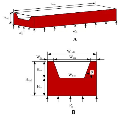
With the large ratio of length to hydraulic diameter, microchannel heat sinks are used to effectively remove higher heat fluxes from high power density electronic systems. Fig. 2 illustrates the geometry of a trapezoidal microchannel used to simulate flow instabilities of two-phase flow boiling. The geometry and dimensions of the microchannel correspond exactly to the experimental apparatus conducted by Wang et al. (2007). The width of top and bottom, and depth of the trapezoidal microchannel are 427 µm, 208 µm, and 146 µm, respectively. The angle at the base is 53 degree, the hydraulic diameter and length of the channel are 186 µm and 38 mm with inlet and outlet unheated region, respectively. The dimensions of the microchannel used in the computational simulation are given in Table 1. The thermal boundary condition on the bottom is the specified constant heat flux boundary condition and the adiabatic boundary conditions were assumed at the top and two side walls as shown in Fig. 2A. Based on Fig. 2B, wall heat flux,
q
w′′
is imposed on the microchannel heated inside area and is obtained as:
(
2eff cell/ sin)
w
bot ch
q W q
W H θ
′′ ′′ =
+ (1)
where qeff′′ is the imposed heat flux on the bottom of the microchannel,
cell
W and Wbot are the widths of the unit cell and microchannel,
respectively, Hchis the height of the heated trapezoidal microchannel.
θ
is the angle between the side surface and the horizontal surface of the microchannel.
A
B
Fig. 2Physical diagram of a trapezoidal microchannel. A) Schematic of a 3-D trapezoidal microchannel. B) Dimensions of the microchannel cross section.
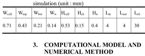
Fig. 3 shows the computational domain used in the three-dimensional numerical simulation for flow boiling. Taking advantage of symmetry condition, only half a channel is needed for the current numerical simulation as illustrated in Fig. 3A. Water is used as the working fluid with a constant and uniform inlet temperature, Tin, of 99.85 °C (373.0K), and it flows through the inlet plenum with an adiabatic condition. The subcooled liquid approaches up to the saturation temperature and vapor bubbles are generated on the heated wall. Two-phase mixture flows out of the outlet plenum with Tout and Pout as shown in Fig. 3B. The heat fluxes in the range of 297.8 – 495.4 kW/m2 are imposed on the heated inside wall and the mass fluxes of 679.5 – 3523.2 kg/m2∙s flow through the inlet region. The pressure outside of the outlet plenum is assumed to be the atmospheric pressure. Equally-spaced wall temperatures, Tw1, Tw2, Tw3, Tw4, and Tw5, were obtained on the heated wall along the flow direction as depicted in Fig. 3B.
Symmetry plane
′′ qw
′′ qw
y z
x Wtop/2
Wbot/2
A
B
Fig. 3Symmetric flow channel geometry used in the computational simulation. A). Half a microchannel. B) Flow region in the microchannel for the computational simulation.
Lch
Hcell
eff
q′′ qeff′′
θ Hch
Wtop Ww
Wbot
Hw
Wcell
eff q′′
Hcell
′′
qw
Lch
Lin Lout
, l in
T , l in
m Tpoutout
z y
1 w
T Tw2 Tw3 Tw4 Tw5
x L L2 L3 L4 L5
Table 1 Dimensions of a microchannel used in computational simulation (unit : mm)
Wcell Wtop Wbot Ww Hcell Hch Hw Lin Lout Lch
0.71 0.43 0.21 0.14 0.53 0.15 0.4 4 4 30
3.
COMPUTATIONAL MODEL AND
NUMERICAL METHOD
3.1 Governing Equations
Both liquid and vapor phases are assumed incompressible with variable thermal fluid properties. The gravitational effects are negligible because the surface effects are dominant in a microchannel. The continuity and momentum equations are
( )
V 0t
ρ ρ
∂ + ∇ • =
∂
(2)
( )
(
)
( )
sv
V
VV p V F
t ρ ρ µ ∂ + ∇ • = −∇ + ∇ • ∇ + ∂
(3)
The energy equation is
p E
T
c V T k T S
t
ρ ∂ + •∇ = ∇ • ∇ + ∂
(4)
The source terms sv
F and SE which denote interfacial mass, momentum, and energy interfacial exchange are included to simulate the two-phase flow boiling in a microchannel. The source terms will be discussed in the volume of fluid method below.
For the velocity boundary conditions, no-slip conditions are enforced on all the channel inside wall surfaces. A uniform and constant velocity,
in
u
, is specified at the inlet that is corresponding to the given constant mass flow rate,m
as follows :/ ( ), are water inlet density and inlet flow cross sectional area, respectively. At the outlet, atmospheric pressure is enforced.
in in in in in
u =m ρ A ρ and A
3.2 Numerical Method
3.2.1 Finite Volume Method
The ANSYS Fluent software package (Fluent, 2005) was employed to obtain the simulation results. Fluent uses the finite volume method (Patankar, 1980) to solve the governing equations associated with boundary and interfacial conditions. The details of the finite volume method and its implementation are skipped here as they have been considered a standard in computational fluid dynamics and heat transfer.
3.2.2 Volume of Fluid Method
The volume of fluid (VOF) model introduced by Hirt and Nichols (1981) was provided by Fluent (2005) for the modeling. The VOF technique solves a single set of momentum equations and determines the vapor-liquid interface shape of the two fluids by tracking the volume fraction
α
of each phase in each computational cell. The sum of the volume fraction of both phases is unity in each control volume. In this model, the vapor phase will be tracked and the volume fraction of the vapor phase isα
v. Each computational cell meets one of three conditions as follows: •α =
v0
: liquid phase only•
α =
v1
: vapor phase only• 0<
α
v<1: a two-phase mixture in the cellThe interface shape between both phases is tracked by solving the continuity equation for the volume fractions of phases. The continuity equation can be written as follows:
(
v v)
(
v vV)
St α ρ α ρ α
∂
+ ∇ ⋅ =
∂
(5)
where
α
v is the volume fraction for the vapor phase and Sα is the source term which represents the mass transfer accounting for phase change between the liquid and vapor phases. The volume fraction equation will not be solved for the primary phase. In the current model, the liquid phase is set to be the primary one; thus, the volume fraction of the primary phase,α
l, can be obtained from,1
l v
α = −α (6)
The discretized volume fraction equation with the first-order implicit scheme is obtained by using the finite volume approach as explained before:
(
)
(
)
(
)
1 1 n n nv v v v v v
faces
t V A S V
V α α ρ α ρ α ρ + + = + ∆ − ⋅ + ∆ ∆
∑
(7)
Based on the void fraction, a single momentum equation is solved for the entire computational domain and the resulting velocity field is shared among the phases as follows:
( ) (
V VV)
p(
V)
Fsvt ρ ρ µ
∂ + ∇ ⋅ = −∇ + ∇ ⋅ ∇ +
∂
(8)
where p is the pressure and Fsv is the surface tension force per unit volume, and
ρ
andµ
are the density and viscosity. Eq. (8) depends on the volume fractions of all phases through the properties ρ and µ. These properties are obtained by the presence of the computational phases in each control volume. The density and viscosity at the liquid-vapor interface vary with the volume fraction tracked as follows:(
1 v)
l v vρ= −α ρ α ρ+ (9)
(
1 v)
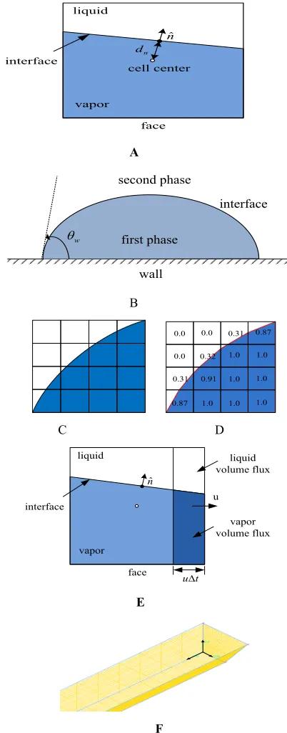
l v vµ= −α µ α µ+ (10) The source term in Eq. (8) is the surface tension force per unit volume and the gravitational forces are negligible in current study. The continuum surface force model of Brackbill et al. (1992) is used in Eq. (8). Fig. 4A shows a typical two-phase cell with an immersed phase interface. The surface curvature is defined in terms of the divergence of the unit normal vector as,
K= ∇ ⋅nˆ (11)
where K is the surface curvature and
n
ˆ
is the unit normal vector of the interface given by,ˆ s s
n n
n
= (12)
where
n
s is the surface normal vector defined as the gradient ofα
v as,ns= ∇αv (13)
Combining Eqs. (12) and (13) with Eq. (11), the curvature of the interface can be rewritten as,
v
v
K= ∇ ⋅∇∇αα
(14)
The source term in Eq. (8) can be expressed as a volume force as,
1 2
(
)
v sv
l v
K
F σ ρ α
ρ ρ ∇ =
+
(15)
where
ρ
is obtained from Eq. (9). For a three-phase contact line, thecontact angle θw is used to adjust the surface normal in cells near the wall. It results in the adjustment of the curvature of the surface near the wall. Thus, the unit normal vector at the cell near the wall is defined as
ˆ
ˆ ˆ cos
w w wsin
wwhere
n
ˆ
w andt
ˆ
ware the unit normal and tangential vectors to the wall,respectively, and θw defines the angle between the wall and the tangent
to the interface at the wall. The contact angle θw measures inside the first phase as shown in Fig. 4B. Eq. (16) with the normally calculated surface normal one cell away from the wall determines the local curvature of the surface.
To capture the liquid-vapor interface during the simulation, convection and diffusion fluxes through the control volume faces are calculated and balanced with source terms within the control volume in the finite volume method approach. Thus, in the VOF method, the interface is reconstructed at the beginning of a time step for more accurate simulation of its evolution as shown in Fig. 4C,D. When the cell is near the interface between two phases, the geometric reconstruction scheme is used. This scheme represents the interface between two phases using a piecewise-linear approach and uses this linear shape for calculation of the advection of fluid through the cell faces. The procedures of the scheme are as follows :
• The orientation of the curve within each two-phase cell is determined by Eq. (12) and Eq. (13).
• Given the orientation of the surface that represents the interface in a cell, determine the position
d
n of the linear interface relative to the center of each two-phase cell based on the volume fraction of the vapor as shown in Fig. 4A. These steps are often referred to as the interface reconstruction steps (Rider and Kothe, 1998).• The mass fluxes through each face are computed using the linear interface representation and information about the normal and tangential velocity distribution on the face as shown in Fig. 4E. Once the mass fluxes are calculated in one direction, the interface is reconstructed before the fluxes are determined in the other direction. • The volume fraction in each cell is determined by using the balance
of fluxes calculated during the previous step. The energy equation for the mixture is given by
( )
E V(
E p)
(
k T)
SEt ρ ρ
∂ + ∇ ⋅ + = ∇ ⋅ ∇ +
∂
(17)
where
S
E is the energy source term, that describes the latent heat transfer involved at the vapor-liquid interface during phase-change andk
is the thermal conductivity defined by,(
1 v)
l v vk= −
α
k +α
k (18)The VOF model treats energy and temperature as mass-averaged variables:
1
1 n
q q q
q n
q q
q
E E
α ρ
α ρ
=
=
=
∑
∑
(19)
where
E
q for each phase is based on the specific heat of that phase and the shared temperature. The liquid and vapor phase energies areand
l l v v
E h= E =h (20)
where h is the sensible enthalpy of the
q
th phase defined by,
ref
T
q T p q
h =
∫
c dT (21)The reference temperature used to calculate the enthalpy of each fluid is 298.15K in Eq. (21).
where Lt is the total length of a microchannel and Lp is the plenum length of inlet and outlet.
In current study, the ANSYS FLUENT software (Fluent, 2005) that is based on numerical methods detailed above is used to solve the
continuity, volume fraction equation, momentum and energy equations for the forced convective boiling in a microchannel.
A
w
θ first phase
interface
wall second phase
B
1.0 1.0 1.0
1.0 1.0 1.0
0.87 0.31 0.91
0.0 0.32 1.0 0.0 0.0 0.31 0.87
C D
E
F
Fig. 4 A. Two-phase cell with an embedded phase interface. B. Measuring the contact angle near the wall (FLUENT, 2005). C and D. Liquid-vapor interface calculation using volume fraction in each cell. C) Actual interface shape. D) Interface shape represented by the geometric reconstruction scheme using piecewise-linear interpolation. E. Calculation of volume flux through the face. F. Grid system of the three-dimensional CFD model.
The 3-D model geometry was created and meshed using the GAMBIT software provided by Fluent (2005). The grid system of half a flow channel was generated using hexahedral mesh elements for a 3-D
face vapor
liquid
interface
ˆ
n
cell center
n d
face vapor liquid
interface
ˆ
n
u t∆
u liquid volume flux
flow channel geometry as shown in Fig. 4F. The convergence of the mesh system was performed by decreasing the mesh sizes until the convergence criterion was met and the final grid density used in the current simulation is listed in Table 2.
Table 2 Grid density used in the computational simulation. Inlet plenum Flow channel Outlet plenum
20 20 40
×
×
20 20 500
×
×
20 20 80
×
×
3.2.3 Validation of Numerical Computation
We have tried to validate and verify our numerical computations extensively. The validity of the current numerical model and computational scheme is established by several close comparisons with experimental results on both the quantitative values and qualitative physical trends. Those comparisons are provided in Section 4 below.
Table 3 Simulation Conditions.
Case
q
eff′′
, kW/m2 G, kg/m2·sI 297.8 3523.2
II 307.6 711.8
III 495.4 679.5
4.
RESULTS AND DISCUSSION
Flow instabilities in a single trapezoidal microchannel have been investigated for three different cases as listed in Table 3 for various wall heat fluxes and working fluid mass fluxes. Case I (qeff′′ = 279.8 kW/m2 and G = 3523.2 kg/m2·s) represents low heat flux and high mass flux; Case II (qeff′′ = 307.6 kW/m2 and G = 711.8 kg/m2·s) is for medium heat flux and medium mass flux; and Case III (qeff′′ = 495.4 kW/m2 and
G = 679.5 kg/m2·s) stands for high heat flux and low mass flux.
4.1
Flow Boiling Patterns
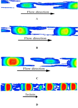
Flow boiling patterns predicted in the middle of the trapezoidal microchannel for Case I are shown in Fig. 5. When a liquid flow with a very small degree of subcooling enters a heated channel, nucleate boiling initiates very quickly downstream of the inlet as the heated channel wall temperature exceeds the amount of superheat required for boiling incipience. As the threshold of nucleate boiling strongly depends on the imposed heat flux and mass flux at a given inlet temperature and mass flux, vapor bubbles grow on the channel wall surface as nucleate boiling is initiated along the channel and then depart from the heated surface when the bubble size is large enough.
As more and more isolated single bubbles are entrained in the flow, the flow pattern becomes that of the bubbly flow at t = 12 ms as depicted in Fig. 5A. At t= 15 ms, the bubbles grow larger as they receive more heat from the surrounding superheated liquid that facilitates vaporization at the vapor bubble-liquid interface. As the bubbles grow larger, they coalesce with neighboring bubbles as shown in Fig. 5B. As a result, the flow pattern evolves from bubbly flow to slug flow. At t = 33.86 ms, similar to the vapor bubbles, the bubble slugs receive more heat from the superheated liquid and grow more along the channel direction such that the flow pattern becomes an elongated slug flow as shown in Fig. 5C. The flow patterns in the microchannel display a sequential and periodic
behavior : nucleate boiling, bubbly flow, bubbly/slug flow, and elongated slug flow as shown in Fig. 5D.
A
B
C
D
Fig. 5Flow patterns in the middle section of the trapezoidal microchannel for Case I. A) Bubbly flow at t = 12 ms, B) Transition from bubbly flow to slug flow at t = 15 ms, C) Elongated Slug flow at t = 33.86 ms, and D) Periodic flow boiling at t = 33.86 ms.
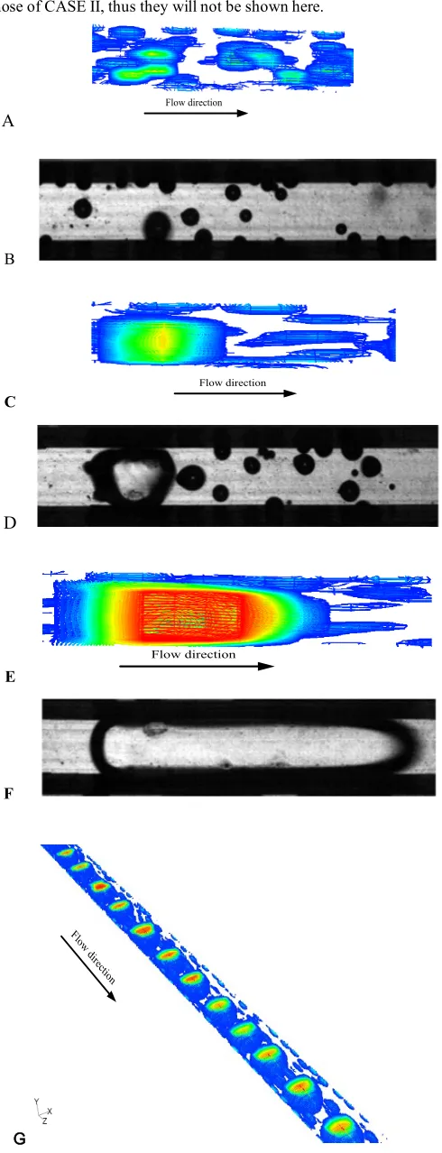
Fig. 6 shows flow boiling patterns predicted in the middle section of the microchannel for Case II. Generally, the flow patterns of Case II are similar to those of Case I for some portions of the flow. After boiling incipience, the flow pattern is also the isolated bubbly flow (at t = 5 ms) as shown in Fig. 6A. Bubbly flow transitions to bubbly-elongated bubble slug flow at t = 7 ms and then to elongated large bubble slug flow at t = 14.92 ms are provided in Fig. 6C and E. Periodic flow boiling pattern, also, is observed for Case II. The flow patterns of Case II obtained from the numerical simulation are consistent with the experimental observations by Wang et al. (2008) as demonstrated in Fig. 6. They observed isolated bubbles, bubble coalescence, and elongated bubbles as illustrated in Fig.s 6B, 6D and 6F. The transition from bubbly flow to slug bubble flow resulted from expansion and coalescence triggers flow instabilities in the microchannel. The elongated slug bubble prevents liquid mass from flowing through the flow channel. It causes the inlet pressure and wall temperature to increase and then oscillate. The increased inlet pressure forces the elongated slug bubble to move toward the channel exit. Small bubbles occur in the channel and the wall temperature decreases due to a rewetting process. It shows a periodic behavior as shown in Fig.s 5D and 6G. The flow instabilities potentially cause mechanical damage and operating control problem due to local dryout and periodic wall
Flow direction
Flow direction
Flow direction
temperature fluctuations. The flow patterns for CASE III are very similar to those of CASE II, thus they will not be shown here.
A
B
C
D
E
F
G
Fig. 6Flow patterns in the middle of the trapezoidal microchannel for
Case II. A) Isolated Bubbly flow at t = 5 ms, B) Isolated bubbly flow (Wang et al., 2008), C) Bubbly-elongated bubble slug transition flow at t = 7 ms, D) Bubbly-elongated bubble slug transition flow (Wang et al., 2008), E) Elongated large bubble slug flow at t = 14.92 ms, F) Elongated large bubble slug flow (Wang et al., 2008) and G) Periodic boiling at t = 14.92 ms.
4.2. Wall Temperature Fluctuations
With short-period oscillations, temporal variations of wall temperatures for Case I at lower heat flux and higher mass flux are depicted in Fig. 7. The wall temperature fluctuations are mainly initiated by the transition from bubbly to slug flow patterns. The temporal variations of wall temperature for Case I start at t = 15 ms when the transition begins (as shown in Fig. 7A). The results show that the amplitudes of wall temperature at Tw4 is much larger than those at Tw3. Tw3 displays a very small scale oscillations during the simulation period, while Tw4 shows higher oscillatory behavior. The reason is that the flow structure around Tw3 contains basically isolated bubbles (Fig. 6A) with a lower quality than that near Tw4 with slug flows as the large amplitude wall temperature oscillation is basically caused by wet (liquid) and dry (vapor) alternating conditions on a constant heat flux heater surface. Another important finding is that the temporal mean temperatures for both locations are relatively constant. Although the imposed heat flux, subcooling at the inlet, and channel geometry are moderately different, the obtained wall temperature fluctuations show qualitatively and quantitatively good agreement with the experimental results by Qu and Mudawar (2004) as shown in Fig. 7B. Their results also show that the wall temperature oscillations at Ttc4 have higher amplitudes than those at Ttc3. The quantitative discrepancy between the current results and the experimental data may be due to the relatively larger difference in inlet subcooling
levels. They used highly subcooled liquid (ΔTsub = 70 °C), while lower
subcooled liquid (ΔTsub = 1.5 °C) was used in this study. Higher subcooled liquid condenses some of the generated bubbles in the channel and before bubble departing and the bubble resides in the channel for a longer period, while lower subcooling leads to faster bubble departure and more coalescence. The trend of the obtained results also agrees with the experimental data by Xu et al. (2005). They pointed out that the periodic oscillations become shorter with increasing inlet temperature. Fig. 7C shows bubbly flow at t = 12 ms before starting oscillation (Region I in Fig. 7A). At t = 15 ms, bubbly to slug flow transition causes flow oscillation to start as illustrated in Fig. 7D (region II in Fig. 7A). Periodic boiling consisted of bubbly and elongated slug flows as depicted in Fig. 7D is dominant in region III in Fig. 7A. It leads to wall temperature fluctuations with a cyclic rewetting process.
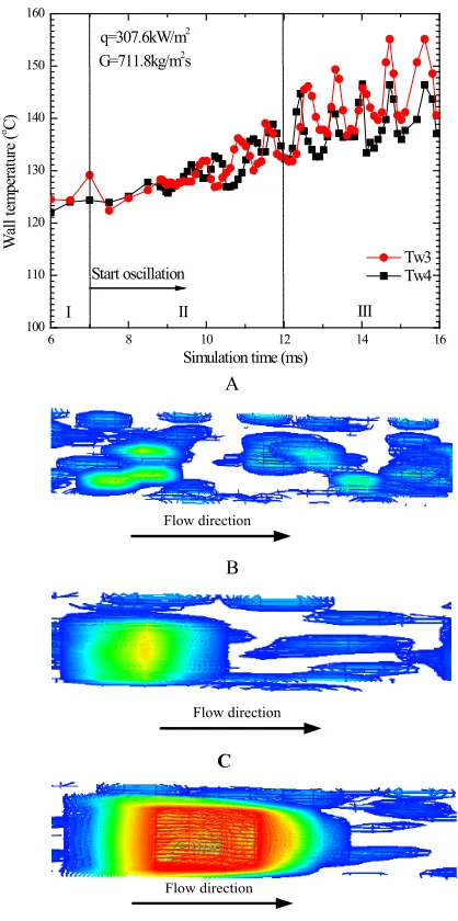
Temporal wall temperature fluctuations at Tw3 and Tw4 for Case II are shown in Fig. 8. Comparing to Case I, Case II has a similar wall heat flux level but the liquid inlet mass flux is only one fifth of that for Case I. As a result, the flow development and transition time are much quicker than Case I as shown in Figs. 5 and 6. In contrast with the results of Case I (as shown in Fig. 7A), the temporal wall temperature fluctuations at Tw3 are similar to those at Tw4. For both cases, the mean temperatures are rising with time.
The reason is that nucleate boiling is initiated near the inlet for Case II due to much smaller liquid inlet mass flux that also causes the bubbles to expand and coalesce near Tw3 rather than to be condensed. Wang et al. (2007) reported the same results as those in Case II. For the flow patterns, the bubbly flow is dominant in Region I as shown in Fig. 8B. At Region II, transition from bubbly flow to slug flow leads to increasing wall temperature fluctuations. Periodic flow boiling with elongated slug flow causes the higher wall temperature fluctuations in Region III as depicted in Fig. 8D. The peak-to-peak amplitude and oscillation period of wall temperature fluctuations are 15.44 °C and 1.6ms, respectively, as depicted in Fig. 8A.
Flow direction
Flow direction
Flow direction
A
B
C
D
E
Fig. 7 Wall temperature fluctuations with small amplitude and short-period oscillation, and flow patterns for Case I. A) Current result, B) Experimental investigation by Qu and Mudawar (2004), C) Bubbly flow at t = 12 ms (Region I), D) Bubbly-elongated transition at t = 15 ms (Region II), E) Elongated slug flow at t = 33.86 ms (Region III).
A
B
C
D
Fig. 8 Wall temperature fluctuations with large amplitude and short-period oscillation, and flow patterns for Case II. A) Wall temperature fluctuations, B) Isolated bubbly flow at t = 5 ms, C) Transition from bubbly flow to slug flow at t = 7 ms, and D) Elongated slug flow at t = 14.92 ms.
For Case III, the wall heat flux is 61% higher than that in Case II while the liquid mass flux at the inlet is about the same. Similar to Case II (as shown in Fig. 8A), the temporal wall temperature fluctuations at Tw3 are at the same levels to those at Tw4 as shown in Fig. 9. But the two are off-phase to each other due to wall heat flux difference. For both cases, again the mean temperatures are rising with time. Similarly with Case II, the wall temperature fluctuations are mainly affected by the periodic flow boiling pattern. The peak-to-peak amplitude and oscillation period of wall temperature fluctuations are 17.79 °C and 1.0 ms, respectively, as shown in Fig. 9. The amplitude and oscillation period of both Cases II and III show large amplitude and very short-period as a result of increasing heat flux and decreasing mass flux comparing to Case I. The current results are qualitatively consistent with the experimental investigation by Wang et al. (2007). In the current results, the amplitude of wall temperature fluctuations increases and the period of oscillation becomes shorter with increasing heat flux and decreasing mass flux. Wang et al. (2007) also showed that the wall temperatures at Tw3 and Tw4 increase as heat flux increases and mass flux decreases.
10 15 20 25 30 35 40 45 50
100 110 120 130 140 150 160
III II
II I
Wal
l tem
per
atu
re (
o C)
Simulation time (ms)
Tw3 Tw4 q=297.8kW/m2
G=3523.2kg/m2s
Start oscillation
t [s]
T
ci[
o
C
]
Flow direction
Flow direction
Flow direction
6 8 10 12 14 16
100 110 120 130 140 150 160
III II
W
all
tem
per
atu
re (
oC)
Simulation time (ms)
Tw3 Tw4 q=307.6kW/m2
G=711.8kg/m2s
Start oscillation
I
Flow direction
Flow direction
Fig. 9 Wall temperature fluctuations with large amplitude and short-period oscillation for Case III.
4.3. Pressure Fluctuations
Fig. 10 shows temporal variations of pressure fluctuations in the inlet and outlet regions for Case I. Pressure fluctuations at the channel inlet and outlet are induced by the alternating flow patterns between bubbly and elongated slug flow as shown in Fig.s 5B and 5C. The following provides the physics for the fluctuating nature of the inlet and outlet pressures. The transition between the bubbly and slug flows at t=15 ms (Fig. 5) leads to increasing inlet pressure as shown in Fig. 10A. The reason is that liquid mass flow is partially blocked by the elongated slug bubble in the flow channel after the bubbly/slug flow transition takes place and it leads to an instantaneous increase in the inlet pressure. In turn, the increased inlet pressure then pushes the elongated slug bubbles through the channel that causes the inlet pressure to decrease.
The outlet pressure fluctuations are lower in magnitude but still show a periodic behavior (Fig. 10B). The peak-to-peak amplitude and oscillation period of inlet pressure fluctuations is 6.5kPa and 1.9 ms, respectively. It is noted that for Case I, the period of inlet pressure fluctuations at 1.9 ms is very close to that of wall temperature oscillations at 1.8 ms as shown in Fig. 7A. The inlet and outlet pressure oscillations are also in phase as depicted in Fig. 10C. As compared with the experimental data of Qu and Mudawar (2003a) as shown in Fig. 10D, it is seen that qualitatively the simulated results have the same trends as those of the experimental data, while slightly different subcooling levels were used. The reason for the similar trends is that the flow patterns resemble each other in that they all started with a bubbly flow and then made a transition to elongated slug flow.
The temporal variations of the inlet pressure for Case II are illustrated in Fig. 11. The peak-to-peak amplitude and oscillation period of inlet pressure are 37.32 kPa and 1.1 ms, respectively (Fig. 11A). The results show that much higher pressure fluctuations than those of Case I are predicted as shown in Fig. 10A. The reason is again that the generation rate of vapor bubbles for Case II is five times greater than that for Case I due to the drastic reduction in the inlet liquid mass flux as listed in Table 3. Again, the currently predicted results are showing a similar trend with that of Wang et al. (2007) shown in Fig. 11B. As mentioned above, the oscillation period is shorter with increased inlet temperature. Thus, the oscillation period of the current study with higher inlet temperature is much shorter than that of Wang et al. (2007) with a lower inlet temperature. In addition, the difference between the current results and the experimental results may also be caused by the compressible volume near upstream and the annular/mist flow observed in their experiment.
A
B
C
D
Fig. 10 Inlet and outlet pressure fluctuations with small amplitude and short-period oscillation for Case I. A) Inlet pressure oscillations, B) Outlet pressure oscillation, C) Inlet and outlet pressure in phase and D)
6 7 8 9 10 11
120 130 140 150 160 170
W
al
l t
em
per
at
ur
e (
o C)
Simulation time (ms)
Tw3 Tw4 q=495.4kW/m2
G=697.5kg/m2s
Start oscillation 1.1515 20 25 30 35 40 45 50
1.20 1.25 1.30 1.35
G = 3523.2 kg/mq = 297.8 kW/m2s 2
Inl
et p
res
sure
(b
ar)
Simulation time (ms)
15 20 25 30 35 40 45 50
0.90 0.95 1.00 1.05 1.10 1.15 1.20
Out
let pr
ess
ure
(ba
r)
Simulation time (ms) G = 3523.2 kg/mq = 297.8 kW/m2s
2
46 47 48 49 50
0.9 1.0 1.1 1.2 1.3 1.4
pin
Pre
ssu
re (b
ar)
Simulation time (ms) pout
q = 297.8 kW/m2
G = 3523.2 kg/m2s
t (s)
P (
bar
A
B
Fig. 11 Inlet pressure fluctuations with large amplitude and short-period oscillation for Case II. A) Current result. B) Experimental data obtained by Wang et al. (2007).
Fig. 12 shows inlet pressure fluctuations for Case III. It is shown that the peak-to-peak amplitude and oscillation period of inlet pressure history are 76.70 kPa and 0.73 ms, respectively, as shown in Fig. 12A. The oscillation period reported by Wang et al. (2007) is 6.4 ms as illustrated in Fig. 12B. Both cases show that the amplitude and oscillation period of the inlet pressure are strongly affected by the increased wall heat flux. The amplitude of inlet pressure fluctuations is proportional to the imposed heat flux and the oscillation period of those is inversely proportional to the mass flux as listed in Table 4.
Table 4 Summary of the amplitude and oscillation of inlet pressure under different heat fluxes and mass fluxes.
Case qeff′′ ,
kW/m2 G,
kg/m2·s Amplitude (Peak-to-Peak), kPa Period, ms
I 297.8 3523.2 6.5 1.9
II 307.6 711.8 37.32 1.1
III 495.4 679.5 76.70 0.73
A
B
Fig. 12 Inlet pressure fluctuations with large amplitude and short-period oscillation for Case III. A) Current result. B) Experimental data obtained by Wang et al. (2007).
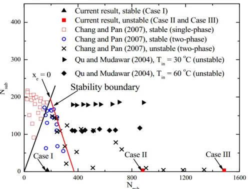
4.4. Stability Map
Fig. 13 shows the two-phase forced convective boiling stability map reported in Chang and Pan (2007) in terms of the subcooling number, Nsub, and the phase change number, Npch, as defined by,
i
sub
lv v
h N
h
ρ ρ
∆ ∆
= (22)
pch
lv v
Q N
mh
ρ ρ
∆ =
(23)
where
∆
h
i is the inlet subcooling,h
lvthe latent heat of vaporization,ρ
∆ the difference between liquid and vapor density,
ρ
v is the vapor density, Q the total heat input rate to the channels andm
the total mass flow rate to the channels. Chang and Pan (2007) constructed a stability map for a single microchannel based on the two-phase thermal instability theory developed by Saha et al. (1978) with experimental data from Qu and Mudawar (2004) in addition to their own results. The different sections on the map are divided by a solid line and a dotted line. The solid line represents that the exit vapor quality of the flow is equal to zero which means all the flows that fall to the left of this line are single-phase liquid flows. The dotted line denotes the stability boundary, so the triangular area bounded by the two lines is for stable two-phase flows6 8 10 12 14 16
1.00 1.25 1.50 1.75 2.00
In
le
t p
re
ss
ure
(b
ar)
Simulation time (ms) q=307.6kW/m2
G=711.8kg/m2s
Time (s)
Inlet pressure
(bar
)
5 6 7 8 9 10 11
1.00 1.25 1.50 1.75 2.00 2.25 2.50
In
let
pre
ssu
re (b
ar)
Simulation time (ms) q=495.4kW/m2
G=697.5kg/m2s
Time (s)
Inlet pressure
(bar
while the area to the right of the dotted line represents the unstable two-phase flows.
The three cases simulated in the current research are also placed in the map of Chang and Pan (2007). Case I is in the stable regime while Cases II and III are in the unstable regime. Since the subcooling numbers of the current cases are very small due to the low inlet subcooling, however the bulk of the experimental data from Chang and Pan (2007) and Qu and Mudawar (2004) have larger subcooling numbers due to the higher inlet subcooling. The phase change numbers of the current numerical results are higher because the phase change number is proportional to the imposed heat flux and inversely proportional to the mass flux. Table 5 lists the three cases and their stability outcomes.
It is important to point out that we believe that the stability map developed by Chang and Pan (2007) is applicable to the current simulated results based on the following analysis. As mentioned in Section 4.2 on wall temperature fluctuations, the mean temperatures for both Tw3 and Tw4 locations are relatively constant (Fig. 7A) for Case I while they are on a rising trend for both Cases II and III (Fig. 8A and Fig. 9). Based on the wall temperature fluctuation patterns, Case I is considered stable and Cases II and III are unstable.
Fig. 13 Stability map in subcooling number versus phase change number based on Chang and Pan (2007).
5.
CONCLUSION
A 3-D numerical model was used to simulate the convective boiling heat transfer in a trapezoidal microchannel. The heated wall temperature and flow inlet pressure oscillations characterizing the flow instabilities are
investigated in a microchannel with a hydraulic diameter of 186 μm.
Results were obtained for various wall heat flux levels, inlet flow subcooling values and mass flow rates. The simulated flow patterns in the microchannel display a sequential and periodic phenomenon that includes nucleate boiling incipience, bubbly flow, slug flow, and elongated slug flow. The wall temperature fluctuations are mainly initiated by the transition from bubbly to slug flow patterns. It is found that with increasing wall heat flux and decreasing mass flux, the amplitude of wall temperature fluctuations increases and the period of oscillation becomes shorter. The obtained numerical results on wall temperature fluctuations show close qualitative and quantitative agreement with the experimental results by Qu and Mudawar (2004). Pressure fluctuations at the channel inlet and outlet were shown to be induced by the alternating flow patterns between bubbly and elongated slug flow. It was also noted that the amplitude and oscillation period of the inlet pressure fluctuations are strongly affected by the increased wall heat flux. The amplitude of inlet pressure fluctuations is
proportional to the imposed heat flux and the oscillation period of those is inversely proportional to the mass flux.
The current study focused on the low subcooling number condition with a wide range of the phase change numbers. Based on the simulated results, stable and unstable cases were identified by the different phase change numbers as the three cases invested all fit correctly in the flow boiling stability map developed by Chang and Pan (2007).
Table 5 Summary of stable and unstable flow boiling regime under different heat fluxes and mass fluxes.
Case I II III
eff
q
′′
, kW/m2 297.8 307.6 495.4G, kg/m2·s 3523.2 711.8 679.5
eff
q G′′ , kJ/kg 0.08 0.43 0.73
Remark
Stable with small amplitude and short period
Unstable with large amplitude and short period
Unstable with large amplitude and short period
ACKNOWLEDGEMENTS
The research was support by the Andrew H. Hines, Jr./Progress Energy Endowment Fund.
NOMENCLATURE
A surface vector [m2] Cp specific heat [J/kg·K] f frequency [Hz] G mass flux [kg/m2·s] H channel height [mm]
hlv latent heat of vaporization [J/kg] hc heat transfer coefficient [W/m2·K]
hsp ingle phase heat transfer coefficient [W/m2K] k thermal conductivity [W/m·K]
m
mass flow rate [kg/s]m′′ mass flux [kg/m2·s] Npch phase change number Nsub subcooling number p pressure [Pa]
q′′ heat flux [W/m2] T temperature [K] t time [s]
u mean velocity [m/s] V velocity vector [m/s]
V control volume in the finite volume scheme W channel width [mm]
x x coordinate y y coordinate z z coordinate
Greek Symbols
α volume fraction, thermal diffusivity [m2/s]
Δ variable difference
μ dynamic viscosity [kg/m·s2]
ν kinematic viscosity [m2/s]
Subscripts
eff effective heat flux imposed on microchannel heat sinks in channel inlet
h hydraulic
l
liquidONB onset of nucleate boiling out channel outlet
q phase q sub subcooling v vapor phase
w wall of a heated flow channel; Width; Waiting time z axial direction
REFERENCES
Bergles, A.E., 1981, “Instabilities in Two-Phase Systems,” Two-Phase Flow and Heat Transfer in the Power and Process Industries, Hemisphere, Washington, DC, 383-411.
Boure, J.A., Bergles, A.E., and Tong, L.S., 1973, “Review of Two-Phase Flow Instability,” Nucl. Eng. Des., 25, 165-192.
https://doi.org/10.1016/0029-5493(73)90043-5
Bowers, M.B., and Mudawar, I., 1994a, “High Flux Boiling in Low Flow Rate, Low Pressure Drop Mini-Channel and Micro-Channel Heat Sinks,” Int. J. Heat Mass Transfer, 37, 321-332.
https://doi.org/10.1016/0017-9310(94)90103-1
Brackbill, J.U., Kothe, D.B. and Zemach, C., 1992, “A Continuum Method for Modeling Surface Tension,” J. Comput. Phys., 100, 335-354.
https://doi.org/10.1016/0021-9991(92)90240-Y
Brutin, D., and Tadrist, L., 2004, “Pressure Drop and Heat Transfer Analysis of Flow boiling in a Minichannel: Influence of the Inlet Condition on Two-Phase Flow Stability,” Int. J. Heat Mass Transfer, 47, 2365-2377.
https://doi.org/10.1016/j.ijheatmasstransfer.2003.11.007
Brutin, D., Topin, F., and Tadrist, L., 2003, “Experimental Study of Unsteady Convective Boiling in Heated Minichannels,” Int. J. Heat Mass Transfer, 46, 2957-2965.
https://doi.org/10.1016/S0017-9310(03)00093-0
Chang, K. H., and Pan, C., 2007, “Two-Phase Flow Instability for Boiling in a Microchannel Heat Sink,” Int. J. Heat Mass Transfer, 50,
2078-2088.
https://doi.org/10.1016/j.ijheatmasstransfer.2006.11.014
Cheng, P., and Wu, H.Y., 2006, “Mesoscale and Microscale Phase-Change Heat Transfer,” Adv. in Heat Transfer, 39, 461-563.
https://doi.org/10.1016/S0065-2717(06)39005-3
Coleman, J.W., and Garimella, S., 1999, “Characterization of Two-Phase Flow Patterns in Small Diameter Round and Rectangular Tubes,” Int. J. Heat Mass Transfer, 42, 2869-2881.
https://doi.org/10.1016/S0017-9310(98)00362-7
FLUENT 6.2 Users Guide, 2005, Fluent Inc., Lebanon, New Hampshire.
Ghiaasiaan, S.M., 2008, Two-Phase Flow, Boiling, and Condensation in Conventional and Miniature Systems, Cambridge University Press, New York, NY.
Hetsroni, G., Mosyak, A., Pogrebnyak, E., and Segal, Z., 2005, “Explosive Boiling of Water in Parallel Micro-Channels,” Int. J. Multiphase Flow, 31, 371-392.
https://doi.org/10.1016/j.ijmultiphaseflow.2005.01.003
Hetsroni, G., Mosyak, A., Segal, Z., and Ziskind, G., 2002, “A Uniform Temperature Heat Sink for Cooling of Electronic Devices,” Int. J. Heat Mass Transfer, 45, 3275-3286.
https://doi.org/10.1016/S0017-9310(02)00048-0
Hirt, C. W. and Nichols, B. D., 1981, “Volume of Fluid (VOF) Method for the Dynamics of Free Boundary,” J. Comput. Phys., 39, 201-225.
https://doi.org/10.1016/0021-9991(81)90145-5
Huh, C., Kim, J., and Kim, M. H., 2007, “Flow Pattern Transition Instability during Flow boiling in a Single Microchannel,” Int. J. Heat Mass Transfer, 50, 1049-1060.
https://doi.org/10.1016/j.ijheatmasstransfer.2006.07.027
Kakac, S., and Bon, B., 2008, “A Review of Two-Phase Flow Dynamic Instabilities in Tube Boiling Systems,” Int. J. Heat Mass Transfer, 51, 399-433.
https://doi.org/10.1016/j.ijheatmasstransfer.2007.09.026
Kakac, S., Veziroglu, T.N., Ozboya, N., and Lee, S.S., 1990, “Investigation of Thermal Instabilities in a Forced Convective Upward Boiling System,” Exp. Therm. Fluid Sci., 3, 191-201.
https://doi.org/10.1016/0894-1777(90)90087-N
Kandlikar, S. G., Steinke, M. E., Tian, S., Campbell, L. A., 2001, “High- Speed Photographic Observation of Flow Boiling of Water in Parallel Minichannels,” Proceedings of National Heat Transfer Conference, ASME, Anaheim, CA, 765-684.
Kosar, A., Kuo, C. J., and Peles, Y., 2005, “Suppression of Boiling Flow Oscillations in Parallel Microchannels by Inlet Restrictors,” J. Heat Transfer, 128, 251-260.
https://doi.org/10.1115/1.2150837
Kuo, C. J., Kosar, A., Peles, Y., Virost, S., Mishra, C., and Jensen, M. K., 2006, “Bubble Dynamics During Boiling in Enhanced Surface Microchannels,” J. Microelectromech. Syst., 15, 1514-1527.
https://doi.org/10.1109/JMEMS.2006.885975
Ledinegg, M., 1938, Instability of flow during natural and forced circulation, Die Waerme, 61, 891-898.
Muwanga, R., Hassan, I., and MacDonald, R., 2007, “Characteristics of Flow Boiling Oscillations in Silicon Microchannel Heat Sinks,” J. Heat Transfer., 129, 1341-1351.
https://doi.org/10.1115/1.2754946
Nayak, A. K., Vijayan, P. K., Jain, V., Saha, D., and Sinha, R. K., 2003, “Study on the Flow-Pattern-Transition Instability in a Natural Circulation Heavy Water Moderated Boiling Light Water Cooled Reactor,” Nucl. Eng. Des., 225, 159-172.
https://doi.org/10.1016/S0029-5493(03)00153-5
Patankar, S.V., 1980. Numerical Heat Transfer and Fluid Flow, Hemisphere Publishing Company, Washington, DC.
Qu, W., and Mudawar, I., 2003a, “Measurement and Prediction of Pressure Drop in Two-Phase Microchannel Heat sinks,” Int. J. Heat Mass Transfer, 46, 2737-2753.