SIMULATION AND OPTIMIZATION OF A CROSSDOCKING OPERATION IN A JUST-IN-TIME ENVIRONMENT

(1)

University of Kentucky University of Kentucky

UKnowledge

University of Kentucky Doctoral Dissertations Graduate School

2002

SIMULATION AND OPTIMIZATION OF A CROSSDOCKING

OPERATION IN A JUST-IN-TIME ENVIRONMENT

Karina Hauser

University of Kentucky, [email protected]

Right click to open a feedback form in a new tab to let us know how this document benefits you. Right click to open a feedback form in a new tab to let us know how this document benefits you.

Recommended Citation Recommended Citation

Hauser, Karina, "SIMULATION AND OPTIMIZATION OF A CROSSDOCKING OPERATION IN A JUST-IN-TIME ENVIRONMENT" (2002). University of Kentucky Doctoral Dissertations. 275.

https://uknowledge.uky.edu/gradschool_diss/275

(2)

ABSTRACT OF DISSERTATION

Karina Hauser

The Graduate School University of Kentucky

(3)

SIMULATION AND OPTIMIZATION OF A CROSSDOCKING OPERATION IN A JUST-IN-TIME ENVIRONMENT

Abstract of Dissertation

A dissertation submitted in partial fulfillment

of the requirements for the degree of Doctor of Philosophy in the College of Business and Economics

at the University of Kentucky By

Karina Hauser Lexington, Kentucky

Director: Dr. Chen Hua Chung, Gatton Endowed Professor of DSIS University of Kentucky

Lexington, Kentucky 2002

(4)

ABSTRACT OF DISSERTATION

SIMULATION AND OPTIMIZATION OF A CROSSDOCKING OPERATION IN A JUST-IN-TIME ENVIRONMENT

In an ideal Just-in-Time (JIT) production environment, parts should be delivered to the work-stations at the exact time they are needed and in the exact quantity required. In reality, for most components/subassemblies this is neither practical nor economical. In this study, the material flow of the crossdocking operation at the Toyota Motor Manufacturing plant in Georgetown, KY (TMMK) is simulated and analyzed.

At the Georgetown plant between 80 and 120 trucks are unloaded every day, with approxi-mately 1300 different parts being handled in the crossdocking area. The crossdocking area consists of 12 lanes, each lane corresponding to one section of the assembly line. Whereas some pallets contain parts designated for only one lane, other parts are delivered in such small quantities that they arrive as mixed pallets. These pallets have to be sorted/crossdocked into the proper lanes before they can be delivered to the workstations at the assembly line. This procedure is both time consuming and costly.

In this study, the present layout of the crossdocking area at Toyota and a layout proposed by Toyota are compared via simulation with three newly designed layouts. The simulation mod-els will test the influence of two different volumes of incoming quantities, the actual volume as it is now and one of 50% reduced volume. The models will also examine the effects of crossdocking on the performance of the system, simulating three different percentage levels of pallets that have to be crossdocked.

(5)

project, the design will be further optimized. Starting with the best layouts from the simu-lation results, the lanes will be rearranged using a genetic algorithm to allow the lanes with the most crossdocking traffic to be closest together.

The different crossdocking quantities and percentages of crossdocking pallets in the simu-lations allow a generalization of the study and the development of guidelines for layouts of other types of crossdocking operations. The simulation and optimization can be used as a basis for further studies of material flow in JIT and/or crossdocking environments.

KEYWORDS: Crossdocking, Simulation, Optimization, Genetic Algorithms

(6)

By Karina Hauser

Dr. Chen Hua Chung Director of Dissertation

Dr. Michael Tearney Director of Graduate Studies

(7)

RULES FOR THE USE OF DISSERTATIONS

Unpublished dissertations submitted for the Doctor’s degree and deposited in the Unversity of Kentucky Library are as a rule open for inspections, but are to be used only with due regard to the rights of the authors. Bibliographical references may be noted, but quotations or summaries of parts may be published only with the permission of the author, and with the ususal scholarly acknowledgments.

(8)

DISSERTATION

Karina Hauser

The Graduate School University of Kentucky

(9)

Dissertation

A dissertation submitted in partial fulfillment

of the requirements for the degree of Doctor of Philosophy in the College of Business and Economics

at the University of Kentucky By

Karina Hauser Lexington, Kentucky

Director: Dr. Chen Hua Chung, Gatton Endowed Professor of DSIS University of Kentucky

Lexington, Kentucky 2002

(10)

Acknowledgements

(11)

List of Figures

1.1 Layout of the unloading/lane storage/assembly line area . . . 3

1.2 Flow kanban cards . . . 4

1.3 Lane layout . . . 5

2.1 A typical layout produced by the models of Bartholdi and Gue . . . 12

3.1 New layout 1 . . . 20

3.2 New layout 2 . . . 21

3.3 New layout 3 . . . 21

3.4 New layout proposed by Toyota . . . 23

3.5 Algorithm to build pallets . . . 25

3.6 Main model . . . 28

3.7 Submodel: Unwrapping . . . 29

3.8 Submodel: Next Unwrap . . . 29

3.9 Submodel: Transfer . . . 30

3.10 Submodel: Next Transfer . . . 30

3.11 Model: Which lane to unwrap first . . . 31

3.12 Model: End of simulation . . . 32

3.13 Number of boxes per 20 minute interval for current data . . . 33

3.14 Number of boxes per lane for current data . . . 34

(16)

3.16 Number of boxes per lane for data from Toyota’s proposed changes . . . . 38

3.17 Comparison of differences in number of boxes per lane using current data and data from Toyota’s proposed changes . . . 39

3.18 Crossdocking area original layout with measurements . . . 41

3.19 Crossdocking area of new layout 1, with measurements . . . 43

3.22 Crossdocking area of layout proposed by Toyota with measurements . . . . 48

(17)

List of Tables

2.1 Genetic Algorithm parameters part 1 . . . 16

3.1 Possible combinations of the three simulation parameters . . . 24

3.2 Number of boxes per 20 minute interval for current data . . . 32

3.3 Cumulative data per lane for current data . . . 33

3.4 Flowmatrix for current data . . . 35

3.5 Number of boxes per 20 minute interval for data from Toyota’s proposed changes . . . 35

3.6 Cumulative data boxes per lane for data from Toyota’s proposed changes . . 37

3.7 Flowmatrix for data from Toyota’s proposed changes . . . 37

3.8 Travel distances original layout . . . 42

3.9 Travel distances new layout 1 . . . 44

3.12 Travel distances for layout proposed by Toyota . . . 49

4.1 Crossdocking activity between lanes in percentages for current data . . . . 51

4.2 ANOVA total distance for current data . . . 52

(18)

4.5 T-test results: Original layout vs. new layout 3 for current data . . . 54

4.6 Comparison of walking distance for current data . . . 55

4.7 Comparison of dolly distance for current data . . . 55

4.8 Improvements of layouts by speed of dollies . . . 56

4.9 Crossdocking activity between lanes in percentages for data from Toyota’s proposed changes . . . 57

4.10 ANOVA total distance for data from Toyota’s proposed changes . . . 58

4.11 Individual t-tests for data from Toyota’s proposed changes . . . 58

4.12 ANOVA total distance = walking distance + dolly distance/3 for data from Toyota’s proposed changes . . . 59

4.13 T-test results: Toyota’s proposed new layout vs. new layout 3 . . . 59

4.14 Comparison of walking distance for data from Toyota’s proposed changes . 60 4.15 Comparison of dolly distances for data from Toyota’s proposed changes . . 60

4.16 Comparison of improvement percentages control layouts vs. new layouts . . 60

4.17 Examples of different Quantities and Crossdocking % . . . 63

5.1 Start population for example . . . 67

5.2 Example pallet . . . 68

5.3 Distances between unloading point and the lanes . . . 68

5.4 Results of GA parameter selection experiments . . . 72

5.5 Connection Table and selection of genes to create offspring . . . 73

5.6 Optimized layouts . . . 75

6.1 Overview improvements for current data . . . 76

6.2 Results analysis for current data . . . 78

6.3 Overview improvements for data from Toyota’s proposed changes . . . 78

(19)

List of Files

(20)

Chapter 1 Introduction

The pressure to produce a wide variety of models has made mixed-model assembly lines an integral part of the Just-in-Time (JIT) production system. On a mixed-model assembly line, several different models of a basic end product are produced at the same time, for example, Camrys with and without moon-roof, with right or left steering. This leads to the problem of balancing and sequencing the different models on the assembly line. One of the goals of sequencing is to keep the usage of every part in the assembly line constant to ensure a smooth production. Many algorithms have been developed to help with the sequencing of mixed-model assembly lines, but little attention has been paid to the challenges that frequent deliveries pose for the support people in the logistics area. The goal to keep inventory low leads to frequent deliveries and the need for innovative storage and transportation solutions. In an ideal situation, the suppliers would deliver the needed parts directly to the workstation at the assembly line in the exact quantity at the exact time and in the sequence needed. In this ideal case, the inventory level at and between all workstations would be zero. In reality, only a few parts are delivered directly in sequence to the assembly line, for example, car seats, thus different intermediate storage solutions have been developed:

(21)

Internal Sequencing: If parts are needed in a special sequence at the line, they are stored in a sequence area and sequenced before delivery to the line.

Lane storage: Here the incoming parts are sorted by line and then are immediately delivered to the line. This sorting process is called crossdocking. Traditionally, crossdocking is defined as “a logistic technique that eliminates the storage and order picking functions of a warehouse while still allowing it to serve its receiving and shipping functions” [Bartholdi III and Gue, 2001] and it is used in the less-than-truckload freight industry. In this study, the shipping function is replaced by the consumption of the parts at the assembly line.

1.1 Statement of the Problem

The project will be performed in cooperation with Toyota Motor Manufacturing Kentucky (TMMK). Personnel planning in the lane storage area poses a problem for TMMKs inter-nal logistic manager. Team members complain about the unbalanced workload; some team members are unable to handle their workload, whereas others have too little work. In addi-tion, this workload imbalance varies during a typical work day. Team members support each other, but they would prefer a solution equalizing workloads overall and during the whole day. An evenly distributed workload not only establishes a sense of equity among workers but, more importantly, increases the output.

The part requirement schedule and the delivery schedule of the incoming parts are the two factors that directly influence the workload balance in the crossdocking area. Studying the influence of these two factors is beyond the scope of this dissertation. The other factor that influences the workload balance is the workload itself. By reducing the overall workload, the remaining workload is easier to balance; so this study concentrates on minimizing the workload in the crossdocking area.

The logistics manager also would appreciate a tool to better understand the factors leading to this imbalance. For example, how changes in the volume of incoming parts, influence the behavior of the material flow in the logistics area.

1.2 Description of the Lane Storage Area at Toyota

(22)

the team members in that area. The trucks have retractable sides which allow unloading from both sides simultaneously. Two forklift drivers, dedicated to unloading, are able to unload the whole truck within 5 minutes.

Between 20 and 30 trucks per pit are unloaded every day, which totals between 80 and 120 trucks per day. The truck schedule generally remains constant, although some trucks do not come in on a daily basis. Once a month the sequence schedule for the assembly line changes, and the truck schedule changes accordingly. These schedule changes also take into account the mileage per carrier and attempt to equalize it. In addition to the parts that are handled in the lane storage area, the trucks carry parts for other storage areas, such as sequencing parts and flowrack parts.

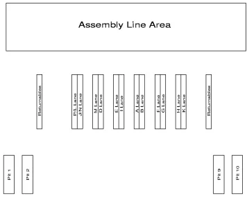
Figure 1.1: Layout of the unloading/lane storage/assembly line area

(23)

lineside/lane addresses. Therefore, in this study, parts with multiple uses and destinations can be considered as different parts. The flow of the kanban cards is shown in Figure 1.2.

Each part has a cycle time Cycle time information: - daily/weekly - deliveries per day - number of trucks between the same kanban card (delay time) example: cycle time 11015 1 = daily

10 = 10 times per day 15 = if a certain kanban card goes to the supplier it comes back in on the 15th truck from that supplier

Information on Kanban card: - Part Number - Part Description - Supplier - Qty/Container - Lane Storage Address - Kanban No Kanban Card

created Supplier receives

Kanban Card

Parts come in with Kanban Card

Parts/Kanban brought into lane

storage area

Parts/Kanban brought to assembly

line

Kanban pulled if 1st part in container is

used Kanban Cards

collected Kanban sorted by

supplier Kanban sent to

supplier

Figure 1.2: Flow kanban cards

The number of team members is currently fixed at 8 working in the delivery area and 3 team members working in the sorting area. Every two hours, team members in the lane storage area rotate between crossdocking and delivery to line. Forklift drivers rotate jobs on a daily basis.

The lane storage area consists of 14 lanes, with two sets of lanes (P/L and J/N, as shown in Figure 1.1) sharing the same physical space; thus for this study they are considered one lane, so overall there are 12 lanes. The lanes and lines have corresponding labels, e.g., all dollies/parts from lane E go to a part of the assembly line that is also labeled E. For the remainder of this study, the lanes are labeled according to their position in the layout, e.g., lane P/L will be labeled lane 1, lane J/N will be labeled lane 2, etc. Each lane is separated into 3 sections, as shown in Figure 1.3.

• Lane Section 1: Unloading area 5 dollies

(24)

• Lane Section 2: Crossdocking area 5 dollies

The crossdocking area is separated from the waiting area by a red line; only electric cars, called tuggers, operate behind the red line, no forklifts are allowed. A team member pulls all full dollies from the loading area into the crossdocking area, removes the packaging material and sorts out parts (crossdocking) that do not belong to that lane. If the lane is close by, the team members bring the boxes there directly; if not, the parts are stored on a dolly that stands between the lanes. When the team member has time, the mixed dolly is unloaded at the proper lanes .

• Lane Section 3: Line delivery area 5 dollies

After crossdocking, the team member pulls the dollies into the ready area where they wait until a team member from the delivery team is able to bring them to the assembly line.

Line

Loading Area Crossdocking Area Unloading Area

Figure 1.3: Lane layout

At the line, the parts are unloaded into a designated row in a flowrack. If the flowrack is full, the parts go into the overflow area for that workstation.

1.3 Research Goals and Contribution

(25)

transportation are viewed as non-value adding elements of a manufacturing operation, they have to be kept to a minimum.

De Haan and Yamamoto [de Haan and Yamamoto, 1999] showed in their case study that zero inventory is, for the moment, more fiction than fact. In a study of inventory methods of eight Japanese companies’, seven out of the eight companies inventory methods for raw material, depended on the distance between the supplier and the buyer. Suppliers that are located in close proximity to the buyers’ plant deliver daily, whereas the other suppliers have a weekly or even monthly delivery interval. Of the eight surveyed companies, only one, a make-to-order company, found the goal of zero inventory more disruptive to their production process than helpful and had its material delivered on a weekly basis.

The research in this study acknowledges that zero inventory is in reality not possible and that solutions have to be found to handle the incoming material efficiently. The overall goal of this research to identify the factors that can lead to an improvement in the workload of the team members in the crossdocking operation. This will be done through analyzing and optimizing the material flow from the unloading of the material from trucks to the unloading of the material at the workstations where it is used.

The first objective of the simulation is the analysis of the material flow and the identification of all parameters that are involved. After identification of the parameters, the influence of these parameters on the workload of the team members is analyzed. This will lead to a better understanding of the whole system and the identification of potential bottlenecks and problems.

The objective of the optimization is to rearrange the lanes, so that lanes that have the most crossdocking activity are closest together, and that the workload balance among the team members can be further improved. The workload balance is directly influenced by the sched-ule of part requirements (i.e. production schedsched-ule) and the delivery schedsched-ule of the incoming material resulting from it. Studying the influence of these parameters is beyond the scope of this dissertation. This work concentrates on minimizing the overall workload for the team members in the crossdocking area. An overall lower workload will simplify the task of workload balancing.

Therefore the overall objective is to reduce the traveling distance of the team members in the crossdocking area. The reduced traveling distance will lead to lower handling cost as well as decreased lead time between unloading of the truck and unloading of the parts at the assembly line. The reduced lead time has two effects: first, it will reduce the workload of the team members, and second, it will reduce the inventory level of raw material.

(26)

(27)

Chapter 2 Literature Review

This chapter starts with a review of the existing JIT literature related to the delivery/logistics process of the supply chain management, followed by a brief overview of mixed-model as-sembly line literature, which covers the front end and the back end of the crossdocking operation. Then the existing crossdocking literature is summarized, and finally, an exami-nation of facility layout studies, especially those using the Quadratic Assignment Problem approach, is made.

2.1 Review of JIT Delivery Literature

In JIT delivery, the materials are provided to the production plant just as they are required for use. JIT delivery is part of the larger concept of JIT purchasing, which includes a small, reliable supplier base close to the buyer’s plant and frequent deliveries. Schonberger [Schonberger, 1984] describes a smooth flow of materials between suppliers and buyers as one of the key elements needed to ensure a continuous process from receipt of raw mate-rial/components through to the shipment of the finished goods.

(28)

Hale [Hale, 1999] points out some of the challenges and opportunities awaiting logistics in the new millennium. With more people shopping via the Internet and home shopping channels, he expects a substantial increase in home deliveries. These small order deliveries present new logistical challenges for all partners, including more non-stop logistic move-ment, such as:

1. crossdocking

2. consolidation of products from multiple manufacturers by third-party logistics providers in a single delivery

3. increased emphasis on point-of- sale driven, pull inventory replenishment systems 4. increased demand for customized deliveries of multi-tier pallets with electronic pallet

content identification

5. advanced electronic data interchange (EDI) capabilities

Real time information flow will be an essential component in the logistic chain. These chal-lenges can only be handled by providing logistics managers with new tools such as: high speed networks, satellites for location of transportation vehicles, easier to use activity-based costing systems, and user friendly modeling, simulation and optimization techniques that support managers in their decision.

Fisher [Fisher, 1997] found that the logistic approach should depend on the type of products. He distinguished two different product types: functional products, which are characterized by a predictable demand, a high forecast accuracy, low stockout rate and low product variety, and innovative products, which are characterized by an unpredictable demand, low forecast accuracy, high stockout rate and high product variety. To handle functional products, he suggests concentrating on minimizing the physical costs that appear in the supply chain, such as cost of transportation and handling. To handle innovative products, he suggests concentrating on the market mediation costs, which occur when the supply is greater than the demand and force prices to drop, or when demand exceeds supply, resulting in lost sales opportunities and dissatisfied customers.

2.2 Review of Mixed-Model Assembly Line Literature

(29)

they also present two challenges. The first challenge is the design and balancing of the assembly line, which includes determination of cycle times and number of workstations. The second challenge is the sequencing of the different models on the assembly line, which can be divided into smoothing and leveling. In smoothing, the goal is to assign each workstation in the assembly line an equal amount of work so that the operation time is the same at all workstations. The goal of leveling is to sequence the models so that all subassemblies and components are withdrawn equally and so that the overall variability is minimized, which at the end leads to a minimized overall inventory. Sequencing mixed-model assembly lines has gotten a lot of attention in the literature.

Leu et al. [Leu et al., 1996] give an excellent illustration of the difficulties faced while se-quencing a mixed-model assembly line. They developed a genetic algorithm that improves upon Toyota’s Goal Chasing Algorithm and gets results within seconds. The algorithm was tested on 80 problems with the result of improved sequence in 50 of the problems. Using Toyota’s variability of part consumption criterion, the algorithm achieved a performance ad-vantage of 2% across all 80 problems. Korkmazel and Meral [Korkmazel and Meral, 2001] first compare the performance of some well-known approaches [Inman and Buffin, 1991] [Miltenburg, 1989][Ding and Cheng, 1993a][Ding and Cheng, 1993b] for solving the level-ing problem to the optimal solution obtained by uslevel-ing the shortest path algorithm of Burkard and Derigs [Burkard and Derigs, 1980]. The approaches found to be performing better are extended to incorporate the goal of smoothing the workload. In addition, the conditions under which it is important to take the workload-smoothing goal into consideration are an-alyzed. They found that high variance in model processing and/or shorter lines makes con-sidering the workload-smoothing goal worthwhile.

Matanachai and Yano [Matanachai and Yano, 2001] propose a new line balancing approach with the emphasis on providing a stable workload on the assembly line while also achieving reasonable workload balance among all workstations. They first compare their heuristic fil-tered beam search algorithm with a commercial mixed-integer optimizer for a small problem and report improvements of 22% to 41%, depending on the average utilization of the line and the variability of the task processing time. They then used their approach on a set of larger problems and also found substantial improvements in 90% of the problems.

(30)

improvements occur after that. Increasing the number of kanbans also results in an increase in waiting times and WIP length. On the contrary, an increase in the coefficient of variation of processing time or degree of imbalance leads to a decrease in output rate and utilization.

2.3 Review of Crossdocking Literature

The success story of Wal-Mart [Stalk et al., 1992] and its improvement in lead time has brought attention to crossdocking operations. Wal-Mart achieved its goal of providing cus-tomers access to quality goods when and where they want them by making the way the company replenished inventory the centerpiece of its competitive strategy. Due to cross-docking, goods cross from one loading dock to another within 48 hours or less. By running 85% of its goods through its warehouse system, Wal-Mart reduced costs of sales by 2% to 3% compared to the industry average.

Gue [Gue, 1999] defines terminal layout as the arrangement of receiving/strip doors and shipping/stack doors, and the assignment of destinations to stack doors. Since the mate-rial flow in a crossdocking terminal and the travel distance for workers transporting freight largely depends on the layout of the terminal, the crossdocking literature is mainly concerned with layout studies.

Bartholdi and Gue [Bartholdi III and Gue, 2001] ran a series of computational experiments to determine which shapes of crossdocks have the lowest flow cost and the least traffic con-gestion. They found that for small to mid-sized crossdocks (up to 150 doors), a rectangle or I-shaped crossdock performed best. For larger docks (150 to 250 doors), the T-shape performed best; for crossdocks that exceed 250 doors, the H-shape performed best.

In an earlier paper, Bartholdi and Gue [Bartholdi III and Gue, 2000] created several models that guided a local search routine in assigning destination trailers to terminal doors. The goal was to minimize total labor cost, which was defined as the cost of moving freight from incoming trailers to outgoing trailers weighted against the cost of delays due to different types of congestion - in other words, worker travel time and worker waiting time. They found that the improved layouts tend to concentrate activity in the center of the dock. The highest-flow regions on either side in the center are slightly offset so that congestion in the center of the dock is reduced. A typical layout of their model is shown in Figure 2.1 . The improved layout was implemented at a Viking terminal in Stockton and led not only to an improvement in productivity by 11.7 % but also to a noticeable reduction in freight processing time and other unexpected benefits.

(31)

Figure 2.1: A typical layout produced by the models of Bartholdi and Gue

[Bartholdi III and Gue, 2000] (Filled squares represent receiving doors and empty squares represent shipping doors. Lines extending from the shipping doors represent the relative flows to those doors. )

used. In a look ahead strategy, to minimize worker travel, incoming trailers are assigned to the door closest the shipping door with the most outgoing freight. Gue first used linear pro-gramming to assign trailers to doors and then ran a set of simulations to determine the layout with the lowest expected cost. The look ahead scheduling strategy reduced traveling cost by 15 to 20% compared to a first-come, first-serve policy. The new layout provides further savings of 3 to 30% depending on the mix of freight on incoming trailers.

Tsui and Chang [Tsui and Chang, 1990, Tsui and Chang, 1992] developed a microcomputer based decision support tool for assigning dock doors in freight yards. They used a bilinear algorithm to recognize shipping patterns. Recognizing these patterns leads to an improved assignment of incoming trucks to the receiving doors, minimizing travel distance for the forklift drivers and avoiding congestion.

2.4 Review of Facility Layout Studies

(32)

measurements for the distance are between I/O points of the department and the centroid-to-centroid method. The two most popular metrics to measure the distance between two points are the rectilinear distance and the Euclidean distance.

Meller and Gau [Meller and Gau, 1996] analyze recent and emerging trends in the facility layout literature from 1986 to 1996. They developed a classification scheme to distinguish three different types of layout studies: Facility layout models and heuristics for block layout, facility layout model extensions, and special cases. Whereas the first two types are concerned with the overall facility layout, the special cases consider the layout of specific areas, for example, flowlines, machine layout and cellular layout design. One emerging trend is the application of genetic algorithms and tabu search to the facility layout problem.

2.4.1 The Facility Layout Problem and the Quadratic Assignment

Prob-lem Approach

In the classical facility layout problem, a set of facilities has to be allocated to a set of locations with the objective to minimize cost. Cost is a function of the amount of interde-partmental flow,fij (the flow from departmentito departmentj); the distance between the

departments, dij; and the unit-cost value, cij (the cost to move one unit load one distance

unit from departmentito departmentj).

minΣi(fijcij)dij

The two traditional approaches to solve the problem are the graph-theoretic approach, which assumes that the desirability of locating each pair of facilities adjacent to each other is known, and the quadratic assignment problem approach, which assumes that all departments have equal areas and that all locations are known. In our study, the lanes all have the same size and the locations are known; therefore, the rest of the literature review will concentrate on the quadratic assignment approach.

(33)

solutions in a reasonable amount of time have been used to solve larger problems. Burkard et al. [Burkard et al., 1998] give a good overview about exact and heuristic methods. Because we choose to use genetic algorithms to find a solution to our problem, the remainder of the literature review will concentrate on papers that use this approach.

Fleurent and Ferland [Fleurent and Ferland, 1994] used a hybrid procedure that combined a genetic algorithm with existing heuristic procedures, namely, local search and tabu search. The genetic hybrid algorithm is used to overcome the problem of stopping at the first local minimum it reaches that is associated with local search procedure. To verify their approach, they used two sets of quadratic assignment problems with large size (n=100) found in earlier literature [Skorin-Kapov, 1990] [Taillard, 1991]. They found that in almost every case, the hybridized local search and tabu search method significantly enhanced the search methods and that they could improve on the already existing best known solutions for most of the larger test problems.

Tate and Smith [Tate and Smith, 1995] showed that their genetic algorithms performed con-sistently equal to or better than previously known heuristic methods without undue computa-tional overhead. They used character encoding to allow reproduction and mutation functions that work directly on the solution sequence. Mutation took place by selecting two sites at random and reversing the order of all sites within the subsequence bounded by the two selected elements. The reproduction scheme used produced only feasible solutions to mini-mize computing time. The experimental design consisted of eight different examples defined by Nugent et al. with a range of numbers of facilities from 5 to 30 and a symmetric traf-fic matrix, meaning that the flow from facility A to B is the same as from B to A, etc. . Multiple runs for each problem were performed with 25%, 50% and 75% of reproduction, meaning % of children created each generation, and 75%, 50% and 25% of probability of mutation during a generation. The best results were obtained using the most stochastic mix of reproduction and mutation, with 25% children and 75% probability of mutation.

Ahuja et al. [Ahuja et al., 1995] suggest a genetic algorithm that incorporates many greedy principles in its design. They created their initial population by using a randomized con-struction heuristic, developed a new crossover scheme, used a special purpose immigration scheme that promotes diversity, performed periodic local optimization of a sunset of the population, used tournamenting among different populations, and created an overall design that attempts to strike a balance between diversity and a bias toward fitter individuals. The instances in QAPLIB were used as benchmarks for the greedy genetic algorithm which ob-tained the best known solution for 103 out of the 132 instances, and for the remaining in-stances(except one) found solutions within 1% of the best known solution.

(34)

In their approach, they use a genetic algorithm for finding good initial solutions and then use simulated annealing for a refined local search. They use a crossover operation which splices a portion of the structure of one parent directly into that of the other parent and then resolves conflicts with a simple resolution scheme. One parent is selected at random from among the best structures, the other one is selected completely at random, which increases the greedi-ness of the algorithm. Two test problems are used to evaluate the algorithm; one from Nugent [Nugent et al., 1968] with low flow dominance, and another one from Scriabin and Vergin [Scriabin and Vergin, 1975] with a high flow dominance. Flow dominance is the tendency of items to flow through a bottleneck area; the higher the flow dominance, the harder it is to find good heuristic solutions. Ten runs are made for each problem, and the solutions are compared with solutions found by CRAFT, with the result that SAGA outperformed CRAFT in all twenty trials.

A comparison of the important parameters used in those studies is given in Tables 2.1 and 2.2. There seems to be no predominant set of parameters used in all the studies. Only the coding scheme is the same in all cases; facilities/locations are always represented by real numbers. Because all the studies use different test cases, a direct comparison/evaluation of the parameters is difficult to perform.

2.4.2 Special Layout Cases

(35)

Table 2.1: Genetic Algorithm parameters part 1

Initial population Selection Method Crossover Method

Ahuja et al. Greedy GA

construction phase of GRASP

both parents random path crossover

optimized crossover

Version one

both parents random

path crossover

Version two same as 1 except:

both parents random

path crossover

Version three same as 2 except:

both parents random

path crossover

Tate and Smith randomly generated bias toward better solutions

genes are randomly chosen from both parents

Version 1

25% children 75%

prob.of mutation randomly generated bias toward better solutions

Version 2

50% children 50%

Version 3

75% children 25%

Fleurent and Ferland

produced by other heuristic methods: local search and

tabu search _{bias toward better solutions}

Huntley and Brown NA

first parent selected at random amon the best structures; second parent selected at random

(36)

Mutation/Immigration Local Optimization Tournamenting

immigration of individuals from underexplored search spaces 10%, 20% and variable immigration rate

after 200 trials, first 20% after 400 trials, next 20%

after 100 trials 50% of union of two populations

50% of each population one to one competition

Version one 10% after every 200 trials 20% none

variable, starts with 10%,

increased by 2% after every 200 trials 20% with four teams

variable, starts with 10%,

increased by 2% after every 200 trials 20% with eight teams

Tate and Smith

selection of two sites at random and reversing the order of all sites

within the subsequence none none

Version 1

25% children 75%

prob.of mutation 25% children, 75% prob. of mutation none none

Version 2

50% children 50%

prob.of mutation 50% children, 50% prob. of mutation none none

Version 3

75% children 25%

prob.of mutation 75% children, 25% prob. of mutation _none _none

none, individuals generated by

heuristic mehod none none

(37)

Test cases Runs Results

QAPLIB

132 instances 1

obtained best known solutions for 103 problems remaining (except one) within 1% of best known solution

algorithm applied only once

Version one

QAPLIB

132 instances 1 used as benchmark algorithm

QAPLIB

132 instances 1 better overall performance

QAPLIB

132 instances 1 very robust performance

Tate and Smith

8 Nugent 1 Cohoon 1 Steinberg

1 Tate 10

Version 1

25% children 75% prob.of mutation

1 Tate 10

best mix

robust with respect to solution quality generally found existing optimum or better, except for one (0/1 flow matrix)

Version 2

1 Tate 10 not dramatically different from best mix

Version 3

1 Tate 10 worst

larger cases from Chakrapani for initial testing 8 Skorin-Kapov 5 Taillard 5 initial testing 10 after-wards

genetic operators are found to improve the performance of both local search and tabu search improvements on most of the test cases

Huntley and Brown

1 Nugent

1 Sciabin and Vergin 10

comparison with CRAFT

(38)

Chapter 3 The Simulation Study

This chapter provides the research questions and details of the simulation model, including the layouts, parameters and performance measures. In addition, the actual data provided by Toyota are analyzed and summarized.

3.1 Definitions

For the remainder of this dissertation, pallets that contain boxes for more than one lane will be abbreviated as CP for Crossdocking Pallets and pallets that contain boxes for only one lane will be abbreviated as NCP for Non Crossdocking Pallets.

3.2 Layouts Simulated

(39)

to the line delivery area the shape was adjusted to an open V. Using simulation, the original layout, (shown on page 3 in Figure 1.1) where CP and NCP are unloaded in the same area, and four new layouts are compared. The four new layouts are described in detail below:

1. A three line layout, one for the NCP and two for the CP. The NCP are transported directly from the truck to the dollies in the line delivery area. The CP are pulled between the two lanes in the crossdocking areas, and the parts are distributed from there to the designated dollies. The sorted dollies are then pulled into the line delivery area. The number of dollies in each area depends on the number of pallets that have to be distributed and the ratio of NCP to CP. The first new layout is shown in Figure 3.1.

Figure 3.1: New layout 1

(40)

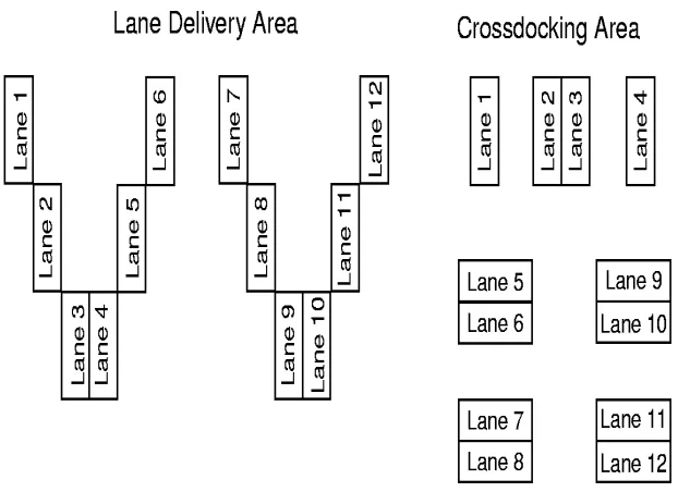
3. A layout consisting of two V shaped areas, one for lanes 1-6 and one for lanes 7-12. In the middle of each area, a lane for the CP is created. The third new layout assumes that the supplier will divide the CP into boxes with destination 1-6 and 7-12 to make crossdocking easier. The layout is shown in Figure 3.3.

(41)

to three rows of parts in a flowrack, with an overflow area to accept excess material in case all rows are occupied. In a proposed new layout, the material at the line will be reduced to only one row of parts per flowrack and there will be no overflow area. The assembly line team members will request additional material by internal Kanban cards. In the future layout, material with a low volume of containers per truckload and a high quantity of parts per container will be handled in the lane area; material with a high volume of containers per truckload and a low quantity per container will be stored intermittently in either flowracks or a designated floor space. Depending on container size, about 50% of the parts will be stored in flowracks/floor space . The parts will be picked from this area using dollies, which will then wait for the line delivery. The lane storage area will handle the remaining 50% and will be rearranged. Each lane will ini-tially handle the material for two lines, and the final separation will take place during the crossdocking process. After crossdocking, the dollies will go to the same area as the dollies with the parts picked from the flowracks/floorspace, and they will be de-livered to the lane together. Toyota’s proposed new layout is illustrated in Figure 3.4. The terms future layout and Toyota’s proposed new layout are used interchangeably for the remainder of the dissertation.

3.3 Research Questions

The research question that will be answered in the simulation portion of this study are:

• Research Question 1: Do differences in the percentage of pallets that have to be cross-docked have a significant effect on the workload of the team members?

• Research Question 2: Do differences in lane layout organization have a significant effect on the workload of the team members?

• Research Question 3: Do differences in the volume of incoming parts have a significant effect on the workload of the team members?

3.4 Parameters

(42)

Assembly Line Area

Lane 1/2 Lane 3/4 Lane 5/6 Lane 7/8 Lane 9/10 Lane 11/12

Pit 1 Pit 2 Pit 9 Pit 10

12 x 5 dollies for line delivery

floor space for full pallets

flowracks for boxes 12 x 3 dollies for crossdocking

(43)

1. Percentage of crossdocking pallets

An analysis of the current and future truck schedule will determine both the current and future average percentage level of pallets to be crossdocked. If there is a practical significant difference (more than 5%) in the two percentage levels both will be used for the simulation runs. In addition, after calculating the current and future percentages, one additional percentage level of crossdocking activity will be determined. This will allow a generalization of the results of the study to a wider variety of JIT companies. 2. Layouts

The existing layout, the three newly designed layouts and the proposed future layout as described earlier will be simulated and compared.

3. Volume of incoming parts

The data available at TMMK for the incoming parts is divided into 20 minute time intervals. Each time interval contains information about the number of boxes per sup-plier in this interval. The information on how many pallets these parts come in is not available, but Toyota requires suppliers to group parts by lane when building the pallets. From that requirement, an algorithm was developed to “arrange” the existing data into pallets. A flowchart of the algorithm is illustrated in Figure 3.5. This algo-rithm does not give the optimal arrangement of boxes on the pallets, which is itself an NP-complete problem, but it mimics the behavior of the logistic people at the supplier plant, who most likely are not using a sophisticated optimization technique to build the pallets. A distribution function will be fitted to the current and future (50% reduced) volume of incoming pallets and then used for the simulation runs.

A total of 30 simulations ( 3 levels of CP x 5 layouts x 2 volumes of incoming parts) will be run and analyzed. Table 3.1 provides an overview about all possible combinations of the three parameters.

Table 3.1: Possible combinations of the three simulation parameters

% CD Quantity Original Layout New Layout 1 New Layout 2 New Layout 3 Future Layout Current Current

Future Current New Current Current Future

(44)

# = number of incoming boxes;

each pallet has on average 12.5 boxes;

** loop1 read all records, write all full

pal-lets into new file, delete the records out of the old file do until end of file;

start loop1;

if # > 11.5 and < 12.5 --> 1 pallet; if # > 12.5 x = # / 12.5

--> x pallets, remainder ----> new #; end loop1;

** loop2 “build” pallets do until supplier changes; start loop2;

sort all records by quantity; if first # > 6.5

loop 3 ** read first # and find

an-other

pal-let so that the sum is closest to 12.5 add first # and last #; if sum < 12.5 --> 1 pallet;

if sum > 12.5 --> sub 1 last, goto loop3; end loop3

if first # < 6.5 loop 4

add first # and next #;

if sum > 12.5 --> sub next #, first # --> 1 pallet;

if sum < 12.5 --> add next, goto loop 4; end loop4;

end loop2;

(45)

3.5 Performance Measures

The workload for the truck drivers is defined as the sum of the driving distances between the pits and the lanes. Because the main objective of this study is the optimization of the crossdocking area, the workload of the truck drivers is not considered. The workload for the crossdocking team members is defined as the distance they have to walk to transport the boxes from one lane to another. The main workload of the line delivery people is the unloading of the boxes at the workstations. Because the unloading process is not influenced by the new layouts, it will not be considered as a performance measure.

3.6 The Simulation Model

Experimentation with a real world system is expensive and, in most cases, not practical. In our case, it would mean changing the layout of the lane, observing its performance for a week or month, and risking a shut down of the assembly line should the crossdocking not be done effectively and parts unable to be delivered to the workstation on time. In addition, only the current volume of incoming parts and percentage of CP could be tested. In simulations, on the other hand, testing different scenarios requires only an adjustment of the simulation model, and it is a lot faster since only the actual events are simulated. Therefore, simulation is a much more economical solution.

A discrete event simulation model will be created using ARENA. ARENA uses a graphical user interface (GUI) for SIMAN, a general purpose simulation language providing subrou-tines for event timing, file handling, and statistical calculations. The GUI speeds up the development of the model and the animation makes it easy for end users, such as the logis-tics manager, to understand. The simulation model is described in the next section.

3.6.1 Details of the Simulation Model

(46)

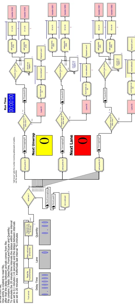
of a pallet if the parts have to be crossdocked. The record contains 3 fields: DelayTime, FromLaneToLane and Quantity. The DelayTime field mimics the 20 minute time intervals, with the first record starting with time 0 and each subsequent record in the same time interval containing 1 second. The next time interval starts at 20 minutes minus the number of seconds used for the preceding time interval. The field FromLaneToLane contains the information on the lane to which the parts belong and, if they have to be crossdocked, to which lane the parts should ultimately go. An entry of 0204 would mean the parts first go to lane 02 and from there they are crossdocked to lane 04. The quantity field contains the number of boxes on the pallet.

After reading the file, the next step is to determine in which lane the parts belong and to separate the parts into the lanes. A submodel is used to model the unwrapping process. One challenge in the modeling process was to realistically simulate the behavior of the team members in the crossdocking area. In reality, the team member would determine the lane that has the most pallets in it and unwrap all pallets for that lane, independent of the fact that in the meanwhile, another lane has more waiting pallets. The simulation software, on the other hand would change the allocation of the resource (i.e., the team member) as soon as another lane has more parts waiting to be unwrapped. To solve this dilemma, two counters were needed; the moment a resource starts working on a particular lane, the number of waiting parts in that lane is recorded. Another counter adds the number of parts processed, and the resource does not get released until both numbers match. The submodel used to simulate the unwrapping part is shown in Figure 3.7. To determine which lane has to be processed next, another submodel, shown in Figure 3.8, was created to find the lane with the most parts waiting.

After the pallets are unwrapped, a decision is made as to whether the parts stay in the lane or have to be crossdocked. The crossdocking process takes place in another submodel, shown in Figure 3.9. This submodel uses the same logic to assure the transfer of all parts before the team member switches to another lane. One counter is used to store the sum of parts waiting to be transferred, and another counter is used to sum the transferred parts. If both match, the resource/team member is released and is able to work on the next lane. After all parts in one lane are transferred, the lane with the most parts waiting for transfer is determined, as shown in Figure 3.10, and processed.

(47)

T ru ck ar riv al ! "#$%!&"'!'() ) *& ) ar riv al tim e D el ay un til ac tu al O rig in al fo rA rr iv al du pl ic at e en tit y S ep ar at e in to w ha tl an e ? La ne == 01 La ne == 02 La ne == 03 La ne == 01 02 La ne == 01 03 La ne == 02 01 La ne == 02 03 La ne == 03 01 La ne == 03 02 no ta va lid pa rt ot he rl an e ? tra ns fe rf ro m 01 to T ru e Fa ls e tra ns fe r0 10 2 tra ns fe r0 10 3 ot he rl an e ? tra ns fe rf ro m 03 to Tru e Fa ls e D is po sa lL an e 1 tra ns fe r0 20 1 tra ns fe r0 20 3 D is po sa lL an e 2 ot he rl an e ? tra ns fe rf ro m 02 to Tru e Fa ls e tra ns fe r0 30 1 tra ns fe r0 30 2 D is po sa lL an e 3 ha pp en 2 sh ou ld no t ? tra ns fe rf ro m 02

to Lane

== 02 01 La ne == 02 03 Els e Tr uc kS ch ed ul e R ea d fil e ha pp en 3 sh ou ld no t ? tra ns fe rf ro m 03

to Lane

== 03 01 La ne == 03 02 E ls e 02 01 ad d qu an tit y 02 03 ad dq ua nt ity 03 01 ad d qu an tit y 03 02 ad d qu an tit y + ,-,./0//& %! ' ( ad d qu an tit y 01 ad d qu an tit y 02 ad d qu an tit y 03 Unwrapping01 La ne 01 La ne 02 La ne 03 Unwrapping02 Unwrapping03 NextUnwraptest _NextLane01 ? tra ns fe rf ro m 01

to Lane

== 01 02 La ne == 01 03 Els

e happ

en 1 sh ou ld no t 01 02 ad d qu an tit y 01 03 ad d qu an tit y m ov e do lli es 01 01 to 02 01 to 03 Transfer01 _Transfer02 m ov e do lli es 02 02 to 01 02 to 03 03 to 01 03 to 02 Transfer03 m ov e do lli es 03 01 S um bo xe s ou t 02 S um bo xe s ou t 03 su m bo xe s ou t 0 0 0 00 :0 0: 00 0 0 0 0 0 0 0 0 0 0

0

0 0

0

0.

00

0

0.

00

0

0 0 0 0 0

0 0 0 0

0

(48)

Dollies

UW1 Store True

False UW1 Next Unwrapping

Unwrap UW1 Delay storeduw

UW1 add counter

sub stored

UW1 add unwrap UW1 unwrap lower total True

False

unwrap and totalUW1 clear

Unwrapping of pallets and moving dollies to line delivery area

NextUnwrap01

Submodel: Unwrapping

UW1 Unwrap _MoveDolliesUW1

0

0 0

Figure 3.7: Submodel: Unwrapping

NU1 which unwrap next

StoredUW01>=StoredUW02 .and. StoredUW01>=StoredUW03 StoredUW02>=StoredUW01 .and. StoredUW02>=StoredUW03 StoredUW03>=StoredUW01 .and. StoredUW03>=StoredUW02 Else

NextUnwrap01NU1

NextUnwrap02NU1

to totaluw01 NU1 storeduw01

to totaluw02 NU1 storeduw02

NextUnwrap03NU1 NU1 storeduw03to totaluw03 happen

NU1 should not

Which lane has to be unwrapped next ?

0

(49)

sumboxes stored and TF01 add counter

TF01 S tore

stored

processed subTF01 add

total

processed andTF01 clear NextLane01

TF01 Lane 01 next ?

True

False

TF01 Delay

total

TF01 process smaller True

False

Submodel: Tr ansfer

W hich lane shoul d be transferred next?

0

Figure 3.9: Submodel: Transfer

Sub1 which lane next

Stored01>=Stored02 .and. Stored01>=Stored03 Stored02>=Stored01 .and. Stored02>=Stored03 Stored03>=Stored01 .and. Stored03>=Stored02 Else

NextLane01Sub1

happen Sub1 should not

NextLane02Sub1

total01 Sub1 stored01 to

total02 Sub1 stored02 to

NextLane03Sub1 Sub1 stored03 tototal03

Submodel: Next lane

Which lane has to be transferred next ?

0

(50)

Besides the main model, two additional models are used. After 10 minutes of simulated time, the first model sets the lane that has to be unwrapped first. The other model is used to simulate the end of the shift when no more parts are coming in. The two models are shown in Figures 3.11 and 3.12.

C reate 7 which unwrap first

S toredUW01>=StoredUW02 .and. S toredUW01>=StoredUW03 S toredUW02>=StoredUW01 .and. S toredUW02>=StoredUW03 S toredUW03>=StoredUW01 .and. S toredUW03>=StoredUW02 E lse

F irst Unwrap01

happen should not F irst unwrap NextUnwrap02

F irst

totaluw01 storeduw01 to

F irst

to totaluw02 F irst stored02

NextUnwrap03 F irst

totaluw03 storeduw03 to

F irst

Start: A fter 10 minutes determine which lane to unwrap first

0

Figure 3.11: Model: Which lane to unwrap first

3.7 Current Toyota Data

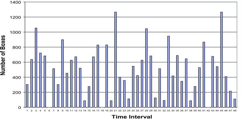
The original data, provided by Toyota’s logistics department, contained the number of in-coming boxes per supplier per line segment (overall 35) divided into 20 minute intervals. Because this study is interested in the number of boxes per lane per time interval, the differ-ent line segmdiffer-ents and suppliers are added up to the number of containers per lane, as shown in Table 3.2 and Figure 3.13. There is no obvious pattern in the data; three time buckets have no incoming parts at all, whereas two time buckets have over 1260 incoming parts. On average, 508.26 parts come in during a 20 minute time period, with a high variance of 106568.

(51)

C reate 6 which lane first

S tored01>=Stored02 .and. S tored01>=Stored03 S tored02>=Stored01 .and. S tored02>=Stored03 S tored03>=Stored01 .and. S tored03>=Stored02 E lse

First NextLane01

happen First should not First NextLane02

total01 First stored01 to

First NextLane03

S tart: Determine which lane to transfer last

0

Figure 3.12: Model: End of simulation

Table 3.2: Number of boxes per 20 minute interval for current data

Interval 21 45 3 28 33 9 41 19 17 4 35 5 29 43 12 16

# of Boxes 1266.47 1266.47 1053.87 1045.64 946.91 898.86 867.55 829.65 828.44 722.57 689.54 683.62 683.62 676.88 671.71 671.39

cum 1266.47 2532.94 3586.81 4632.45 5579.36 6478.22 7345.77 8175.42 9003.86 9726.43 10415.97 11099.59 11783.21 12460.09 13131.80 13803.18

% 5.19 5.19 4.32 4.29 3.88 3.68 3.56 3.40 3.40 2.96 2.83 2.80 2.80 2.77 2.75 2.75

cum % 5.19 10.38 14.70 18.99 22.87 26.55 30.11 33.51 36.91 39.87 42.69 45.50 48.30 51.07 53.83 56.58

Interval 37 2 27 11 25 44 40 13 7 31 10 26 34 46 22 23

# of Boxes 645.75 635.98 627.66 627.04 546.28 541.83 527.88 520.44 514.33 514.33 453.82 423.24 418.27 408.80 400.55 358.10

cum 14448.94 15084.92 15712.58 16339.61 16885.89 17427.72 17955.60 18476.04 18990.37 19504.71 19958.52 20381.76 20800.03 21208.83 21609.37 21967.47

% 2.65 2.61 2.57 2.57 2.24 2.22 2.16 2.13 2.11 2.11 1.86 1.73 1.71 1.68 1.64 1.47

cum % 59.23 61.83 64.41 66.98 69.21 71.44 73.60 75.73 77.84 79.95 81.81 83.54 85.26 86.93 88.58 90.04

Interval 36 1 8 15 39 47 30 24 48 32 14 20 38 6 18 42

# of Boxes 346.08 303.84 303.63 277.67 277.67 215.37 125.31 112.94 110.42 90.88 88.36 88.36 88.36 0.00 0.00 0.00

cum 22313.55 22617.39 22921.02 23198.68 23476.35 23691.72 23817.03 23929.97 24040.39 24131.27 24219.63 24307.98 24396.34 24396.34 24396.34 24396.34

% 1.42 1.25 1.24 1.14 1.14 0.88 0.51 0.46 0.45 0.37 0.36 0.36 0.36 0.00 0.00 0.00

(52)

0 200 400 600 800 1000 1200 1400

1 2 3 4 5 6 7 8 9 10 11 12 13 14 15 16 17 18 19 20 21 22 23 24 25 26 27 28 29 30 31 32 33 34 35 36 37 38 39 40 41 42 43 44 45 46 47 48

Time Interval

N

um

be

r

of

B

ox

es

Figure 3.13: Number of boxes per 20 minute interval for current data

Table 3.3: Cumulative data per lane for current data

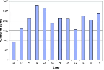
Lane # of Boxes % cum cum%

04 2779.77 11.39 2779.77 11.39

05 2639.16 10.82 5418.93 22.21

12 2377.67 9.75 7796.60 31.96

10 2241.34 9.19 10037.94 41.15

03 2128.93 8.73 12166.87 49.87

07 2125.36 8.71 14292.23 58.58

08 2109.15 8.65 16401.38 67.23

11 2041.64 8.37 18443.02 75.60

06 1879.33 7.70 20322.35 83.30

02 1612.53 6.61 21934.88 89.91

09 1552.88 6.37 23487.76 96.28

(53)

0 500 1000 1500 2000 2500 3000

01 02 03 04 05 06 07 08 09 10 11 12

Lane

N

u

m

b

e

r

o

f

B

o

x

e

s

(54)

A matrix with all possible lane combination for the crossdocking parts and the number of boxes that flow between them is shown in Table 3.4. From the 24396 parts 1784 or 7.31% have to be crossdocked.

Table 3.4: Flowmatrix for current data

exit 01 02 03 04 05 06 07 08 09 10 11 12

01 785.21 56.40 4.76 7.92

02 40.01 1502.77 13.20 7.52 31.57 3.13 48.66 45.75 19.79 40.49

03 1877.12 14.30 25.00 12.74 50.44

04 5.30 2547.58 8.40 61.53 43.01 2.48

05 20.50 2460.22 80.00 16.30 7.86

06 19.77 47.33 1867.84 30.51 8.52 80.92 1.58

07 4.36 24.80 2.42 2096.50 39.73

08 16.70 12.22 1861.89

09 20.54 4.94 15.99 13.53 29.09 1487.58 31.83 9.16 35.07

10 26.99 35.33 42.28 13.26 68.48 5.94 7.72 66.56 2028.25 28.70 2.12

11 26.75 14.87 53.89 89.33 14.59 27.95 1882.44 33.00

12 9.09 32.62 13.20 42.16 2.79 10.29 2214.97

3.8 Toyota Data for the Proposed Changes

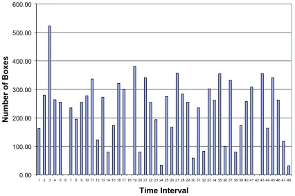
The proposed changes lead to a reduction of roughly 50% in the number of boxes that are handled in the crossdocking area, the other 50% are stored into the newly created flowracks. The new quantities per 20 minute bucket are shown in Table 3.5 and Figure 3.15.

Table 3.5: Number of boxes per 20 minute interval for data from Toyota’s proposed changes

Interval 3 19 27 43 35 21 45 11 37 16 41 33 17 28 2 10

# of Boxes 522.98 380.72 356.76 355.16 354.59 341.15 341.15 336.48 331.34 321.01 308.10 301.88 298.68 283.38 279.73 277.36

cum 522.98 903.70 1260.46 1615.62 1970.21 2311.36 2652.51 2988.99 3320.33 3641.34 3949.43 4251.31 4549.98 4833.36 5113.09 5390.45

% 4.99 3.63 3.40 3.39 3.38 3.25 3.25 3.21 3.16 3.06 2.94 2.88 2.85 2.70 2.67 2.65

cum % 4.99 8.62 12.02 15.41 18.79 22.05 25.30 28.51 31.67 34.74 37.68 40.56 43.40 46.11 48.78 51.42

Interval 25 13 4 46 34 40 5 29 9 22 7 31 8 23 15 39

# of Boxes 274.70 272.70 263.54 262.56 261.61 257.37 255.08 255.08 254.49 254.31 234.77 234.77 194.88 193.39 173.10 173.10

cum 5665.15 5937.85 6201.39 6463.94 6725.55 6982.92 7238.00 7493.09 7747.58 8001.89 8236.66 8471.43 8666.31 8859.70 9032.80 9205.91

% 2.62 2.60 2.51 2.50 2.50 2.46 2.43 2.43 2.43 2.43 2.24 2.24 1.86 1.84 1.65 1.65

cum % 54.04 56.64 59.16 61.66 64.16 66.61 69.05 71.48 73.91 76.33 78.57 80.81 82.67 84.52 86.17 87.82

Interval 26 44 1 12 47 36 32 14 20 38 30 24 48 6 18 42

# of Boxes 167.21 163.39 162.18 121.96 117.33 99.57 82.36 79.83 79.83 79.83 58.64 33.59 31.06 0.00 0.00 0.00

cum 9373.12 9536.51 9698.69 9820.65 9937.98 10037.55 10119.91 10199.74 10279.57 10359.40 10418.04 10451.63 10482.69 10482.69 10482.69 10482.69

% 1.60 1.56 1.55 1.16 1.12 0.95 0.79 0.76 0.76 0.76 0.56 0.32 0.30 0.00 0.00 0.00

cum % 89.42 90.97 92.52 93.68 94.80 95.75 96.54 97.30 98.06 98.82 99.38 99.70 100.00 100.00 100.00 100.00

(55)

0.00 100.00 200.00 300.00 400.00 500.00 600.00

1 2 3 4 5 6 7 8 9 10 11 12 13 14 15 16 17 18 19 20 21 22 23 24 25 26 27 28 29 30 31 32 33 34 35 36 37 38 39 40 41 42 43 44 45 46 47 48

Time Interval

N

u

m

b

e

r

o

f

B

o

x

e

s

(56)

the reduced quantities per lane as of the proposed changes. The reduction is not distributed equally over all lanes, lane 1 has only a 4 % reduction whereas lane 4 has nearly a 75 % reduction.

Table 3.6: Cumulative data boxes per lane for data from Toyota’s proposed changes

Lane # of Boxes % cum cum%

05 1232.62 11.76 1232.62 11.76

11 1181.45 11.27 2414.07 23.03

03 1094.59 10.44 3508.66 33.47

07 1072.37 10.23 4581.03 43.70

08 1059.30 10.11 5640.33 53.81

10 913.01 8.71 6553.34 62.52

01 871.97 8.32 7425.31 70.83

04 703.42 6.71 8128.73 77.54

12 669.89 6.39 8798.62 83.93

06 665.60 6.35 9464.22 90.28

02 627.66 5.99 10091.88 96.27

09 390.81 3.73 10482.69 100.00

The quantities that have to be crossdocked between the lanes are illustrated in Table 3.7. From the 10482 parts 1577 or 15.04% have to be crossdocked.

Table 3.7: Flowmatrix for data from Toyota’s proposed changes

to

from 01 02 03 04 05 06 07 08 09 10 11 12

01 684.20 24.14 33.00 5.54 14.87 13.20 27.29

02 488.68 20.91 16.05 6.09

03 7.86 879.10 13.20 10.42 8.73 18.18

04 1.13 61.80 603.69 45.63 51.33 12.60 29.64

05 22.30 1160.78 21.60 6.82 52.69

06 4.16 29.25 20.36 495.25 0.73 6.37 15.18 10.92

07 32.57 50.44 11.13 868.77 27.28 27.20

08 1.58 30.78 47.33 63.56 989.78 8.52

09 16.08 9.41 40.49 20.69 17.16 323.17 29.48 35.53 19.79

10 105.14 42.48 7.27 58.59 17.49 9.35 14.03 794.85 1.90 5.30

11 16.50 9.57 38.97 19.80 12.41 7.90 1053.02 21.82

(57)

0 200 400 600 800 1000 1200 1400

1 2 3 4 5 6 7 8 9 10 11 12

Lane

N

u

m

b

e

r

o

f

B

o

x

e

s

(58)

1 ₂

3 ₄

5 ₆

7 ₈

9 ₁₀

11 ₁₂

0 500 1000 1500 2000 2500 3000

N

u

m

b

e

r

o

f

B

o

x

e

s

Lane

Data from Toyota's Proposed Changes Current Data

SIMULATION AND OPTIMIZATION OF A CROSSDOCKING OPERATION IN A JUST-IN-TIME ENVIRONMENT

UKnowledge

UKnowledge

SIMULATION AND OPTIMIZATION OF A CROSSDOCKING

SIMULATION AND OPTIMIZATION OF A CROSSDOCKING

OPERATION IN A JUST-IN-TIME ENVIRONMENT

OPERATION IN A JUST-IN-TIME ENVIRONMENT

Contents

List of Figures

List of Tables

List of Files

Chapter 1

Introduction

1.1

Statement of the Problem

1.2

Description of the Lane Storage Area at Toyota

1.3

Research Goals and Contribution

Chapter 2

Literature Review

2.1

Review of JIT Delivery Literature

2.2

Review of Mixed-Model Assembly Line Literature

2.3

Review of Crossdocking Literature

2.4

Review of Facility Layout Studies

2.4.1

The Facility Layout Problem and the Quadratic Assignment

Prob-lem Approach

2.4.2

Special Layout Cases

Chapter 3

The Simulation Study

3.1

Definitions

3.2

Layouts Simulated

3.3

Research Questions

3.4

Parameters

3.5

Performance Measures

3.6

The Simulation Model

3.6.1

Details of the Simulation Model

0

0

0.

00

00

0

0.

00

0

Which lane has to be unwrapped next ?

Submodel: Next lane

Which lane has to be transferred next ?

Start: A fter 10 minutes determine which lane to unwrap first

3.7

Current Toyota Data

3.8

Toyota Data for the Proposed Changes