Modelling of Lake Water Quality Parameters by Deep Learning Using Remote Sensing Data

Modelling of Lake Water Quality Parameters by Deep

Learning Using Remote Sensing Data

Randrianiaina Jerry J. C. F.*, Rakotonirina Rija I., Ratiarimanana Jean R., Lahatra Razafindramisa Fils

University of Antananarivo, Science and Technology Domain, Physics Department, Laboratory of Matter and Radiation Physics (LPMR), Madagascar

Abstract

The modelling of lake water quality is very important to make some prediction and to monitor it. Modelling Lake water quality, utilizing the data obtained from the in-situ measurements, collecting samples from the in situ and analyzing them in a laboratory are very expensive and time consuming. Several algorithms can be used to model lake water quality using the in-situ measurements data. In this work, Deep Learning was used to perform pH, dissolved oxygen, conductivity and turbidity modelling of the Itasy Lake. Deep Learning is another branch of machine learning or automatic training that works well to solve many problems. The obtained results demonstrated that the developed model of a deep neural network (deep learning) provides an excellent relationship between the observed and simulated water quality parameters. Moreover, the coefficient of correlation (R2) was 0.89 for pH, 0.97 for the dissolved oxygen, 0.96 for the conductivity and 0.99 for the turbidity. The root mean square error (RMSE) values for pH, dissolved oxygen, conductivity and turbidity were below 0.22, 0.21 mg.l-1, 1.37 µS.cm-1, and 0.53 NTU respectively, during the deep learning training and validation phases. After getting the model, the parameters of the Itasy Lake water were estimated on 1st January 2019. The obtained results are as follows: pH was ranged from 7.1 to 7.6, 7.0 mg.l-1 to 7.2 mg.l-1 for the dissolved oxygen, 55.7 µS.cm-1 to 57.1 µS.cm-1 for the conductivity and 12.0 to 12.2 NTU for the turbidity. It was shown that the water quality of Itasy respects the Malagasy norm with regard to pH, dissolved oxygen, conductivity and turbidity. And the mean values for these parameters were respectively 7.6 for pH, 7.01 mg.l-1 for the dissolved oxygen, 57.05 µS.cm-1 for the conductivity and 12.03 NTU for the turbidity.

Keywords

Remote sensing, GIS, Landsat8, Deep Learning, Water Quality, Itasy Lake, Madagascar

1. Introduction

Lake water is one of the most important basic resources of the biodiversity on the Earth. Water is essential for the existence, development, preservation of human life (Kanniyappan, S. P. et al., 2016) and aquatic life. Therefore, the modelling, monitoring and the study of its quality are very important to preserve and to protect this resource. Several techniques could be used to determine and monitor water quality (including physical, chemical and biological parameters properties), such as in-situ measurements, sample collection from the site and laboratory analyses. These methods are very expensive and time consuming. Moreover, time and cost constraints associated with in-situ measurements of lake water quality often limit the assessment of spatial and temporal trends of water quality

* Corresponding author:

[email protected] (Randrianiaina Jerry J. C. F.) Published online at http://journal.sapub.org/ajgis

Copyright©2019The Author(s).PublishedbyScientific&AcademicPublishing This work is licensed under the Creative Commons Attribution International License (CC BY). http://creativecommons.org/licenses/by/4.0/

(Panda S.S. et al, 2004). This study tried to propose a solution to these problems. The remote sensing technique was used, coupled with Geographic Information System (GIS), which is nowadays the main technique used for detecting, modelling and monitoring water quality. Many water quality parameters can be detected, modelled and monitored from this technique. In this research, the quality parameters that were detected are pH, dissolved oxygen, conductivity and turbidity. The main objective of the study was to model these four quality parameters for Lake Itasy using the Deep Learning algorithm.

remote sensing. Thus, the application of electromagnetic radiation detection can be extended to surface water survey because the backscattering characteristics of waves depend on the types and concentrations of substances in the water (Shubha, 2000). The visible (blue, green, red) and infrared spectral bands were chosen, because the spectral response for these bands has a relationship with water quality.

2. Study Area and Data Used

2.1. Study Area

The study area is situated in the center part of Madagascar, in the region of Itasy. The Itasy Lake is among the continental lakes of Madagascar, sited within the volcanic field of Itasy and geographically located between 19°04’ latitude South and 46°47’ longitude East (Figure 1).

Figure 1. Located of study area

2.2. Data Used

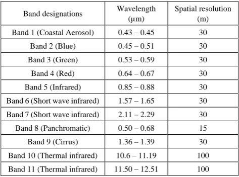
Table 1. Landsat 8 characteristics (Landsat 8 Data Users Handbook, 2016)

Band designations Wavelength

(µm)

Spatial resolution (m)

Band 1 (Coastal Aerosol) 0.43 – 0.45 30

Band 2 (Blue) 0.45 – 0.51 30

Band 3 (Green) 0.53 – 0.59 30

Band 4 (Red) 0.64 – 0.67 30

Band 5 (Infrared) 0.85 – 0.88 30

Band 6 (Short wave infrared) 1.57 – 1.65 30

Band 7 (Short wave infrared) 2.11 – 2.29 30

Band 8 (Panchromatic) 0.50 – 0.68 15

Band 9 (Cirrus) 1.36 – 1.39 30

Band 10 (Thermal infrared) 10.6 – 11.19 100

Band 11 (Thermal infrared) 11.50 – 12.51 100

Satellite images at path 159 and row 073 from landsat8 were the main data used in this work. Landsat8 data images at L1T-Orthorectified can be downloaded freely from the website of USGS or United States Geological Survey (https://earthexplorer.usgs.gov). Landsat8 was launched on

11 February 2013 ensuring the mission continuity of Landsat data at a high spatial resolution but normal operations began on 30 May 2013. Landsat8 carries two sensors OLI (Operational Land Imager) and TIRS (Thermal Infrared sensors) on board. OLI have nine spectral bands over 190 km swath, with 30 m spatial resolution for the eight bands and one panchromatic band at 15 m. TIRS are at a 100 m spatial resolution using two bands between 10-12 µm. The characteristics of Landsat 8 OLI/TIRS are given in Table 1.

3. Water Quality Parameters (WQPs)

Four water quality parameters were modelled with Deep Neural Network in this study to determine the Itasy Lake water quality: pH, Dissolved Oxygen, Conductivity and Turbidity.

3.1. pH

Hydrogen potential or pH is one of the most important chemical parameters for the determination of water quality. pH values are greatly sensitive to the water contamination. Therefore, pH is considered as an indicator of water pollution. It characterizes the acidity and the alkalinity of the water. pH is measured on a scale of 0 to 14. Water that is neutral has a pH of 7. Acidic water has pH values less than 7, with 0 being the most acidic and basic water has pH values greater than 7, with 14 being the most basic. A change of 1 unit on a pH scale represents a 10 fold change in the acidity, thus water with a pH of 6 is 10 times more acidic than water with a pH of 7, and water with a pH of 5 is 100 times more acidic than water with a pH of 7 (Nancy Mesner and John Geiger, 2005).

3.2. Dissolved Oxygen

Dissolved oxygen (D.O), often called the oxygen demand (O.D), is also one of the important parameters in the determination and assessment of water quality. D.O is essential for an aquatic ecosystem since it controls the biological productivity (Prasad B.S.R.V. et al., 2014), ensures and protects the aquatic life (Randrianiaina Jerry J.C.F. et al., 2018). The level of dissolved oxygen in the water is one of the major parameters in determining its quality for it indirectly indicates whether there is some kind of pollution (Jorge G. Ibanez et al., 2008). D.O is measured as part per million (ppm) or its equivalent, milligrams per liter (mg.l-1). D.O concentration is influenced by replenishment rates (contribution from aerated tributary streams, surface exchange with the atmosphere, amount of aquatic photosynthesis) and consumption factors (respiratory demands of lake organisms, amount of oxygen demanding wastes) (Dr Bruce A. Gilman).

3.3. Conductivity

assess the purity of water (Murugesan A. et al., 2011), i.e. an indirect measure of ion content in water. It is evolved that the more water contains ions as calcium (Ca2+), magnesium (Mg2+), sodium (Na2+), potassium (K+), bicarbonate (HCO3-),

sulphate (SO42-) and chloride (Cl-), the more it can drive

electric current and the more conductivity is at high level. Conductivity is measured in the conventional unit called micro-Siemens per centimeter (µS.cm-1).

3.4. Turbidity

Water turbidity, an optical property of water, scatters and absorbs the light rather than transmitting it in straight lines (Mohammad H.G. et al., 2016). It can harm fish and other aquatic organisms by reducing feed supplies, degrading spawning grounds, and affecting gill function (Minnesota Pollution Control Agency, 2008). Turbidity is also a significant parameter for water quality and can be used as a surrogate for water clarity fixing (turbidity measured by the reflection of a light ray in the water). It is measured using an optic test which determines the capacity of reflecting light. The usual unit to measure turbidity is NTU (Nephelometric Turbidity Unity).

4. Methodology

4.1. Image Pre-Processing

The electromagnetic signals that a satellite sensor records are unsettled by atmosphere. An atmospheric correction was necessary to reduce the atmospheric effects in the Earth reflectance acquisition. For any remote sensing approach, atmospheric correction is thus required to minimize the atmospheric effects and to convert digital numbers (DN) to reflectance values (Hieu Cong Nguyen et al., 2015). The Dark Object Subtraction (DOS1) method was used in this work to remove atmospheric distortion effects and to calculate surface reflectance values. This method is well accepted by the geospatial community and can provide accurate mapping for wetland areas (Song C. et al., 2001).

4.1.1. DOS1 Radiance Correction

The atmospheric scattered radiance often called path radiance is given by Equation 1 (Sobrino, J. et al, 2004).

% 1 min







p





₍₁₎ where: ρp is the path radiance, ρmin the radiance that corresponds to the digital count value for which the sum of all the pixels with digital counts lower or equal to this value is equal to the 0.01% of all pixels from the image, and ρ1% is the radiance of the dark object, assumed to have a reflectance value of 0.01. The ρmin and ρ1% are given by Equation 2 and Equation 3 respectively.

L

L DN A

M 

 min

min *

 (2)

where:

ML: band-specific multiplicative rescaling factor from

metadata,

DNmin: DN minimum value,

AL: band-specific additive rescaling factor from the

metadata. ² ) cos( [ * 01 . 0 * % 1 d T E sT

ESUN Z down v

 

    ₍₃₎

where:

ESUNλ:the solar exoatmospheric spectral irradiances,

TZ: the atmospheric transmittance in the viewing direction,

Edown: the downwelling diffuse irradiance,

Tv: the atmospheric transmittance in the illumination

direction,

d:Earth-Sun distance

Yet, in the DOS1 atmospheric correction, Tv=1, Tz=1 and

Edown=0. By injecting the Equation (2) and (3) into Equation

(1), DOS1 radiance is finally given by (Equation 4): ² * )] cos( * 01 . 0 [ * min * d s ESUN A DN

ML L

p





     ₍₄₎

With ' ' * ² * p L M M d

ESUN ₍₅₎

ML’ and Mp’ were radiance maximum band X, from the metadata (where X is the band number) and reflectance maximum band X from the metadata (where X the band number).

4.1.2. DOS1 Reflectance Correction

DOS1 surface reflectance is given by Equation (6)

* [ ]

*cos( ) p

S

d L L

ESUN      

 (6)

Where Lλ is the spectral radiance at sensor’s aperture

given by Equation 7 (ML is the band specific multiplicative rescaling factor from metadata, Qcal is the quantized and calibrated standard product pixel values (DN) and Ap is the band-specific additive rescaling factor from metadata).

p cal LQ A

M

L   (7)

4.2. Deep Learning

4.2.1. Introduction

Figure 2. Relation between artificial intelligence, Automatic training and Deep Learning

4.2.2. Deep Architecture

The deep learning architecture consists of multiple layers of non-linear representations (Zheng Yi Wu and Atiqur Rahman, 2017). In this work, the deep learning algorithm was adopted to model the non-linear relationship between Landsat 8 reflectance data, many hidden layers and the input layers (Figure 3). The methodology adopted to get water quality modelling is described as follows. The Deep learning based modelling and predicted were used.

- In situ measurements: The measurement of quality parameters in situ, called output desired (layers desired), was necessary to train the network to adjust the output estimate.

- Input data: The Landsat8 reflectance is the input layers. The input data and the in situ measurements are taken on

the same date.

Let us note that the input layers and the many hidden layers are connected by the weights.

- Dropout is a technique where randomly selected neurons are ignored during training. They are “dropped-out” randomly. This means that their contribution to the activation of downstream neurons is temporally removed on the forward pass and any weight updates are not applied to the neuron on the backward pass (Jason Brownlee, 2016).

- Modelling: This includes the process to developing model. In this research, ADAM optimization was used to develop the model.

Figure 3. Deep Neural Network Architecture (ex for the conductivity)

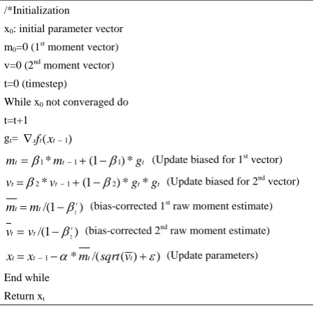
4.2.3. Optimization Algorithm

A method for stochastic optimization namely ADAM (Adaptive Moment Estimation) was utilized for training deep learning models i.e. to update network weights iterative in training data. ADAM is one of the algorithms that work well in range of deep learning architectures. The Algorithm 1, presented here, shows the Adam optimization.

Algorithm 1. Adam optimization for stochastic optimization

/*Initialization

x0: initial parameter vector

m0=0 (1st moment vector)

v=0 (2nd moment vector)

t=0 (timestep)

While x0 not converaged do

t=t+1

gt= xft(xt1)

t t

t m g

m 1* 1(11)* (Update biased for 1st vector)

t t t

t v g g

v2* 1(12)* * (Update biased for 2nd _vector)

) 1 /( 1

t

t

t m

m  (bias-corrected 1st _{raw moment estimate)}

) 1 /( 2

t

t

t v

v   (bias-corrected 2nd _{raw moment estimate)}

) ) ( /( *

1 

 t t t

t x m sqrt v

x (Update parameters)

End while

Return xt

4.2.4. Activation Function

In 2010, Nair and Hinton proposed a new activation function: the Rectified Linear Unit (ReLU) activation. ReLU has been the most widely used activation function for deep learning applications with state of the art results to date (Nair V. and Hinton G.E., 2010). It was a faster learning (LeCun et al., 2015), which has proved to be the most successful, widely used function (Ramachandran et al., 2017) and offers better performance and generalization in deep learning compared to the Sigmoid and tanh activation functions (Zeiler M. D. et al., 2013; Dahl G. E. et al., 2013). ReLU rectifies the inputs value less than zero thereby forcing them to zero and eliminating the vanishing gradient (Chigozie E. N. et al., 2018) thus ReLU is given by (Equation 8).

, 0

( ) max(0, )

0, 0

x if x

f x x and

if x

 



  

 _



(8)

5. Results and Discussion

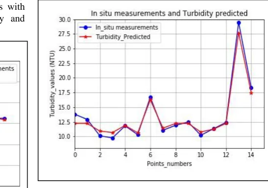
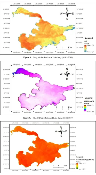
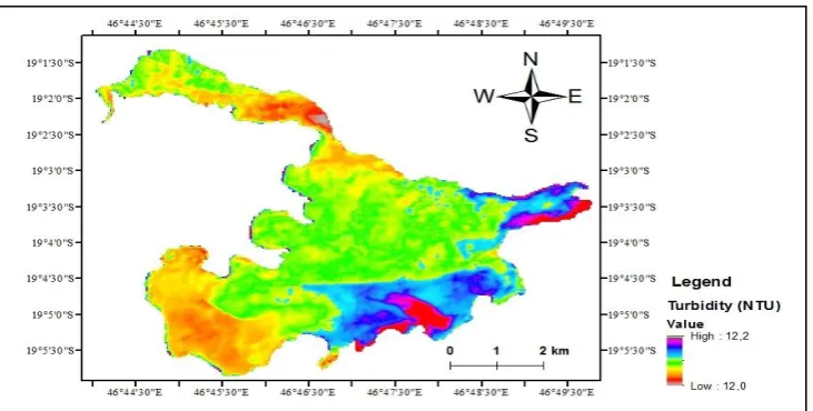
R2=0.97 for the dissolved oxygen, R2=0.96 for the conductivity and R2=0.99 for the turbidity. Moreover, the root mean square error (RMSE) values for pH, dissolved oxygen, conductivity and turbidity were below 0.22, 0.21 mg.l-1, 1.37 µS.cm-1, and 0.53 NTU respectively. After the model was built, it was applied to predict the water quality of the Itasy Lake using the remote sensing imagery collected on 1st January 2019, i.e. the new input data (new imagery) were introduced in the deep learning model, and the spatial distribution maps of pH, O.D, Conductivity and Turbidity shown in Figures 8, 9, 10 and 11 were obtained, these are the estimated values. The obtained mean values of the four parameters were respectively 7.6 for pH, 7.01 mg.l-1 for O.D, 57.05 µS.cm-1 for the conductivity and 12.03 NTU for the turbidity. The Malagasy decree n° 2003/464 issued on 15 April 2003 concerning water surface classification stipulates that if the pH range is between 6.0 and 8.5, the conductivity is less than 200 µS.cm-1, the O.D greater than 5 mg.l-1 and the turbidity inferior to 25 NTU, hence the lake water has good quality and the concerned lake is in good health. Therefore, it can be concluded that the Itasy Lake respects the norms dictated by the regulation.

6. Conclusion

These parameters that we modelled and estimate are the important parameters to survey lake water quality. Landsat surface reflectance was utilized combined with the in situ measurements values to perform the modelling of the water quality of the Itasy Lake surface using remote sensing. To show the performance of our model, the coefficient of correlation was used. This model reached a high level of coefficient of determination R² > 0.80 of all of these parameters, which is trustworthy. And after getting the model, the parameters of the Itasy Lake water were estimated on 1st January 2019. The obtained results show that Itasy Lake water parameters respect the Malagasy norms with regard to the pH, dissolved oxygen, conductivity and turbidity.

Figure 4. pH in-situ measurements and predicted

Figure 5. O.D in situ measurements and predicted

Figure 6. Conductivity in-situ measurements and predicted

Figure 8. Map pH distribution of Lake Itasy (01/01/2019)

Figure 9. Map O.D distribution of Lake Itasy (01/01/2019)

Figure 11. Map turbidity distribution of Lake Itasy (01/01/2019)

REFERENCES

[1] Chigozie E. N.; Winifred I.; Anthony G. and Stephen M. 2018. Activation Functions: Comparison of Trends Practice and Research for Deep Learning.

[2] Dahl, G. E.; Sainath, T. N. and Hinton, G. E. 2013. Improving deep neural networks for LVCSR using rectified linear units and dropout. International Conference on Acoustics, Speech and Signal Processing.

[3] Dr. Bruce A. Gilman, WATER QUALITY REPORTS, HEALTH OF CANANDAIGUA LAKE AND TRIBUTARY STREAMS.

[4] Hieu Cong Nguyen; Jaehoon Jung; Jungbin Lee; Sung-Uk Choi; Suk-Young Hong and Joon Heo. 2015. Optimal Atmospheric Correction for Above-Ground Forest Biomass Estimation with the ETM+ Remote Sensor. Sensors, vol. 15, n° 8, p. 18865-18886.

[5] Jason Brownlee. 2016. Deep learning.

[6] Kanniyappan, S.P.; Raguraj, D.P. and Vigneshwaran, E. 2016. Physico-Chemical Analysis of Ground and Surface Water in Cuddalore District due to Effect of 2015 Monsoon. Adv. Appl. Sci. Res., 7(4): 176-184.

[7] Landsat 8 Data Users Handbook, 2015. Retrieved March 29, from http://landsat.usgs.gov/documents/Landsat8DataUsers Handbook.pdf.

[8] LeCun, Y.; Bengio, Y. and Hinton, G. 2015. Deep learning. Nature, 521(7553): 436-444.

[9] Minnesota Pollution Control Agency. 2008. Turbidity: Description, Impact on Water Quality. Sources, Measures — A General Overview, USA.

[10] Mohammad, H. G.; Melesse, A.M.; Reddi, L. 2016. A Comprehensive Review on Water Quality Parameters Estimation Using Remote Sensing Techniques. Sensors, 16, 1298.

[11] Murugesan, A.; Ramu, A.; Kannan, N. 2006. Water quality assessment from Uthamapalayam municipality in Theni

District, Tamil Nadu. India Pollution Research 25: 163-166. [12] Nair, V. and Hinton, G.E. 2010. Rectified linear units

improve restricted boltzmann machines. Haifa, pp. 807–814.

[13] Nancy Mesner and John Geiger. 2005. What is pH?

Understanding Your Watershed.

[14] Panda, S.S.; Garg, V. and Chaubey, I. 2004. Artificial Neural Networks Application in Lake Water Quality Estimation Using Satellite Imagery. Journal of Environmental Informatics 4 (2) 65-74.

[15] Prasad, B. S. R. V.; Srinivasu, P. D. N; Sarada Varma, P.; Raman, A. V. and Santanu Ray. 2014. Dynamics of Dissolved Oxygen in Relation to Saturation and Health of an Aquatic Body: A Case for Chilka Lagoon, India. Journal of Ecosystems, vol. 2014, Article ID 526245, 17 pages, https://doi.org/10.1155/2014/526245.

[16] Ramachandran, P.; Zoph, B. and Le Q. V. 2017. Searching for Activation Functions. ArXiv, 2017.

[17] Randrianiaina Jerry, J.C.F.; Rakotonirina Rija, I.; Ratiarimanana Jean, R.; Lahatra Razafindramisa Fils. 2018. Temperature Retrieval of Lake Itasy Using Remote Sensing. Resources and Environment, 8(6): 241-244.

[18] Shubha, S. 2000. Remote sensing of ocean colour in coastal, and other optically complex, waters. International Ocean-Color Coordinating Group, Busan, South Korea. http://www.ioccg.org/reports/report5.pdf.

[19] Sobrino, J.; Jiménez-Muñoz, J. C. & Paolini, L. 2004. Land surface temperature retrieval from LANDSAT TM 5 Remote Sensing of Environment, Elsevier, 90, 434-440.

[20] Song, C.; Woodcock, C. E.; Seto, K. C.; Lenney, M. P. and Macomber, S. A. 2001. Classification and change detection using Landsat TM data: when and how to correct atmospheric effects. Remote Sensing of Environment, 75, pp. 230-244. [21] Zeiler, M. D.; Ranzato, M.; Monga, R.; Mao, M.; Yang, K.;

Le, Q. V. and Hinton G. E. 2013. On rectified linear units for speech processing. International Conference on Acoustics, Speech and Signal Processing. IEEE, pp. 3517–3521. [22] Zheng Yi Wu and Atiqur Rahman. 2017. Optimized Deep