arXiv:0901.4604v2 [q-fin.CP] 27 Apr 2009
NUMERICAL ANALYSIS AND MODELING Computing and Information
Volume 6, Number 4, Pages 000–000
LAPLACE TRANSFORMATION METHOD FOR THE BLACK-SCHOLES EQUATION
HYOSEOP LEE AND DONGWOO SHEEN
(Communicated by Yanping Lin)
Abstract. In this paper we apply the innovative Laplace transformation method introduced by Sheen, Sloan, and Thom´ee (IMA J. Numer. Anal., 2003) to solve the Black-Scholes equation. The algorithm is of arbitrary high con-vergence rate and naturally parallelizable. It is shown that the method is very efficient for calculating various option prices. Existence and uniqueness prop-erties of the Laplace transformed Black-Scholes equation are analyzed. Also a transparent boundary condition associated with the Laplace transformation method is proposed. Several numerical results for various options under vari-ous situations confirm the efficiency, convergence and parallelization property of the proposed scheme.
Key Words.Black-Scholes equation, basket option, Laplace inversion, parallel method, transparent boundary condition
1. Introduction
As stock markets have become more sophisticated, so have their products. The simple buy/sell trades of the early markets have been replaced by more complex financial options and derivatives. These contracts can give investors various oppor-tunities to tailor their dealings to their investment needs.
One of the main concerns about financial options is what the exact values of options are. For the simplest model in the case of constant coefficients, an exact pricing formula was derived by Black and Scholes, known as the Black-Scholes formula. However, in the general case of time and space dependent coefficients the exact pricing formula are not yet established, and thus numerical solutions have been used.
In order to describe an option price, let x, K, t and T denote the underlying asset price, the strike price, the time to maturity, and the expiry date of an option, respectively. As usual,σand rrepresent the volatility of the underlying asset and the risk-free interest rate of the market, respectively. In this paper, we assume thatσ andrdepend onxonly. Then a European option priceu(x, t) satisfies the Black-Scholes equation:
∂u ∂t −
1 2σ
2x2∂2u ∂x2 −rx
∂u
∂x+ru= 0, (x, t)∈(0,∞)×(0, T],
(1.1)
2000Mathematics Subject Classification. 91B02, 44A10, 35K50.
The research of HL was partially supported by 2007-C00001 and that of DS by KRF-2007-C00031. To appear in International Journal of Numerical Analysis & Modeling. .
where an initial condition u0(x) = u(x,0) is given by the initial contract of an
option. The basket option based onnassetsx= (x1, . . . , xn) satisfies
∂u ∂t −
1 2
n
X
i,j=1
aijxixj ∂
2u ∂xi∂xj −
n
X
i=1 rxi ∂u
∂xi
+ru= 0,
(1.2)
(x, t)∈(0,∞)n×(0, T],
where aij =Pnk=1σikσjk, with σij representing the corelation between the assets
xiand xj.
Several numerical methods have been used for solving the Black-Scholes equation, for example in [32, 28] and [10] and the references therein, one can find popular numerical schemes for option pricing. Usually the time marching methods such as forward Euler, backward Euler and Crank-Nicolson schemes are used with a suitable spatial discretization scheme. In spite of the popularity of these time marching methods, a critical drawback of these schemes is that they usually require as many time steps as spatial meshes to balance the errors arising from discretization. In particular, for the estimation of basket options of reasonable size, the usual time marching schemes seem to be too slow in practice since the cost of solving an elliptic system to advance to a next time step is usually expensive. It is thus highly desirable to solve as small a number of elliptic solution steps as possible as well as to apply a very fast elliptic solver.
In this paper, we will focus on minimizing the number of elliptic solution steps by proposing the Laplace transformation method for the Black-Scholes equation, which is also naturally parallelizable. It will be shown that our method can dramatically reduce the computing time compared to the time marching schemes. Suitable contours should be chosen in order to have very fast convergence, and for this, we will estimate the resolvent of the Black-Scholes equation. Also, an exact transparent boundary condition will be given at which the infinite spatial domain is truncated. There have been some related works in which the Laplace transformation method has been used, for instance in [7, 18, 25]. However, in these earlier papers the Laplace transformation method has been used to obtain the analytic solution of various options rather than to develop an efficient numerical scheme. In particular, in [18] the partial Laplace transformation is applied for American option pricing, and in [6, 24] the Mellin transformation which is similar to the Laplace transfor-mation is used to evaluate the analytic solution of an option. Related with Laplace transformation methods there are other approaches based on the so-calledH-matrix approach; for instance, see [8, 9], and so on. Also, high-dimensional parabolic prob-lems can be solved using sparse grids [11, 15, 16, 27]. Application of our Laplace transformation method using sparse grids to option pricing will also be interesting. Other approaches in the fast time-stepping methods can be found in [34, 20, 19].
2. The Laplace transformation and its inversion
We begin with the abstract setting of a parabolic type equation so that the proposed scheme can be applicable to various problems. Consider
∂u
∂t +Au=f, t∈(0.T]; u(0) =u0,
(2.1)
whereu0is a given initial function andAa spatial elliptic operator with its
eigen-values being located in the right half plane. (We added the source term f(x, t), which is not present in (1.1) or in (1.2), in order to describe our method in more general setting.) For eachzin the complex plane, recall that the standard Laplace transform in time of a functionu(·, t) is given by
b
u(·, z) :=L[u](z) =
Z ∞
0
u(·, t)e−ztdt.
Then the Laplace transformation of (2.1) is thus given in the form
zub+Aub = u0+fb(·, z), z∈Γ,
(2.2)
from which the solutionub(z) =ub(·, z) is formally given by
b
u(·, z) = (zI+A)−1(u0(·) +fb(·, z)),
(2.3)
for eachz.We suppose that the real parts of singular points offb(z) are less than some positive number.
TheLaplace inversion formula([2]) is given by
u(·, t) = 1 2πi
Z
Γb
u(·, z)eztdz,
(2.4)
where the integral contour Γ is a straight line parallel to the imaginary axis ex-pressed as
Γ :={z∈C:z(ω) =α+ iωwhere ω∈Rincreases from − ∞to +∞}. (2.5)
The constantα∈Rin the contour is called the Laplace convergence abscissa, and the value ofαis required to be greater than the real part of any singularity ofub(z). Inserting the explicit form ofz∈Γ given by (2.5) into Equation (2.4), one has
u(x, t) = e
αt
π
Z ∞
0
Re{ub(x, α+ iω)}cos(ωt)−Im{bu(x, α+ iω)}sin(ωt)dω.
(2.6)
Denoting byP′ the summation with its first and the last summands being halved, an application of the composite trapezoidal rule to this integral leads to the direct method
u(x, t)≈ e
αt
T
X′N−1
k=1
Re{ub(x, α+kπi
T )}cos( kπt
T )−Im{bu(x, α+ kπi
T )}sin( kπt
T )
,
2.1. Deformation of contour. For a concrete mathematical analysis, we assume that the spectrumσ(A) ofA lies in a sector Σδ such that
σ(A)⊂Σδ ={z∈C:|argz| ≤δ, z 6= 0, δ∈(0,
π
2)}, and the resolvent (zI+A)−1 ofAsatisfies
k(zI+A)−1k ≤ 1 +M
|z|, forz∈Σδ∪B, whereB is a small circle at the origin.
The first restriction is required to avoid the singular points of the integrand in (2.4). Since the problem (2.1) has a solution of the form
u(t) (=u(·, t)) = 1 2πi
Z
Γ
zI+A−1 u0+fb(z)eztdz,
(2.7)
the integral contour has to be kept away from the spectrum of −A and the singular points of fb(z),when we deform the contour. In particular, since all eigenvalues of −A and the singularities of fb(z) have real parts bounded by a positive number, this restriction is natural.
Observe that if z ∈ Γ has negative real parts as |z| becomes large, the dis-cretization error in numerically evaluating the integrand in (2.7) will be reduced for positive t; thus it will be desirable to deform the contour to the left half plane as long as all the singularities are to the left of it. Based on this, Sheen et al. [30] proposed the smooth contour of hyperbola type as follows:
Γ ={z∈C:z(ω) =ζ(ω) + isω, ω∈R, ω increasing},
where ζ(ω) = γ−√ω2+ν2. In this case, since the contour cuts the real line at γ−ν, γ andν must be selected such thatγ−ν is larger than the negative of the smallest eigenvalue of A and the real parts of singularities offb(z). Also s should be chosen such that all the singularities ofub(·, z) be to the left of the contour Γ.
Using the above deformed contour, the inversion formula can be written as an infinite integral with respect to a real variable,
u(·, t) = 1 2πi
Z ∞
−∞b
u(·, ζ(ω) + isω)(ζ′(ω) + is)e(ζ(ω)+isω)tdω.
The infinite range of the above integration can be changed into to a finite region by the change of variables of the form
y(ω) = tanh τ ω 2
and ω(y) = 2
τ tanh
−1(y) =1 τ log
1 +y
1−y,
for some τ > 0 andy ∈ (−1,1). The above change of variables reduces from an integral on an infinite interval to one on a finite interval as follows:
u(·, t) = 1 2πi
Z 1
−1b
u(·, ζ(ω(y)) + isω(y))(ζ′(ω(y)) + is)e(ζ(ω(y))+isω(y))tω′(y)dy.
(2.8)
2.2. Semi-discrete approximation. The last integral formula (2.8) in the pre-vious section can be discretized in time using a quadrature rule. Explicitly the semi-discrete approximation ofu(·, t) is given by
UN,τ(·, t) =
1 2πi
1
N
NX−1
j=−N+1 b u(·, zj)
dz
dω(ωj)
dω
dy(yj)e
zjt,
where
zj=z(ωj), ωj=ω(yj) and yj =
j
N, for −N < j < N.
It is proved in [30] that the quadrature scheme (2.9) is of arbitrary high-order spectral convergence rate if in particular the source termf has high-order regularity, stated as follows:
Theorem 2.1 (Sheen-Sloan-Thom´ee). Let u(t) be the solution of (2.1) and let UN,τ(t) be its approximation defined by (2.9). Assume that fb(z)is analytic to the
right of the contour Γand continuous onto Γ, with fb(j)(z)bounded onΓ for j≤r andran integer≥1, Then, fort > rτ
(2.10)
kUN,τ(t)−u(t)k ≤
Cr,s
Nr
1+tr+ 1
τr
eγt1+log+
1
t−rτ
(ku0k+max
k≤rsupz∈Γkfb
(k)(z) k).
Three important remarks should be stressed.
Remark 2.2. The implication of the above theorem without source term f as in our option pricing is that the scheme is of order O(N1r) with an arbitrarily large r > 0 since fb≡ 0 is certainly analytic and fb(r)(z) is bounded on Γ for positive integerr. This implies that the discretization errors in the time direction using the Laplace transformation method will be negligible compared to those caused from the spatial discretization part in solving the Black-Scholes equation.
Remark 2.3. In the summand (2.9), an important observation is that
b
u(·, zj)dz
dω(ωj) dω
dy(yj), j= 0,· · ·, N,
are independent of t. Therefore, we only have to approximate ub(·, zj) only once
by solving the complex-valued elliptic problem (2.2)for a set of zj, j= 0,1,· · ·, N.
Then, if we need the option pricing at a different time t, the same set of spatial solutions ub(·, zj), j = 0,1,· · ·, N, can be used in the evaluation of the summation
(2.9)with the only change in ezjt, for the needed timet.
Remark 2.4. Notice that each elliptic problem (2.2) for a zj from the set of
zj, j= 0,1,· · ·, N,is independent of other elliptic problems for the remainingzj’s.
This will minimize communication times in solving the elliptic problems (2.2) in parallel by assigning each processor to solve an independent elliptic problem without communicating with other processors during solving its assigned problem.
3. Laplace transformation method for the Black-Scholes equation
In this section, we will apply the Laplace transformation method to the Black-Scholes equation depending on one stock asset. A basket option depending on several assets can be extended from the following numerical scheme and analyzed in a similar way. Taking Laplace transforms of (1.1), we have
zub−1 2σ
2x2∂2ub ∂x2 −rx
∂ub
∂x +rbu=u0, (x, z)∈R+×Γ.
(3.1)
3.1. The weak formulation of the Laplace transformed equation. For a concrete mathematical analysis, we restrict our attention to a European put op-tion. Since the boundary condition of a put option vanishes at infinity, the partial differential equation can be reformulated as a weak problem in a weighted Sobolev space. LetL2(R
+) be the space of square integrable complex-valued functions on
R+ which is endowed with the inner-product (v, w) = R
R+v(x)w(x)dx and the
norm kvkL2(R+) =
p
(v, v). Then following [1], the weighted Sobolev spaces are defined:
Definition 3.1. Let V be the weighted Sobolev space defined by
V={v∈L2(R+) : x∂v
∂x ∈L 2(R
+)}, equipped with the the semi-norm and the norm
|v|V=
Z ∞ 0 x ∂v ∂x 2 dx 1 2
, kvkV=
Z ∞
0 | v|2+
x ∂v ∂x 2 dx 1 2 .
Similarly, let Z be the weighted Sobolev space defined by
Z={v∈L∞(R+) :x∂v
∂x ∈L
∞(R
+)}, equipped with the the semi-norm and the norm
|v|Z = ess.supx∈R+
x ∂v ∂x
, kvkZ= max
ess.supx∈R+|v|,ess.supx∈R+
x ∂v ∂x .
Since the boundary value vanishes at infinity, we have the following Poincar´e-type inequality, which is an extension of the real-valued version, Lemma 2.7 given in [1]:
Lemma 3.2. The following bound holds:
kvkL2(R+)≤2|v|V ∀v∈ V.
(3.2)
Proof. Letv∈ Vbe arbitrary. Then, by integration by parts, the following relation holds:
− Z
R+
vv dx=
Z
R+
xvvxdx+
Z
R+
xvvxdx.
Thus we obtain
Z
R+
|v|2dx≤2 Z
R+
|v|2dx
1
2 Z
R+
|xvx|2dx
1 2
.
This completes the proof.
From now on, assume that the initial datau0 ∈ V′, where V′ is the dual space
ofV. Denote byV′ the topological dual space ofV with the norm defined by
kukV′ = sup
v∈V\{0} hu, vi kvkV
,
whereh·,·iis the duality pairing ofV′ andV.
Then, multiplying (3.1) by a test function v ∈ V and integrating on R+, one obtains the weak problem of (3.1) as follows: For each z∈ Γ, findub(z)∈ V such that
Az(bu, v) =hu0, vi ∀v∈ V,
where the bilinear formAz(·,·) :V × V →Cis defined by
Az(u, v) =z(u, v) +B(u, v) ∀u, v∈ V.
(3.4)
where
B(u, v) =1 2
Z
R+
σ2(x)x2∂u ∂x
∂v ∂xdx +
Z
R+
−r(x) +σ2(x) +xσ(x)∂σ
∂x
x∂u ∂xv dx
+
Z
R+
r(x)uv dx,
The bilinear formAz(·,·), of course, depends onz∈Γ,and so does the solutionu.b
Assumption 3.3. Assume that σ ∈ Z and r∈L∞(R
+). Moreover, assume that there exists a positive constant σsuch that for all x∈R+ such that
0< σ≤σ(x).
Set
µ=
(
(krkL∞
(R+)−σ
2)2/(σ)2, ifσ(x) is a constant,
(krkL∞(
R+)+ 2kσk
2
Z)2/(σ)2, otherwise.
We now have the following two lemmas for the continuity and coercivity ofAz(·,·) :
V × V →C.
Lemma 3.4. Under Assumption 3.3, the bilinear form Az(·,·) : V × V → C is
continuous.
Proof. Letu, v∈ V.Then,
Z
R+
1 2σ
2(x)x2∂u ∂x
∂v ∂xdx
≤ 12|σ|2Z|u|V|v|V,
Z
R+
−r(x) +σ2(x) +xσ(x)∂σ
∂x
x∂u ∂xv dx
≤σ√µ|u|VkvkL2(R+)
≤2σ√µ|u|V|v|V,
Z
R+
z+r(x)uv dx≤(|z|+krkL∞
(R+))|u|V|v|V,
where Lemma 3.2 is applied in the bound of the second inequality. Therefore the bilinear formAz(·,·) :V × V →Cis continuous.
Lemma 3.5. Under Assumption 3.3, there is a non-negative constantC1, which is independent of uandz, such that for all u∈ V
Re{Az(u, u)} ≥
σ2
4 |u|
2
V−(|z|+C1)kuk2L2(R
+).
Proof. Under Assumption 3.3, the following result is known in [1],
Re{B(u, u)} ≥ σ 2
4 |u|
2
V−µkuk2L2(R
+).
Letu∈ V be arbitrary. Then,
Z
R+
1 2σ
2(x)x2∂u ∂x
∂u ∂xdx≥
σ2
2 |u|
2
V,
Re{
Z
R+
−r(x) +σ2(x) +xσ(x)∂σ ∂x
x∂u ∂xu dx}
≤σ√µ|u|VkukL2(R+)
≤σ 2
4 |u|
2
V+µkuk2L2(R+),
Re{
Z
R+
z+r(x)uu dx}
≤(|z|+krkL∞
(R+))kuk
2
L2(R
+),
where Young’s inequality is used in the bound of the second inequality and µ
depends onσ. A combination of these inequalities completes the lemma.
The compactness of embeddingL2(R
+)֒→ V, Lemma 3.4 and Lemma 3.5 imply
that there is a unique solution in the case of European put options. We summarize the above results in the following theorem.
Theorem 3.6. Supposeu0 ∈ V′. Then, under Assumption 3.3 Problem (3.3) has a unique solution bu∈ V.
3.2. Resolvent of the Black-Scholes equation. In§2, the resolvent of a spatial operator is assumed to be bounded in a given sector. This assumption for the Black-Scholes equation will be verified in this subsection.
Denote byR(z,−B) = (zI+B)−1 the resolvent of−B, so that for eachf ∈ V′,
v=R(z,−B)f is the solution of
B(v, φ) +z(v, φ) =hf, φi, ∀φ∈ V.
(3.6)
Then we have the following lemma, which is an extension of Lemma 2.1 in [4].
Lemma 3.7. Under Assumption 3.3, for any θ∈(1
2π, π)there are C=C(θ)≥0 andκ=κ(θ, r, σ)>0, independent of z andf, such that
kR(z,−B)fkL2(R
+)≤
C
|z−κ|kfkL2(R+), for z∈Σκ,θ, f ∈L
2(R +)
where Σκ,θ ={z ∈C: |arg(z−κ)| ≤θ}. Explicitly, the coefficients are given by
C= (1 +12δ)(1 +δ2)andκ=1 +δ2
2
µ, whereδ= tanθ2.
Proof. Forz∈Σκ,θ, we write
z−κ= (ξ+ iη)2=ξ2−η2+ 2iξη withξ+ iη∈Σ0,θ/2, ξ, η∈R,
for any κ > 0. Setting δ = tanθ
2, we see that δ > 1 and |η| ≤ δξ. and thus the
following inequality holds:
ξ2≤ |z−κ|=ξ2+η2≤(1 +δ2)ξ2.
Set
F =B(v, v) +zkvk2L2(R
+).
Taking the real part ofF, we obtain
ReB(v, v) + (κ+ξ2−η2)kvk2L2(R+)= ReF.
By the inequality (3.5) we have
σ2
4 |v|
2
V+ (κ+ξ2−η2−µ)kvk2L2(R
+)≤ |F|.
By taking the imaginary part ofF, we have
ImB(v, v) + 2ξηkvk2L2(R+)= ImF,
and since ImB(v, v) = ImRR
+
−r(x) +σ2(x) +xσ(x)∂σ ∂x
x∂v
∂xv dx,
2ξ|η| kvk2L2(R+)≤ |F|+σ√µ|v|VkvkL2(R
+).
Multiplying by 12δ= 12tan(12θ) the last estimate, we have
η2kvk2L2(R+)≤δ|η| kvk2L2(R+)≤
1 2δ|F|+
1 2δ σ
õ
|v|VkvkL2(R
+).
Adding this to (3.7), we obtain
σ2
4 |v|
2
V+ (κ+ξ2−µ)kvk2L2(R
+)≤(1 +
1 2δ)|F|+
σ2
8 |v|
2
V+
δ2µ
2 kvk
2
L2(R
+).
With the choice of
κ=µ+δ
2µ
2 =
1 +δ
2
2
µ,
we have the following inequality
σ2
8 |v|
2
V+ξ2kvk2L2(R
+)≤(1 +
1 2δ)|F|. Iff ∈L2(R
+), we takeφ=vin (3.6), then we have σ2
8 |v|
2
V+ξ2kvk2L2(R
+)≤(1 +
1 2δ)
Z
R+
f v dx≤(1 +1
2δ)kfkL2(R+)kvkL2(R+),
and therefore
kR(z,−B)fkL2(R+)≤
1 +1 2δ
ξ2 kfkL2(R+)≤
(1 +1
2δ)(1 +δ 2)
|z−κ| kfkL2(R+).
This completes the proof.
From this lemma one can determine the location of a integration contour. In particular, if one sets the asymptotic slope of a hyperbola ass, the contour has to cut the real line at a point which is larger than
κ=
1 + tan
2(1
2arctan(s))
2
µ.
In the special cast thatr(x) =r andσ(x) =σare constants,κcan be given by
κ=
1 + tan
2(1
2arctan(s))
2
|r−σ2|2 σ2 .
(3.8)
3.3. The transparent boundary condition. As one can see in (1.1) or (1.2), the space domain of the underlying asset of an option is an unbounded set. To apply a numerical scheme, one usually truncates the infinite domain into a finite one, and then imposes a suitable boundary condition on the boundary. LetLbe a sufficiently large asset price. One then has the following version of the Black-Scholes equation truncated at x=L.
∂u ∂t −
1 2σ
2x2∂2u ∂x2−rx
∂u
∂x+ru = 0, (x, t)∈(0, L)×(0, T],
(3.9)
u(x, t) = g(x, t), (x, t)∈∂(0, L)×(0, T],
(3.10)
u(x,0) = u0, x∈[0, L].
In many cases, the boundary condition on the artificial boundary x = L is im-posed by extending a given payoff function. For example, European put options assume u(L, t) = 0 and European call options assume ∂u
∂x(L, t) = 1. In [12], the
errors caused by Dirichlet boundary conditions on the artificial boundary are esti-mated and thus one can determine a suitable truncation asset price for the artificial boundary to meet a given error tolerance.
Instead of such artificial boundary conditions, a transparent boundary condition is introduced in [1] with which one can evaluate the solution in the truncated domain without any truncation error. However, the boundary condition in [1] is an integro-differential one, which needs some suitable numerical schemes to approximate it that will produce other possibly significant errors. We will analyze the transparent boundary condition in more detail and then depart from such an integro-differential type, by implementing the boundary condition in the Laplace transformed setting instead of the usual space-time setting. Our transparent boundary condition is motivated by the following proposition.
Proposition 3.8. Assume that the coefficientsσandr in (3.1)are constants and thatL >0is sufficiently large so thatsupp(u0)⊂[0, L). Then among the solutions b
u(x, z)satisfying (3.1)there is a component,ub+, satisfying the following:
∂bu+
∂x (x, z) =
1
xσ2 (
−(r−1 2σ
2)− +
r r−1
2σ
22+ 2σ2(r+z) )
b u+(x, z)
(3.12)
∀x∈(L,∞),where Re{√+z
}>0 for nonzero z∈C.
Proof. Take the change of variables,y= logx, to (3.1). Denoting bybvits solution, owing to supp(u0)∈[0, L), one observes thatbv satisfies the right exterior problem
zbv−1 2σ
2∂2bv ∂y2 −(r−
1 2σ
2)∂bv
∂y +rbv= 0, (y, z)∈(L,∞)×Γ.
(3.13)
Among the two linearly independent solutions, we take the component which van-ishes at infinity, which is given as follows:
b
v+(y, z) = exp
(−(r−σ2/2)
σ2 −
1
σ2
+
r
r−12σ22+ 2σ2(r+z) )
y.
Restoring the change of variable,x=ey, and denoting by
b
u+(x) =vb+(y), one gets
b
u+(x, z) =x (
−(r−σ2/2)
σ2 −
1
σ2
+
r
r−1
2σ2
2
+2σ2(r+z)
)
.
Thus, by differentiating with respect tox, one arrives at
∂bu+
∂x (x, z) =
1
xσ2 (
−(r−σ2/2)− +
r
r−12σ22+ 2σ2(r+z) )
b u+(x, z).
Thus,ub+satisfies the equation (3.12), which completes the proof.
Due to Proposition 3.8, by choosingL >0 sufficiently large so that supp(u0)∈
[0, L),we propose the following transparent boundary condition atx=L:
∂bu
∂x(L, z) =
1
Lσ2 (
−(r−12σ2)− +
r
r−12σ22+ 2σ2(r+z) )
b
u(L, z) ∀z∈Γ.
Remark 3.9. By the Laplace inversion of (3.14), the transparent boundary condi-tion in the space-time domain is given by
∂u
∂x(L, t) =
1
Lσ2 (
−(r−σ 2
2 )u(L, t)− √
2σ √
πe
−ηt∂
∂t Z t
0
u(L, τ)eητ
√
t−τ dτ )
,
(3.15)
where η = (r−2σσ22/2)2 +r. In the derivation of (3.15), the following equalities are
used:
L
∂ ∂t
Z t
0
1 √
t−τu(τ)e
ητdτ
= zL
Z t
0
1 √
t−τu(τ)e
ητdτ
= zL
1 √ t
Lu(t)eηt
= √π√zub(z−η).
In solving the partial integro-differential equation (3.12)with (3.15)using a Crank-Nicolson type of time-marching algorithm, one usually needs an expensive algo-rithm in computing time and memory. We will compare our Laplace transformation method with the Crank-Nicolson method in §4, and conclude superiority in using our method.
4. Numerical results
We applied the Laplace transformation method for time discretization while the standard piecewise linear (P1) finite element method for the space discretization is
used. Using an analytic solution for the first two examples, we can compare the convergence rate of the proposed scheme. In Example 4.2 we examine the effects of the Dirichlet boundary condition and the transparent boundary condition (3.14) in the calculation of option prices.
In calculating the numerical values of the analytical solution, the error function
erf(x) is evaluated by using the algorithm on page 213 of Numerical Recipes in Fortran [26] which has 16-digit precision. The reduction rate and speedup are defined by
reduction rate = log2
ku∆x−uexactkL2(0,L)
ku∆x
2 −uexactkL
2(0,L)
,
whereu∆xdenotes the numerical solution with the spatial mesh size ∆x, and
speed up = time consumption time consumption using 1-CPU.
Example 4.1 (European put option with constant coefficients). We consider an European put option with coefficients r= 0.05,σ= 0.3,T = 1.0 andK= 50 and we truncate the domain at L= 200.
For the numerical solutions, the boundary condition atx= 0 in (3.10) is given by
u(x, t) =Ke−rt, (x, t)∈ {0} ×(0, T],
while that atx=L
(4.1) u(x, t) = 0, (x, t)∈ {L} ×(0, T].
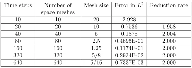
convergence rate. Table 2 shows that the choice of 15z-points in the contour with the proposed method is enough to obtain the same level of tolerance attained using 640 time steps with the Crank-Nicolson method. Observe that for eachz-point the cost of solving the complex-valued elliptic problem using the proposed method is almost comparable to that of advancing one step forward by solving the real-valued elliptic problem with the time-marching algorithms.
In the proposed scheme, we need the value of κas in Lemma 3.7 to determine the location of a integration contour. Since the coefficients are constants, if we choose the asymptotic slope of the contour as 0.4, we haveκ= 0.01811 by (3.8), and therefore the contour has to cut the real line at a point greater than 0.01811. Under this constraint, we choose the optimal parameters which are suggested in [37], and these parameters are attached in Table 3 in the case that the evaluation time is 1.0 for different iteration numbers. In particular, Table 3 says that 12 iterations are enough to balance with the space discretization of 2560 spatial meshes.
Time steps Number of space meshes
Mesh size Error inL2 Reduction rate
10 10 20 2.928
20 20 10 0.7536 1.958
40 40 5 0.1878 2.004
80 80 2.5 0.4695E-01 2.000
160 160 1.25 0.1174E-01 2.000
320 320 5/8 0.2934E-02 2.000
[image:12.612.141.468.342.459.2]640 640 5/16 0.7337E-03 2.000
Table 1. Example 4.1 with the Crank-Nicolson method
Number ofz Number of space meshes
Mesh size Error inL2 Reduction rate
15 10 20 2.924
15 20 10 0.7524 1.959
15 40 5 0.1876 2.004
15 80 2.5 0.4688E-01 2.000
15 160 1.25 0.1172E-01 2.000
15 320 5/8 0.2930E-02 2.000
[image:12.612.137.473.511.623.2]15 640 5/16 0.7327E-03 2.000
Table 2. Example 4.1 with the Laplace transformation method
Example 4.2 (European put option with transparent boundary condition). We consider a European put option with coefficients r = 0.05, σ= 0.3, T = 1.0 and K= 50and we truncate the domain atL= 50.
Number of z
Number of space meshes
L2-Error Reduction
rate
γ ν s τ
[image:13.612.125.495.165.291.2]3 2560 0.6397E-00 13.48 12.42 0.4213 0.16500 6 2560 0.1705E-01 5.229 26.95 24.84 0.4213 0.09385 9 2560 0.3434E-03 5.634 40.43 37.26 0.4213 0.06809 12 2560 0.5642E-04 2.605 53.90 49.68 0.4213 0.05430 15 2560 0.4731E-04 0.003 67.38 62.09 0.4213 0.04556 18 2560 0.4721E-04 0.001 80.86 74.51 0.4213 0.03947 21 2560 0.4717E-04 0.000 94.33 86.93 0.4213 0.03494
Table 3. Contour Parameters for Example 4.1
however, gives second order convergence which is shown in Table 2 although its domain is much smaller than that for Example 4.1. Indeed, comparing the same mesh sizes in Table 5 and Table 2, one can observe the numerical values are almost identical. In Figure 1 we can see the difference between the transparent boundary condition and the Dirichlet boundary.
Number ofz Number of space meshes
Mesh size Error inL2 Reduction rate
15 10 5 10.35
15 20 2.5 10.40 -0.007
15 40 1.25 10.41 -0.002
15 80 5/8 10.42 0.000
15 160 5/16 10.42 0.000
15 320 5/32 10.42 0.000
[image:13.612.139.473.418.532.2]15 640 5/64 10.42 0.000
Table 4. Example 4.2 with the Dirichlet boundary condition at
L= 50
Number ofz Number of space meshes
Mesh size Error inL2 Reduction rate
15 10 5 0.1870
15 20 2.5 0.4656E-01 2.006
15 40 1.25 0.1163E-01 2.001
15 80 5/8 0.2907E-02 2.000
15 160 5/16 0.7267E-03 2.000
15 320 5/32 0.1817E-03 1.999
15 640 5/64 0.4551E-04 1.998
Table 5. Example 4.2 with the transparent boundary condition
[image:13.612.139.472.599.715.2]0 5 10 15 20 25 30 35 40 45 50
0 10 20 30 40 50
Option Value
Stock Price dirichlet bd.
[image:14.612.163.441.151.365.2]transparent bd. exact sol.
Figure 1. Comparison between the Dirichlet boundary condition
and the transparent boundary condition (3.14) in Example 4.2
Example 4.3(Basket option with two underlying assets). We consider a European put basket option with two underlying assets having coefficientsr= 0.05,a11= 0.09, a22 = 0.09, a12 =a21 = −0.018, time to maturity=1.0, artificial boundary L1 =
300, L2= 300 and payoff function(100−max(x1, x2))+ is given.
For numerical computation, the boundary conditions are given by
∂u
∂ν(x, t) = 0, for (x, t)∈ {0} ×(0, L2)∪(0, L1)× {0}
×(0, T],
u(x, t) = 0, for (x, t)∈ {L1} ×(0, L2)∪(0, L1)× {L2}
×(0, T].
(4.2)
To evaluate the convergence rates for the proposed scheme, we solve the same problem using the Crank-Nicolson scheme on a 512×512 space grid for the extended artificial domain L1 = L2 = 600 with ∆t = 0.02. We set this as the reference
solution and calculate the relativeL2error for the proposed scheme. The integration
contour is built using the parametersγ= 35.94, ν= 33.12, s= 0.4213, τ = 0.07472. Numerical results in Table 6 show an almost second-order convergence rate.
Number ofz Number of space meshes
Mesh size Relative error inL2
Reduction rate
15 16×16 75/4 0.3662E-01
15 32×32 75/8 0.1047E-01 1.806
15 64×64 75/16 0.2969E-02 1.819
15 128×128 75/32 0.8444E-03 1.814
Table 6. Convergence rate in Example 4.3 on the domain
[0,300]×[0,300]
boundary condition (4.2) is replaced with
∂bu ∂x1
(L1, x2, z) =
1
L1a11 (
−(r−1 2a11)−
+
r r−1
2a11
2
+ 2a11(r+z) )
b
u(L1, x2, z)
on (x1, x2, z)∈ {L1} ×(0, L2)×Γ, and
∂bu
∂x2(x1, L2, z) =
1
L2a22 (
−(r−12a22)− + r
r−12a222+ 2a22(r+z) )
b
u(x, L2, z)
on (x1, x2, z) ∈(0, L1)× {L2} ×Γ. In Table 7 we compare the results produced
by the different boundary conditions on the lines L1 = 150 and L2 = 150. As
can be seen in Table 7, the transparent boundary condition is more accurate than the Dirichlet boundary condition. Furthermore, Table 6 and Table 7 show that if we apply the transparent boundary condition, it gives competitive error level in comparison to the Dirichlet boundary condition even though its computational domain is a quarter size of that with the Dirichlet boundary conditions applied.
Num-ber of
z
Number of space meshes
Mesh size Relative error in
L2(Dirichlet)
Relative error in
L2(Transparent)
[image:15.612.127.489.175.285.2]15 16×16 75/8 0.1998E-01 0.1076E-01 15 32×32 75/16 0.1176E-01 0.3485E-02 15 64×64 75/32 0.9283E-02 0.1724E-02
Table 7. Effect of boundary conditions in Example 4.3 on the
domain [0,150]×[0,150]
Since the elliptic equations in (3.1) forz=zk, k= 0,1,2,· · ·, N,are independent
each other, no communication is required during the computation except for the last summation step in the numerical Laplace inversion. Thus the Laplace transfor-mation method is very well fitted for parallel computation. The result in Table 8 is generated on 128×128 space grid forL1=L2= 300 with a 15-number ofzpoints
using IBM PowerPC97 with 2.2GHz clock speed. This table, as can be expected, shows almost ideal speedup because of the minimization of communication time. Finally, we attach the plot of the basket option price at Figure 2.
Number of CPUs 1 3 5 15
Time(sec) 74.93 25.25 15.31 5.671 Speedup 1.00 2.97 4.89 13.2
Table 8. Parallelization speedup in Example 4.3
References
[1] Y. Achdou and O. Pironneau.Computational methods for option pricing. SIAM, Philadel-phia, 2005.
[2] T. J. I’a. Bromwich. Normal coordinates in dynamical systems. Proc. Lond. Math. Soc., 15(Ser. 2):401–448, 1916.
[3] A. M. Cohen.Numerical methods for Laplace transform inversion. Springer, New York, 2007. [4] M. Crouzeix, S. Larsson, and V. Thom´ee. Resolvent estimates for elliptic finite element
[image:15.612.196.414.600.638.2]0 30
60 90
120
150 0 30
60 90
120 150 0
20 40 60 80 100
Price of Basket Option At Time 1.0
Stock 1 Price
[image:16.612.176.455.217.360.2]Stock 2 Price -10 0 10 20 30 40 50 60 70 80 90 100
Figure 2. Basket option price of Example 4.3
[5] K. S. Crump. Numerical inversion of Laplace transforms using a Fourier series approximation.
J. ACM, 23(1):89–96, 1976.
[6] D. I. Cruz-B´aez and J. M. Gonz´alez-Rodriguez. A different approach for pricing European options. InMATH’05: Proceedings of the 8th WSEAS International Conference on Applied Mathematics, pages 373–378, Stevens Point, Wisconsin, USA, 2005. World Scientific and Engineering Academy and Society (WSEAS).
[7] M. C. Fu, D. B. Madan, and T. Wang. Pricing continuous Asian options: a comparison of Monte Carlo and Laplace transform inversion methods.Journal of Computational Finance, 2:49–74, 1998.
[8] I. P. Gavrilyuk, , W. Hackbusch, and B. N. Khoromskij.H-matrix approximation for the operator exponential with applications.Numer. Math., 92:83–111, 2002.
[9] I. P. Gavrilyuk, W. Hackbusch, and B. N. Khoromskij. Data-sparse approximation to a class of operator-valued functions.Math. Comp., 74(250):681–708 (electronic), 2005.
[10] P. Glasserman.Monte Carlo Methods in Financial Engineering. Springer, 2003.
[11] M. Griebel. A domain decomposition method using sparse grids. InDomain Decomposition Methods in Science and Engineering: The Sixth International Conference on Domain De-composition, volume 157 ofContemporary Mathematics, pages 255–261, Providence, Rhode Island, 1994. American Mathematical Society.
[12] R. Kangro and R. Nicolaides. Far field boundary conditions for Black-Scholes equations.
SIAM J. Numer. Anal., 38:1357–1368, 2000.
[13] J. Lee and D. Sheen. An accurate numerical inversion of Laplace transforms based on the location of their poles.Comput & Math. Applic., 48(10–11):1415–1423, 2004
[14] J. Lee and D. Sheen. A parallel method for backward parabolic problems based on the Laplace transformation.SIAM J. Numer. Anal., 44:1466–1486, 2006.
[15] C. C. W. Leentvaar and C. W. Oosterlee. Pricing multi-asset options with sparse grids and fourth order finite differences. InNumerical mathematics and advanced applications, pages 975–983. Springer, Berlin, 2006.
[16] C.C.W. Leentvaar and C.W. Oosterlee. On coordinate transformation and grid stretching for sparse grid pricing of basket options.J. Comput. Appl. Math., 222(1):193–209, 2008. [17] M. L´opez-Fern´andez and C. Palencia. On the numerical inversion of the laplace transform of
certain holomorphic mappings.Appl. Numer. Math., 51:289–303, 2004.
[19] A.-M. Matache, C. Schwab, and T. P. Wihler. Fast numerical solution of parabolic inte-grodifferential equations with applications in finance.SIAM J. Sci. Comput., 27(2):369–393 (electronic), 2005.
[20] A.-M. Matache, T. von Petersdorff, and C. Schwab. Fast deterministic pricing of options on L´evy driven assets.M2AN Math. Model. Numer. Anal., 38(1):37–71, 2004.
[21] W. McLean, I. H. Sloan, and V. Thom´ee. Time discretization via Laplace transformation of an integro-differential equation of parabolic type.Numer. Math., 102:497–522, 2006. [22] W. McLean and V. Thom´ee. Time discretization of an evolution equation with Laplace
trans-forms.IMA J. Numer. Anal., 24:439–463, 2004.
[23] A. Murli and M. Rizzardi. Algorithm 682: Talbot’s method for the Laplace inversion problem.
ACM Trans. Math. Software, 16:158–168, 1990.
[24] R. Panini and R. P. Srivastav. Pricing perpetual options using Mellin transforms.Appl. Math. Lett., 18:471–474, April 2005.
[25] A. Pelsser. Pricing double barrier options using Laplace transforms.Finance and Stochastics, 4(1):95–104, 2000.
[26] W. H. Press, S. A. Teukolsky, W. T. Vetterling, and B. P. Flannery. Numerical recipes in Fortran 90, volume 2 ofFortran Numerical Recipes. Cambridge University Press, Cambridge, second edition, 1996.
[27] C. Reisinger and G. Wittum. Efficient hierarchical approximation of high-dimensional option pricing problems.SIAM J. Sci. Comput., 29(1):440–458 (electronic), 2007.
[28] R. U. Seydel.Tools for Computational Finance. Springer, second edition, 2003.
[29] D. Sheen, I. H. Sloan, and V. Thom´ee. A parallel method for time-discretization of par-abolic problems based on contour integral representation and quadrature. Math. Comp., 69(229):177–195, 2000.
[30] D. Sheen, I. H. Sloan, and V. Thom´ee. A parallel method for time-discretization of parabolic equations based on Laplace transformation and quadrature.IMA J. Numer. Anal., 23(2):269– 299, 2003.
[31] A. Talbot. The accurate numerical inversion of Laplace transforms.J. Inst. Maths. Applics., 23:97–120, 1979.
[32] D. Tavella and C. Randall.Pricing Financial Instruments: The Finite Difference Method. Wiley, 2000.
[33] V. Thom´ee. A high order parallel method for time discretization of parabolic type equations based on Laplace transformation and quadrature.Int. J. Numer. Anal. Model., 2:121–139, 2005.
[34] T. von Petersdorff and C. Schwab. Numerical solution of parabolic equations in high dimen-sions.M2AN Math. Model. Numer. Anal., 38(1):93–127, 2004.
[35] W. T. Weeks. Numerical inversion of Laplace transforms using Laguerre functions.J. ACM, 13(3):419–429, 1966.
[36] J. A. C. Weideman. Algorithms for parameter selection in the Weeks method for inverting Laplace transforms.SIAM J. Sci. Comput., 21(1):111–128, 1999.
[37] J. A. C. Weideman and L. N. Trefethen. Prabolic and hyperbolic contours for computing the Bromwich integral.Math. Comp., 76(259):1341–1356, Mar 2007.
[38] D. V. Widder.The Laplace transform. Princeton University Press, Princeton, N.J., 1941.
Interdisciplinary Program in Computational Science & Technology, Seoul National University, Seoul 151–747, Korea
E-mail:hyoseop2@snu.ac.kr
URL:http://www.nasc.snu.ac.kr/hslee/
Department of Mathematics, and Interdisciplinary Program in Computational Science & Tech-nology, Seoul National University, Seoul 151–747, Korea
E-mail:sheen@snu.ac.kr


![Table 7. Effect of boundary conditions in Example 4.3 on thedomain [0, 150] × [0, 150]](https://thumb-us.123doks.com/thumbv2/123dok_us/8129230.241730/15.612.196.414.600.638/table-eect-boundary-conditions-example-thedomain.webp)

