Methods to retrieve the complex refractive index of aquatic suspended particles: going beyond simple shapes

www.biogeosciences.net/13/4081/2016/ doi:10.5194/bg-13-4081-2016

© Author(s) 2016. CC Attribution 3.0 License.

Methods to retrieve the complex refractive index of aquatic

suspended particles: going beyond simple shapes

Albert-Miquel Sánchez and Jaume Piera

Institute of Marine Sciences (ICM-CSIC), Physical and Technological Oceanography Department, Pg. Marítim de la Barceloneta, 37-49, 08003, Barcelona, Spain

Correspondence to:A.-M. Sánchez ([email protected])

Received: 9 October 2015 – Published in Biogeosciences Discuss.: 24 November 2015 Revised: 3 July 2016 – Accepted: 4 July 2016 – Published: 18 July 2016

Abstract. The scattering properties of aquatic suspended particles have many optical applications. Several data inver-sion methods have been proposed to estimate important fea-tures of particles, such as their size distribution or their re-fractive index. Most of the proposed methods are based on the Lorenz–Mie theory to solve Maxwell’s equations, where particles are considered homogeneous spheres. A generaliza-tion that allows considerageneraliza-tion of more complex-shaped parti-cles is theT-matrix method. Although this approach imposes some geometrical restrictions (particles must be rotationally symmetrical) it is applicable to many life forms of phyto-plankton. In this paper, three different scenarios are consid-ered in order to compare the performance of several inversion methods for retrieving refractive indices. The error associ-ated with each method is discussed and analyzed. The results suggest that inverse methods using the T-matrix approach are useful to accurately retrieve the refractive indices of par-ticles with complex shapes, such as for many phytoplankton organisms.

1 Introduction

Light particle interactions, usually wavelength dependent, cause observable optical phenomena (e.g., changes on the ocean color or light extinction with depth) that allow as-sessing the composition of small particles (e.g., phytoplank-ton, sediment, or microplastics) in the water column (Mob-ley, 1994; Kirk, 1994). Understanding the interaction of light with particles is the central topic of many bio-optical studies where the water particle composition is inferred from in situ

or remote-sensing optical observations (Gordon and Morel, 2012, and references therein).

Maxwell’s equations are the basis of theoretical and com-putational methods describing light interaction with parti-cles. However, exact solutions to Maxwell’s equations are only known for selected geometries. Scattering from any ho-mogeneous spherical particle of arbitrary size is explained analytically by the Lorenz–Mie (also known as Mie) the-ory (Lorenz, 1898; Mie, 1908). Although bio-optical models usually assume that particles are spheres, most particles that contribute significantly to light interactions are indeed non-spherical, with aspect ratios (ratio of the principal axes of a particle) spanning between 0.4 and 72 (Clavano et al., 2007, and references therein). For more complex-shaped particles, scattering can be computed using theT-Matrix theory (Wa-terman, 1965), currently the fastest exact technique for the computation of nonspherical scattering based on a direct so-lution of Maxwell’s equations (Mischenko et al., 1996). The T-matrix method has some geometrical restrictions, such as axial symmetry, but it is applicable to many life forms of phy-toplankton and suspended mineral particles (Quirantes and Bernard, 2004; Sun et al., 2016), as shown in Fig. 1.

(a) Lorenz-Mie

(b) T-Matrix Stephanopyxis

(diatom)

Pediastrum (chlorophyceae) Coscinodiscus

(diatom)

Pennate diatom

Figure 1. (a)The Lorenz–Mie method only describes the scattering of an electromagnetic plane wave by a homogeneous sphere, while

(b)theT-Matrix method also characterizes the scattering by non-spherical particles such as spheroids, cylinders, or Chebyshev par-ticles. Both can be used on actual phytoplankton particles by using a suitable shape.

Several inverse models to retrieve the refractive index from optical measurements can be found in the literature. For in-stance, a single equation based on the Lorenz–Mie theory was used by Twardowski et al. (2001) to estimate the real part of the refractive index of a bulk oceanic distribution. It is indeed a fast method if optical backscattering measurements are available. Stramski et al. (1988) presented an extension of a model from Bricaud and Morel (1986), designed for iso-lated phytoplankton cultures (or dominated by one particular phytoplankton species). It is based on the anomalous diffrac-tion approximadiffrac-tion (ADA), which allows computing the real and imaginary parts of the complex refractive index as sepa-rate variables, using only the absorption and attenuation effi-ciency factors and the concurrent measurement of the particle size distribution (PSD). Bernard et al. (2001) simplified this model by replacing the Lorentzian oscillators with a simple Hilbert transform. All these methods share one thing in com-mon: they approximate the shape of the particles by homo-geneous spheres. First Meyer (1979) and later Bernard et al. (2009) suggested that two-layered spherical geometry mod-els reproduce the measured algal angular scattering proper-ties more accurately. Finally, a combination of a genetic al-gorithm with the Lorenz–Mie andT-Matrix approaches was used by Sánchez et al. (2014), thereby allowing the study of more complex structures than simple homogeneous or coated spheres. A genetic algorithm is a method to solve problems simulating the process of natural selection using inheritance, mutation, selection, and crossover between different possible solutions. This method only requires the measured attenua-tion and scattering coefficients, together with the PSD, to find

the complex refractive index. It is much slower than the pre-vious ones (in particular, for nonspherical particles), but it can provide very accurate estimations.

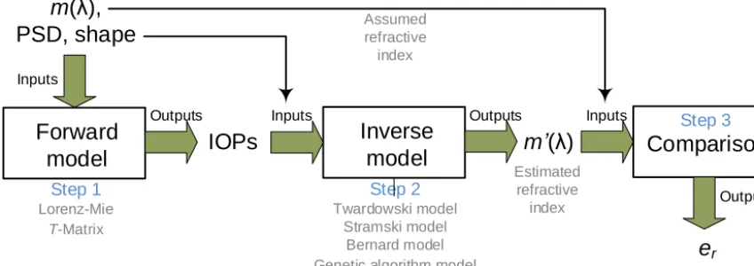
In this paper, the above refractive index retrieval mod-els are reviewed and tested against simulated data in order to analyze their accuracy when modeling real (and usually complex-shaped) particles suspended in water, such as phy-toplankton. The comparison has been done following the three steps presented in Fig. 2. First, the forward models (basically, Lorenz–Mie andT-Matrix methods) are used to obtain the inherent optical properties (IOPs) of a selected configuration using as inputs the postulated wavelength-dependent refractive index,m(λ), the PSD, and the particle shape. Second, the above inverse models are used to estimate the refractive index from the IOPs along with the PSD and the particle shape. Finally, the estimated refractive index is compared with the postulated one in order to assess the ac-curacy of the inverse model.

The simulated examples are implemented using complex refractive indices and PSDs similar to those found in nature for phytoplankton species. Since phytoplankton particles ex-hibit a wide variety of shapes, each example has been pro-vided with a different outline accounting for a homogeneous sphere, a coated sphere, and a homogeneous cylinder. None of these idealized shapes is an exact representation of real al-gae presenting cell walls, chloroplasts, vacuoles, nuclei, and other internal organelles, each one with its own optical prop-erties. However, they can be considered as a first approxima-tion suitable for the purposes of the tests presented in this contribution.

It must also be noted that the models are fundamentally different. The model developed by Twardowski et al. (2001) is intended to be used for entire particle populations that are assumed to follow a power-law size distribution, whereas the other models are developed for single phytoplankton cultures (or dominated by one particular phytoplankton species) and require the concurrent measurement of the size distribution. These bio-optical models are also compared with a numer-ical method (i.e., the genetic algorithm) in the same condi-tions. On the other hand, our approach allows an objective comparison of the results from the different methods in those occasions when no single optimum methodology is clearly identifiable, a tool of potentially high interest for the ocean optics community.

Forward

model

m

(λ),

PSD, shape

IOPs

Inverse

model

m

(λ)

Comparison

Inputs

Outputs Inputs Outputs Inputs

Outputs

e

Step 1 Lorenz-Mie

T-Matrix

Step 2 Twardowski model

Stramski model Bernard model Genetic algorithm model

Assumed refractive

index

Estimated refractive

index

Relative error

Figure 2.Procedure used to analyze the accuracy of the inverse models.

2 Model theory

2.1 Size distributions and polydispersions

Algal assemblages are typically polydispersed with regard to size, and can be described by a PSDF (D), whereDis the particle diameter, andF (D)d(D)is the number of particles per unit volume in the size rangeD±1/2d(D)(Bricaud and Morel, 1986). Using absorption as an example (analogous expressions may be used for other IOPs, i.e., those related to light extinction and scattering), the absorption efficiency factor representing the mean of a size distribution can be de-scribed by (Bricaud and Morel, 1986):

Q_a(λ)=

R∞

0 Qa(λ, D)F (D)D2d(D) R∞

0 F (D)D2d(D)

, (1)

whereλis the wavelength. The total absorbed power per unit incident irradiance and unit volume of water, i.e., the absorp-tion coefficient, is then either given by

a(λ)=π

4 ∞

Z

0

Qa(λ, D)F (D)D2d(D) h

m−1i, (2)

or, using the result of Eq. (1), by

a(λ)=π

4Qa(λ) ∞

Z

0

F (D)D2d(D) hm−1i. (3)

2.2 Inherent optical properties

Lorenz–Mie andT-Matrix theories are powerful methods to formulate an analytical solution to electromagnetic scatter-ing by spherical and nonspherical particles. Both rely on the expansion of the incoming light into spherical harmonics and

use an intensive formulation to compute the coefficients that link the incident field with the scattered and transmitted ones. The complete Lorenz–Mie derivation is reviewed by Bohren and Huffman (1998), and theT-Matrix approach is described by Mischenko et al. (1996). Both theories provide the par-ticle specific optical properties, i.e., the extinction, scatter-ing, and absorption cross sections that describe the fraction of the incident beam intensity converted to extinct, scattered, or absorbed light,Ce,Cs, andCa, respectively, in terms of

ef-fective area. The relationship between wavelength-dependent efficiency factors and cross sections is

Qx(λ)=

Cx(λ)

hGi , (4)

withx being any of the subindicese,s, ora to denote ex-tinction, scattering, or absorption, andGthe geometric cross section of the particle (in the case of nonspherical particles,

hGiis the averaged cross-sectional area over all orientations). The cross sections obtained from the Lorenz–Mie and T -Matrix approaches (size averaged in polydisperse concentra-tions as described above) can also be used to compute the extinction, scattering, and absorption coefficients (c(λ),b(λ), anda(λ), respectively) (Quirantes and Bernard, 2006) as

c(λ)=N· hCe(λ)i h

m−1i, (5)

b(λ)=N· hCs(λ)i h

m−1i, (6)

a(λ)=N· hCa(λ)i h

m−1i, (7)

whereN denotes the number of particles per unit volume. The relationship between the three parameters is

Scattering can be further characterized in terms of the an-gular distribution of the scattered light using the volume scat-tering function (β) (Mobley, 1994) as

β(9, λ)=β(9, λ)e ·b(λ) h

m−1m−1i, (9) where9 is the scattering angle, i.e., the angle between the incident and scattered beams, and β(9, λ)e is the scattering

phase function and the (1,1)element of the Stokes scatter-ing matrix (or Mueller matrix). This matrix, obtained with the Lorenz–Mie andT-Matrix formulation when the physi-cal characteristics of the particles are known, transforms the Stokes parameters of the incident light into those of the scat-tered light. By integrating the volume scattering function in all directions, assuming azimuthal symmetry, the total scat-tering coefficientbis obtained as

b(λ)=2π

π Z

0

β(9, λ)sin(9)d9 hm−1i, (10)

which can be partitioned into its forward and backward com-ponents (respectively,bf andbb) by limiting the integration

limits from 0 toπ/2 and from π/2 to π, respectively. The backscatter fraction, defined by

Bb(λ)=

bb(λ)

b(λ), (11)

gives the fraction of scattered light that is deflected through the scattering angles above π/2. Given Eqs. (9) and (10), the normalization condition for the volume scattering phase function is

2π

π Z

0 e

β(9, λ)sin(9)d9=1. (12)

This normalization implies that the backscatter fraction can be computed using the volume scattering phase function as

Bb(9, λ)=2π π Z

π

2 e

β(9, λ)sin(9)d9. (13)

The 2πfactor used in Eqs. (10), (12), and (13) arises natu-rally after integration with respect to the azimuth angle. No-tice that the same 2πfactor is also used by Twardowski et al. (2001), Bohren and Huffman (1998), and in most of the lit-erature on ocean optics (Mobley, 1994), but differs from the one-half factor used by Mischenko et al. (1996), Mischenko and Travis (1998), Wiscombe and Grams (1976), and Mug-nai and Wiscombe (1986), where the integration of phase function is normalized to 4π, representing the total solid an-gle over the whole sphere.

3 Review of refractive index retrieval models

In this section, a review of the different approximations to re-trieve the refractive index (inverse models) is presented. Each model is named after the lead author of the publication. The complex refractive indexm (λ)is defined as

m (λ)=n (λ)+ik (λ) , (14)

where the real partn (λ)determines the phase velocity of the propagating wave, and the imaginary partk (λ)determines the flux decay. The sign of the complex part is a matter of convention as it may also be defined with a negative sign. The above notation corresponds to waves with time evolu-tion given bye−iωt. Notice that, throughout this paper, the effective refractive indices are computed relative to seawater, which has a constant value ofmwater=1.334+i0 (this value varies with wavelength, salinity, temperature, and pressure, Hale and Querry, 1973). Thus, values relative to free vacuum can be obtained byma=m×mwater.

3.1 The Twardowski model

The Twardowski model (Twardowski et al., 2001) is based on Volz (1954) as cited in van de Hulst (1957). It is derived using the Lorenz–Mie theory and the relationship between the particulate spectral attenuation (cP(λ)) and the size

dis-tribution to retrieve the bulk particulate refractive index from in situ optical measurements. In particular, it assumes that γ=ξ−3 (γ is the hyperbolic slope of the attenuation co-efficient andξ is the power-law slope of the PSD). It only considers power-law distributions that fulfill the conditions 2.5≤ξ≤4.5 and 0≤Bb≤0.03. The bulk refractive index

is obtained from a polynomial fit to the Lorenz–Mie calcula-tions:

ˆ

n (Bb, γ )=1+B0.5377

+0.4867γ2 b

1.4676+2.2950γ2+2.3113γ4

. (15)

later taken into account by Boss et al. (2004), but without re-computing the regression. This means that some inaccuracies can be expected when using ideal models.

3.2 The Stramski model

This model is based on the methods presented by Stramski et al. (1988), which are an extension of those developed by Bricaud and Morel (1986). It is based on the ADA, first de-scribed in van de Hulst (1957). The ADA offers approxima-tions to the absorption and attenuation optical efficiency fac-tors using relatively simple algebraic formulae, based on the assumptions that the particle is large relative to the wave-length (α=π D

λ 1) and that the refractive index is small

(n−11 andk1). This method allows decoupling the effects of the real and imaginary refractive indices on absorp-tion and scattering. Assuming a homogeneous geometry, the ADA expression for the absorption efficiency factor is given by

Qa ρ0=1+

2e−ρ0 ρ0 +2

e−ρ0−1

ρ02 , (16)

where ρ0=4αk is the absorption optical thickness. Equa-tions (3) and (16) are then used iteratively to determine the homogeneous imaginary part of the refractive index (k(λ)) in conjunction with measured algal absorption and PSD data. According to the Ketteler–Helmholtz theory of anomalous dispersion (van de Hulst, 1957), a variation inkinduces vari-ations inn, quantified with a series of oscillators (represent-ing discrete absorption bands) based on the Lorentz–Lorenz equations (Stramski et al., 1988; Bricaud and Morel, 1986). These spectral variations (denoted as1n(λ)) vary around a central value of the real refractive index, 1+. Thus,

n(λ)=1++1n(λ). (17)

The central value 1+is estimated by computing the non-absorbent equivalent population attenuation efficiency factor (QNAE_c ) at those wavelengths where1n(λ)=0.

Consider-ing polydispersion, this is done accordConsider-ing to

QNAE_c (ρ)=

R∞

0 Qc(ρ)F (ρ)ρ 2_d(ρ)

R∞

0 F (ρ)ρ2d(ρ)

, (18)

whereρ=2α(n−1), andF (ρ)is obtained from the exper-imental size distribution by replacingD byρ, and calculat-ingQc(ρ)with the van de Hulst’s formula assumingξ=0

(van de Hulst, 1957):

Qc(ρ)=2−

4 ρsinρ+

4

ρ2(1−cosρ). (19)

The exact value ofis indicated by a value ofQNAE_c (ρ) that is equal toQc(λ).

This methodology was subsequently simplified by Bernard et al. (2001, 2009) using the Kramers–Kronig relations, in-stead of employing the Lorentzian oscillators, to compute the spectral variations in the real part of the refractive index on the basis of the imaginary part. The Kramers–Kronig rela-tions describe the mutual dependence of the real and imagi-nary parts of the refractive index through dispersion, as does the Ketteler–Helmholtz theory, but they are simpler than the tedious and sometimes inaccurate use of summed oscillators (the real part is the Hilbert transform of the imaginary part; van de Hulst, 1957).

3.3 The Bernard model

Meyer (1979) and Bernard et al. (2009) suggested that two-layered spherical geometry models reproduce the mea-sured algal angular scattering properties more accurately. For Bernard et al. (2009), the outer layer accounts for the chloro-plast and the inner layer for the cytoplasm. Refractive index values are assumed for the cytoplasm, with a spectral imagi-nary part modeled as

kcyto(λ)=kcyto(400)e[−0.01(λ−400)], (20) wherekcyto(400)=0.0005. The real refractive index spec-tra for the cytoplasm,ncyto(λ), are obtained using the Hilbert transform (absorption has an influence on scattering and at-tenuation, expressed through the Kramers–Kronig relations) and Eq. (17) with 1+=1.02. Usingkcyto(λ)from Eq. (20), the volume equivalent values ofkchlor(λ)is determined using the Gladstone–Dale formulation:

kchlor(λ)=

kh(λ)−kcyto(λ)VV

1−VV

, (21)

wherekh(λ)is the imaginary part of the refractive index

con-sidering homogeneous cells and obtained using Eq. (16), and VV is the relative chloroplast volume. According to Bernard

et al. (2009), a VV value of 20 % can be considered as a

first approximation for a spherical algal geometry, although higher values should be considered for the large-celled di-noflagellate and cryptophyte samples. Other studies have employed relative chloroplast volumes ofVV =41 %

(Zan-eveld and Kitchen, 1995),VV =58 % (Latimer, 1984), and

VV =27 to 66 % (Bricaud et al., 1992). The real refractive

index spectra for the chloroplastnchlor(λ) is then generated by a Hilbert transform and using Eq. (17) with 1+values between 1.044 and 1.14, depending on the sample.

3.4 The genetic algorithm model

when using the Lorenz–Mie or T-Matrix approaches with the measured PSD. The methodology of the algorithm may be summarized as follows (Fig. 3). First, a random vector of solutions is generated for a specific wavelength ([m1(λi),

m2(λi),. . ., mn(λi)], whereλi denotes the selected

wave-length andm1, m2, . . ., mnthe complex refractive indices); if

possible, the search space is bound in order to maximize the algorithm success. Next, the complete vector is evaluated by the fitness function. This is done by computing thea(λ)and b(λ)coefficients corresponding to each refractive index (us-ing the Lorenz–Mie orT-Matrix formulation and Eqs. 6–7) and evaluating the weighted Euclidean distance between the calculated and desired coefficients. This can be done, for in-stance, as

ea(λi)= |20 log(aˆk(λi))−20 log(am(λi))|, (22)

where ak is the calculated absorption coefficient of the nk

refractive index,amis the desired (or measured) attenuation

coefficient, andeais the error in the absorption coefficient.

The use of logarithmic weighting improves the performance when dealing with small errors over small coefficients. The same equation can be applied for the scattering coefficient. Both results are finally combined using a quadratic mean, thus obtaining a single evaluation value that is minimized by the algorithm.

After the evaluation, the algorithm stops if a satisfactory fitness level or a maximum number of generations is reached (each generation is a new vector of solutions). If the con-vergence condition is not fulfilled, the best solutions are se-lected and taken apart. Part of this elite is then recombined (crossover) and randomly mutated to provide genetic diver-sity and broaden the search space (crossover and mutation introduce the diversity needed to ensure that the entire sam-ple space is reachable and suboptimal solutions are avoided; Greenhalgh and Marshall, 2000). The new set of solutions is re-evaluated and inserted again into the solutions’ vector, which completes the cycle. After converging, the algorithm presents the best possible solution.

Since the Lorenz–Mie andT-Matrix algorithms can only be executed for single wavelengths and the refractive index is also wavelength dependent, with different values at differ-ent wavelengths, the genetic algorithm completes the search procedure at a single wavelength each time. After each con-vergence, the process starts over with the next wavelength-dependent value, eventually obtaining the complete complex refractive index signature.

The main advantage of this method is that it can be easily adapted to different Lorenz–Mie orT-Matrix codes, for in-stance, as those developed for homogeneous spheres, coated spheres, and cylinders. Besides, it can also be easily com-bined with other models to improve the results. However, it should be noted that some inversions may be ill posed. A constrained optimization problem is considered to be well posed (in the sense of Hadamard) if (a) a solution exists,

(b) the solution is unique, and (c) the solution is well be-haved, i.e., varies continuously with the problem parameters. An ill-posed problem fails to satisfy one or more of these cri-teria (Bhandarkar et al., 1994); in this case, techniques such as regularization methods can be applied to improve the re-sults (Mera et al., 2004).

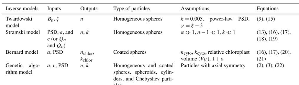
3.5 Summary of the refractive index retrieval models This section has been summarized in Table 1, showing, for each model, its inputs and outputs, type of particles, as well as the assumptions of the model and the equations used.

4 Simulations

The models described in the previous section are used here to retrieve the refractive index of well-known particles in order to determine their accuracy by means of the averaged relative error defined as

erx(%)=

1 N

N X

n=1

x0(λn)

x(λn)

−1

×100, (23)

wherex0is either the real part of the refractive index, esti-mated asn0(λ)−1 (the unity is subtracted to only consider the decimals), or the estimated imaginary part of the refrac-tive index,k0(λ), andxaccounts for the postulated real part of the refractive index,n(λ)−1, or the postulated imaginary part of the refractive index,k(λ). For the volume scattering function, the error is also averaged with respect to its angular contribution as

erVSF(%)= 1 N·M

N X n=1 M X m=1

V SF0_{(λn, θm)} V SF (λn, θm) −1

×100. (24)

Fitness

(a,b)=f(m) Conv.? Solution

Mutation Crossover Selection First

population

No

Yes Next

wavelength (λ)

Inputs: a(λ), b(λ), PSD

Fitness (a,b)=f(n)

Conv.?

Solution

Mutation

Crossover

Selection First

population

No

Ye

s

N

e

xt

w

a

ve

le

n

g

th

(

λ

)

Inputs: a(λ), b(λ), PSD

Figure 3.Flow chart for the genetic algorithm.

Table 1.Summary of the refractive index retrieval models.

Inverse models Inputs Outputs Type of particles Assumptions Equations

Twardowski model

Bb,ξ n Homogeneous spheres k=0.005, power-law PSD,

γ=ξ−3

(9), (15)

Stramski model PSD,a, and c(orQa

andQc)

n,k Homogeneous spheres α1,n−11,k1 (13), (16), (17), (18), (19)

Bernard model a, PSD nchlor, kchlor

Coated spheres ncyto,kcyto, relative chloroplast volume (VV), 1+

(16), (17), (20), (21)

Genetic algo-rithm model

a,c, PSD n,k Homogeneous and coated spheres, spheroids, cylin-ders, and Chebyshev parti-cles

Particles with axial symmetry (2), (3), (22)

phytoplankton, e.g., the diatom Thalassiosira pseudonana. Although this particle design does not exactly lead to the same optical behavior as the actual phytoplankton particle (the micro details of the cells are neglected) it can serve as a first approximation. The refractive indices are estimated from the combination of the genetic algorithm with the Bernard model for coated spheres and from the genetic algorithm alone.

4.1 Spherical-shaped homogeneous particles

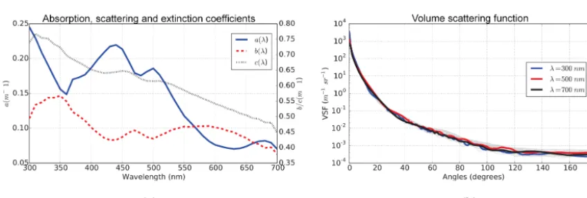
A concentration of 100 spherical particles per cubic millime-ter, with the PSD shown in Fig. 4a and the complex refrac-tive index of Fig. 4b), was simulated using the Lorenz–Mie scattering theory (Bohren and Huffman, 1998). This PSD is based on a power-law distribution (or Junge type) with 51 points,Rmin=0.7 µm,Rmax=12.1 µm, a slope parame-terξ=3, effective radiusreff=4 µm, and effective variance veff=0.6. In particular, the BHMIE code, originally from Bohren and Huffman (Bohren and Huffman, 1998) and mod-ified by B.T. Draine, was used as a forward model (additional features were added, such as polydispersion and the compu-tation of the Stokes scattering matrix). The computed IOPs from this forward model, i.e., thea(λ),b(λ), andc(λ) coef-ficients, are shown in Fig. 5a. As may be observed, the con-centration was selected in order to obtain IOP coefficients similar to those measured by Twardowski et al. (2001) and

Stramski et al. (2001). The power-law distribution is used in our calculations for two main reasons. First, even though it is not a realistic distribution for single-phytoplankton species, it is a fairly good approximation to natural water composi-tion even for anomalous condicomposi-tions such as phytoplankton blooms, as there is always a strong background contribution to the PSD (Twardowski et al., 2001); and second, because it is the only distribution that can be used in the Twardowski model.

and accessory pigments; as expected, a similar shape is prop-agated to the absorption coefficient spectra, a(λ)(Fig. 5a). The volume scattering function is shown in Fig. 5b. As par-ticles are relatively large relative to the wavelength, the scat-tering is mainly focused in the forward direction (between 0 and 10◦) and smoothly decreases in the backward direction. 4.1.1 The Twardowski model

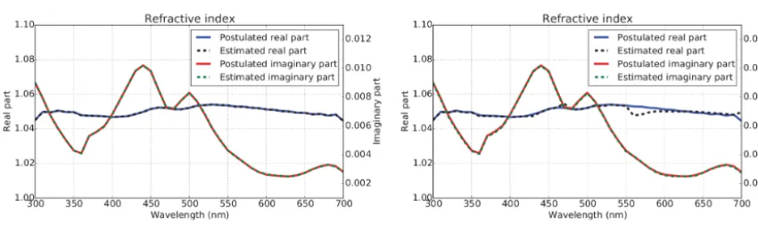
The spherical-shaped particle idealization was first examined with the Twardowski model. The use of Eq. (15) led to the re-sults shown in Fig. 6a;γ is set to 0, as the slope parameter of the PSD,ξ=3, and the backscatter fraction were computed with Eq. (13) using the volume scattering phase function val-ues given by the modified BHMIE code. For the real part, the model leads to a curve similar to the postulated complex re-fractive index, but with a slight negative offset, presenting an averaged relative error of 42 %. Since this model assumes a constant imaginary refractive index value of 0.005 (used for the development of the model), it has been considered as an output and compared with the postulated imaginary part of the refractive index, obtaining that the averaged relative error is 44 %. It should be noted that the Twardowski model was designed for a rather different scenario: a bulk oceanic dis-tribution presenting different physical properties than those of isolated species of phytoplankton, e.g., index of refraction and shape.

4.1.2 The Stramski model

This model overestimates both the real and imaginary parts for all analyzed spectra (Fig. 6b), showing an averaged rela-tive error of 0.4 % for the real part and a 15 % for the imagi-nary part. It should be remembered that the imagiimagi-nary part of the refractive index,kh, is calculated with the ADA, known

to give errors of about 10 % when compared with results from the Lorenz–Mie theory (Bernard et al., 2009). Some discrepancies can therefore be expected between the ADA and Aden–Kerker-derived values (Aden and Kerker, 1951). 4.1.3 The genetic algorithm model

In order to implement the genetic algorithm described in Sect. 3.4, the tools provided by the DEAP (Distributed Evo-lutionary Algorithms in Python) and SCOOP (Scalable COn-current Operations in Python) frameworks were used, re-spectively aimed at developing evolutionary algorithms and parallel task distribution (Fortin et al., 2012; Hold-Geoffroy et al., 2014). The fitness function was implemented using the fast subroutines of BHMIE to compute the absorption and scattering properties of homogeneous spheres. The co-efficients a(λ) andb(λ) of Fig. 5a were used as inputs to the genetic algorithm model in order to obtain the postulated complex refractive index, and limiting conditions were ap-plied to facilitate the convergence (typical values for the real part of the phytoplankton refractive indices fall between 1.02

and 1.15 relative to water, and the bulk value of the imagi-nary part is always below 0.02). The genetic algorithm was configured with a vector of 2000 solutions over 10 genera-tions and 50 and 20 % of probability of crossover and muta-tion, respectively, leading to the values shown in Fig. 7a. The good agreement between the postulated complex refractive index values and the estimated ones shows that it is possi-ble to perform accurate estimations with a genetic algorithm (averaged relative errors of 0.0 % for the real part and 0.2 % for the imaginary part represent the best results for spherical homogeneous particles). It should be noted that the number of generations necessary for a suitable convergence strongly depends on the length of the initial solution vector and the crossover and mutation percentages, among other parameters of the genetic algorithm. Adopting the previously described parameters, no significant improvement is generally found beyond the 10th generation.

One disadvantage of the genetic algorithms is that they are relatively slow and require more computation time than other optimization algorithms, as they compute the fitness func-tion many more times. Other optimizafunc-tion algorithms were also applied to determine whether similar results can be ob-tained with a significant reduction of the computation time. However, since none of them led to any meaningful improve-ment, no further description is provided. As a single exam-ple, Fig. 7b shows the results obtained with the much faster Broyden–Fletcher–Goldfarb–Shanno (BFGS) algorithm (an iterative method for solving unconstrained nonlinear opti-mization problems (Zhu et al., 1997)), executed using the same bounding conditions as in the genetic algorithm case. In this case, only 4 min were needed instead of 97 min when using the genetic algorithm. Both computations where performed using a PC with an Intel Core i7 processor at 3.2 GHz, with 16 GB of RAM. Although the BFGS results are generally satisfactory, some of the wavelengths present a significant error in the real part (mainly between 550 and 600 nm, and above 680 nm). The averaged relative error is 0.0 % for the real part and 0.7 % for the imaginary part. Other optimization algorithms, such as the conjugated gradi-ent algorithm (Nocedal and Wright, 1999), were also tested. The results (not shown) exhibited worse accuracy than the BFGS, indicating that the genetic algorithm is probably the best method to solve this problem (in terms of accuracy but not in terms of executing time).

4.2 Spherical-shaped coated particles

Figure 4. (a)PSD for the test run with spherical-shaped homogeneous particles.(b) Complex refractive index signature postulated for spherical-shaped homogeneous particles.

Figure 5. (a)Absorption (a(λ)), scattering (b(λ)), and extinction (c(λ)) coefficients and(b)the volume scattering function for spherical-shaped homogeneous particles (three wavelengths: 300, 500, and 700 nm, are plotted using intense colors, whereas the other wavelengths between 300 and 700 nm are plotted in light gray).

VV =30 %, a value that lies between those previously used

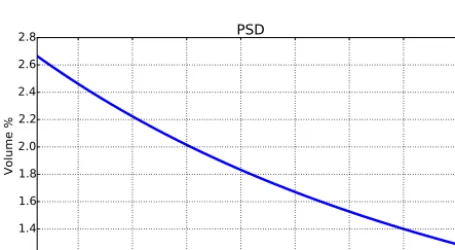
by Bernard et al. (2009) and other authors, and the real re-fractive index was calculated using the Hilbert transform and Eq. (17) with 1+=1.1. Figure 8a and b show the results for the real and imaginary parts, respectively (postulated val-ues). In this example, instead of using a PSD describing a power-law function as in Fig. 4a, the PSD of an isolated cul-ture was simulated with a concentration of 40 particles per cubic millimeter (Rmin=0.7 µm,Rmax=12.1 µm, and us-ing 31 points), as seen in Fig. 9. Notice that the PSD denotes the external radius while the inner one can be calculated us-ing theVV value. The absorption, scattering, and extinction

coefficients (Fig. 10a) and the volume scattering function (Fig. 10b) were obtained introducing these PSD and refrac-tive indices in the BART code of Quirantes (a forward model based on the Aden–Kerker theory to calculate light-scattering properties for coated spherical particles, Quirantes, 2005).

The above set of IOPs can now be used to estimate the corresponding complex refractive indices. First, the genetic algorithm is used in order to see whether a basic shape, such as a homogeneous sphere, is useful when modeling more complex particles. If coated particle models do

bet-ter at characbet-terizing the optical properties of general phyto-plankton species, as stated in Bernard et al. (2009), this can be used to estimate the error associated with using homoge-neous spheres. Next, the inner and outer complex refractive indices of the original particle are retrieved using the Bernard model for coated particles. Finally, a combination of the ge-netic algorithm and the Bernard model is applied to improve the previous results. Notice that the Twardowski model is not applied in order to avoid an inconsistent comparison with the other methods, as it was originally designed to be used with entire particle populations that are assumed to follow a power-law size distribution.

4.2.1 The genetic algorithm model

Figure 6.Postulated and estimated refractive indices using(a)the Twardowski and(b)the Stramski models.

Figure 7. (a)Postulated and estimated refractive indices using the genetic algorithm; notice that the postulated and estimated values lie on top of each other.(b)Postulated and estimated refractive indices using the BFGS algorithm.

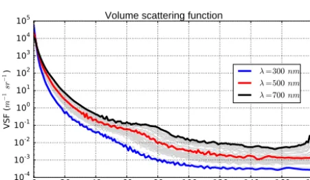
and similarly for the imaginary values (Fig. 8b). The volume scattering function for the homogeneous particles (Fig. 11) is obtained by means of the Lorenz–Mie (forward model), us-ing as inputs the estimated complex refractive index and the PSD (Fig. 9). This model presents similar values in the for-ward scattering but completely underestimates the backscat-tering, with values far below those in Fig. 10b. This example demonstrates that the common characterization using homo-geneous spheres is not a suitable methodology when deal-ing with complex particles. This is not a surprisdeal-ing result, as it has been discussed by Bohren and Huffman (1998), in the atmospheric context, and by Stramski et al. (2004), Cla-vano et al. (2007), Dall’Olmo et al. (2009), and Bernard et al. (2009), in the oceanic one, but the comparison between the two volume scattering functions highlights that the backscat-tering can exhibit errors of up to 1 order of magnitude. 4.2.2 The Bernard model

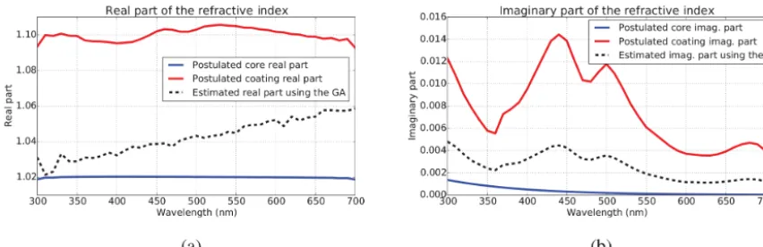
The Bernard model, described in Sect. 3.3, was used to es-timate the complex refractive index of the two-layered par-ticles. Figure 12a shows the postulated and estimated real part of the inner and outer layers and Fig. 12b shows the re-spective postulated and estimated imaginary parts. The in-ner refractive index is well estimated, an expected result as

the same equation is used for both generation and retrieval, but the outer refractive index is not in accurate agreement. In particular, the imaginary part is significantly underestimated, with an averaged relative error of 51 %. On the other hand, the simulation for the estimated refractive indices in coated spheres gives a volume scattering function that fits the pos-tulated values (Fig. 10b) better than the one produced by the homogeneous spherical particle (the volume scattering func-tion figure is not presented as the errors do not show up in the graph; a more detailed analysis is performed in Sect. 5 for this case).

4.2.3 The Bernard model combined with the genetic algorithm model

(ill-Figure 8.Postulated(a)real and(b)imaginary refractive index signatures for the inner and outer layers of spherical-shaped particles, together with the estimated(a)real and(b)imaginary refractive index signature calculated using the genetic algorithm model.

4 6 8 10 Radius [µm]

0 2 4 6 8 10

Volume %

PSD

Figure 9.PSD simulating an isolated culture.

posed) problem. Alternatively, the Bernard model could be combined with the genetic algorithm to increase the prob-ability of convergence. In this case, the inner refractive in-dex is again estimated using the Bernard model and the outer refractive index is then obtained with the genetic algorithm (coupled to the BART code). In this case, the genetic algo-rithm only has to find a solution with 2 degrees of freedom (the real and imaginary parts of the outer refractive index).

This method was applied to the coated particle example using the coefficients of Fig. 10a as input data and config-ured using an initial vector of 2000 solutions, 10 generations, 50 % of probability for crossovers, and 20 % for mutations. The postulated and estimated real parts of the inner and outer layers are shown in Fig. 13a and the corresponding postu-lated and estimated imaginary parts are presented in Fig. 13b. Accurate results were obtained, certainly improving the re-fractive index estimate for the outer sphere. In this particular case, average relative errors of 0.0 and 0.1 % were, respec-tively, obtained for the real and imaginary parts.

4.3 Cylindrical-shaped particles

As a final example, a cylindrical-shaped particle has been chosen. As commented above, phytoplankton species

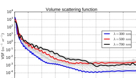
usu-ally present complex shapes, far from perfect homogeneous or coated spheres. This is the case, for example, of the cen-tric diatom with cylindrical shapes (to name a few genera: Thalassiosira, Aulacoseira, Skeletonema, Melosira, etc.). In order to find out the most accurate model for the charac-terization of such complex shapes, we considered an ex-ample consisting of 100 prolate cylinders per cubic mil-limeter with a diameter-to-length ratio equivalent to 0.8 and the PSD of Fig. 14 (showing the radius of an equivalent-volume sphere with slope parameterξ=3, effective radius reff=3.2 µm, and effective variance veff=0.005, resulting inRmin=0.8 µm toRmax=3.6 µm). The postulated refrac-tive index of Fig. 4b was simulated using theT-Matrix algo-rithm from M. Mischenko (Mischenko and Travis, 1998) for randomly oriented, rotationally symmetric scatterers (cylin-ders, spheroids, and Chebyshev particles). The PSD presents a small effective variance for convergence limitations of the code. The postulateda(λ), b(λ), and c(λ) coefficients are shown in Fig. 15a, and the volume scattering function at each wavelength is shown in Fig. 15b.

4.3.1 The Bernard model combined with the genetic algorithm model

As previously discussed, the simulated cylindrical particles are not exact duplicates of the actual phytoplankton organ-isms, so it is useful to compare the results using this and the coated sphere design (usually used on all kind of phy-toplankton shapes). As in previous examples, the postulated value ofVV for the coated sphere was 30 %, which is an

Figure 10. (a)Absorption (a(λ)), scattering (b(λ)), and extinction (c(λ)) coefficients and(b)volume scattering function for spherical-shaped coated particles.

0 20 40 60 80 100 120 140 160 180

Angles (degrees)

10-4

10-3

10-2

10-1

100

101

102

103

104

105

VS

F (

m

−

1sr

−

1)

Volume scattering function

λ=300 nm

λ=500 nm

λ=700 nm

Figure 11.Volume scattering function using the estimated refrac-tive index for spherical-shaped coated particles.

cylinders, are comparable. The volume scattering function is obtained (Fig. 17) by means of the estimated complex re-fractive indices and the PSD of Fig. 14 in a T-Matrix for-ward model. The error in this last figure is large, especially at long wavelengths, reaching an averaged relative error of 77 %. It should be noted that these differences may decrease when using real phytoplankton, since backscattering of het-erogeneous particles is different from that of homogeneous particles.

4.3.2 The genetic algorithm model

The genetic algorithm can be combined with the T -matrix code in order to consider cylindrical-shaped particles when estimating the inner complex refractive index. How-ever, when using the Mischenko code, one simulation of cylindrical-shaped particles needs about 67 min in a com-puter with an i7 processor at 3.20 GHz. This prevents us-ing the genetic algorithm, as an accurate estimate the com-plex refractive index would require executing this simula-tion several hundreds of times at each wavelength, or several months for the entire refractive index spectra. An alternative approach for obtaining fast estimates is to use spherical

ho-mogeneous particles with the same volume as the cylinders. This allows using the Lorenz–Mie theory rather than theT -matrix approach, dramatically reducing the simulation time. The refractive index estimated using the equal-volume ho-mogeneous spheres may then be applied for hoho-mogeneous cylinders in order to obtain their IOP, since the volume scat-tering function values are case sensitive to the particle shape. Although this calculation uses the slowT-matrix approach, it has to be executed only once. Certainly, much better comput-ing resources (such as a computer cluster) would remove the above computing limitation and the genetic algorithm could be used with its complete potential.

The above methodology was applied using the same PSD as in Fig. 12. The estimated complex refractive index is shown in Fig. 18a. The averaged relative error is 8 % for the real part and 3 % for the imaginary part. Since the ab-sorption is proportional to the volume, the inverted imagi-nary part of the refractive index agrees well with the pos-tulated values (using equal-volume spheres). However, since scattering depends largely on the shape of the particles, the inverted real part of the refractive index deviates from the postulated values. The major differences are obtained at the lowest wavelengths, also noticeable in the volume scatter-ing function (Fig. 18b) with some artifacts in those wave-lengths where the real part of the refractive index changes abruptly (330 and 350 nm). However, the average relative er-ror is 16 %, much less than the 77 % erer-ror for the Bernard method combined with the genetic algorithm. If the IOP is obtained using homogeneous spheres instead of cylinders, the averaged relative error increases to 22 %, which demon-strates that choosing a suitable shape improves the results.

5 Discussion

Figure 12.Postulated and estimated(a)real and(b)imaginary parts of the refractive indices for the inner and outer layers of spherical-shaped coated particles using the Bernard model.

Figure 13.Postulated and estimated(a)real and(b)imaginary parts of the refractive indices for the inner and outer layers of spherical-shaped coated particles using the Bernard model combined with the genetic algorithm. Notice that in both cases the postulated and estimated values lie on top of each other.

2.9 3.0 3.1 3.2 3.3 3.4 3.5 3.6 Radius [µm]

1.2 1.4 1.6 1.8 2.0 2.2 2.4 2.6 2.8

Volume %

PSD

Figure 14.PSD for cylindrical-shaped particles.

section (Table 2); notice that the real part errors were com-puted forn−1 instead ofn. Also notice that the inverse mod-els do not compute the volume scattering function, rather it is obtained after introducing the estimated complex refractive indices on the suitable forward model, i.e., the Lorenz–Mie orT-Matrix theories.

In the homogeneous sphere example, the Twardowski model presents the highest errors, especially when compar-ing the volume scattercompar-ing function. Although the Stramski model leads to complex refractive index errors considerably higher than the genetic algorithm (particularly for the imag-inary part), comparable estimates of the volume scattering function are recovered in both cases. This implies that, for this particular example, there is no need of accurate refractive index estimates in order to obtain a suitable characterization of the scattering properties. However, the genetic algorithm performs with excellent accuracy for the refractive index re-trieval.

Figure 15. (a)Absorption (a(λ)), scattering (b), and extinction (c) coefficients for cylindrical-shaped particles.(b)Volume scattering function for cylindrical-shaped particles.

Figure 16.Inner and outer(a)real and(b)imaginary parts of the refractive indices using the Bernard model combined with the genetic algorithm for cylindrical-shaped particles.

0 20 40 60 80 100 120 140 160 180

Angles (degrees)

10-5

10-4

10-3

10-2

10-1

100

101

102

103

104

VS

F (

m

−

1sr

−

1)

Volume scattering function

λ=300 nm

λ=500 nm

λ=700 nm

Figure 17.Volume scattering function obtained using the Bernard model combined with the genetic algorithm for cylindrical-shaped particles.

the inner and outer refractive indices, but fails mainly at es-timating the imaginary part of the refractive index (error up to 51 %). This leads to a significant error associated with the forward model when computing the volume scattering func-tion. However, if the Bernard model is combined with the

genetic algorithm model, i.e., the Bernard model is used to estimate the inner refractive index and the genetic algorithm to retrieve the external one, accurate values are obtained for the complex refractive indices and, after using the forward model, for the volume scattering function.

con-Figure 18. (a)Postulated and estimated refractive indices using the genetic algorithm for the equal-volume, spherical-shaped homogeneous particle and(b)the volume scattering function for the cylindrical-shaped particle.

Table 2.Averaged relative errors for each method.

Shapes Model nrelative krelative VSF relative

error error

Homogeneous sphere

Twardowski model 42 % 44 % 68 %

Stramski model 8 % 15 % 0.2 %

Genetic algorithm 0.0 % 0.2 % 0.2 %

Coated sphere

Genetic algorithm – – 78 %

Bernard model 2 % 51 % 52 %

Bernard model & GA 0.0 % 0.1 % 0.2 %

Homogeneous cylinder Bernard model & GA – – 77 %

Genetic algorithma 8 % 3 % 16 %b

a_{The refractive index is estimated for equal-volume spheres but the IOP is obtained after using that refractive index on}

cylinders.bIf the cylindrical shape is not used, the error rises to 22 %.

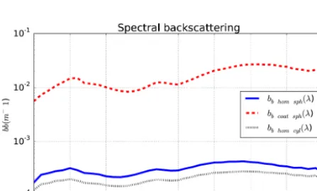
Figure 19.Spectral backscattering for the three test cases: homoge-neous sphere, coated sphere, and homogehomoge-neous cylinder.

firms that the proper selection of particle shapes is an impor-tant requirement in the modeling of optical properties.

This study has pointed at three important lines for future research:

1. All the test cases are synthetic examples that, presum-ably, are simpler than real life. Further work is

communities and the spectral shape of the absorption coefficient.

When dealing with actual phytoplankton, a critical issue is the instrumental accuracy. The attenuation and scat-tering coefficients are key inputs for all retrieval meth-ods, in order to retrieve valid refractive indices. How-ever, as stated by Ramírez-Pérez et al. (2015), the ac-ceptance angle of optical instruments severely affects the amplitude of the measurements. By comparing the extinction coefficient of two instruments with different acceptance angles, disparate magnitude values were ob-tained, with an average ratio of 0.67. Accurate measure-ments are a requirement for obtaining reliable results with the presented methodology.

2. The accuracy of the inversion methods could be im-proved by applying the T-Matrix method to new par-ticle shapes. For instance, coated cylinders could repre-sent algae with cylindrical shape (coated spherical par-ticles generate backscattering functions closer to those produced by actual phytoplankton particles Bernard et al., 2009), or other axially symmetric designs could replicate the actual shape of some phytoplankton par-ticles (as commented before, the T-Matrix approach allows using particle shapes with axial symmetry Sun et al., 2016).

3. Ocean optics goes from research at a microscopic scale (as shown in this paper) to remote sensing, measuring the reflected or backscattered radiation in large areas. The inversion methods based on Lorenz–Mie and T -Matrix approaches could be extended to consider other type of optical measurements, aside from the IOPs, such as the remote-sensing reflectance. As an exam-ple, Fig. 19 shows the spectral backscattering for the three test cases: the homogeneous sphere, the coated sphere, and the homogeneous cylinder. Many opera-tional remote-sensing inversion models for IOPs use im-plicit or exim-plicit assumptions on the refractive index. Hence, their output would likely improve when com-bined with the inversion methods presented here. Re-trieving the index of refraction from space would im-prove the ability to distinguish different oceanic sources of backscattering, but certainly require a much more complex inversion scheme.

To conclude, the results presented in this paper and sum-marized in Table 2, do not determine which is the best method to estimate the phytoplankton optical properties, since none of them are a realistic representation of real algae with cell walls, chloroplasts, vacuoles, nuclei, and other in-ternal organelles, each with its own optical properties. How-ever, the assumed particles serve as a first approximation to actual phytoplankton and are useful to extract some prelimi-nary conclusions and to introduce improvements in order to

obtain approximations closer to reality. Most of the methods shown in this paper are already being used for the retrieval of the refractive indices of isolated particles or bulk oceanic distributions, and their performance can be compared using well-known models. It has been shown that the genetic algo-rithm model is not a fast technique, since it requires several minutes for each estimation (when using spherical shapes, and longer for aspherical particles) as compared to the few seconds generally required by other methods, with the Twar-dowski model being the faster one. However, the genetic al-gorithm is a versatile technique that alone, or combined with other methods, improves the accuracy of the results to a level not achieved by any other method.

6 Conclusions

The accuracy of different inverse methods retrieving refrac-tive indices from the optical properties of small scatterers, and their particle size distribution, has been analyzed. To this end, three different synthetic examples were constructed, each one with a different shape and distribution. The selected shapes were homogeneous spheres, coated spheres, and ho-mogeneous cylinders. The results indicate that the most accu-rate methods are those using a genetic algorithm to optimize the inversion, although they were also the slowest ones. In particular, an excellent agreement was obtained between the estimated and actual refractive indices and volume scattering functions for the homogeneous and coated sphere cases, and a fair agreement for the homogeneous cylinders. The results suggest that even better characterizations could be obtained for the actual phytoplankton optical properties. A next step should be the analysis of the performance of these methods when applied to measurements of isolated cultures of phyto-plankton.

Acknowledgements. This work was supported by the Spanish

National Research Council (CSIC) under the EU Citclops Project (FP7-ENV-308469), the MESTRAL project (CTM2011-30489-C02-01), and the CSIC ADOICCO project (Ref 201530E063). The authors would also like to show their gratitude to Laura Pelegrí, Jimena Uribe, Josep Lluís Pelegrí, and Miquel Ribó for the English revision, as well as to Emmanuel Boss and two anonymous reviewers for their comments and suggestions, which helped to enhance the quality of the manuscript.

Edited by: E. Boss

Reviewed by: two anonymous referees

References

Aas, E.: Refractive index of phytoplankton derived from its metabo-lite composition, J. Plankton Res., 18, 2223–2249, 1996. Aden, A. and Kerker, M.: Scattering of electromagnetic waves from

Bernard, S., Probyn, T., and Barlow, R.: Measured and modelled optical properties of particulate matter in the southern Benguela, South African J. Sci., 97, 410–420, 2001.

Bernard, S., Probyn, T. A., and Quirantes, A.: Simulating the optical properties of phytoplankton cells using a two-layered spherical geometry, Biogeosciences Discuss., 6, 1497–1563, doi:10.5194/bgd-6-1497-2009, 2009.

Bhandarkar, S., Zhang, Y., and Potter, W.: An edge detection technique using genetic algorithm-based optimization, Pattern Recognition, 27, 1159–1180, 1994.

Bohren, C. and Huffman, D. (Eds.): Absorption and scattering of light by small particles, New York: Wiley, Oxford, 1998. Boss, E., Pegau, W., Gardner, W., Zaneveld, J., Barnard, A.,

Twar-dowski, M., Chang, G., and Dickey, T.: Spectral particulate atten-uation and particle size distribution in the bottom boundary layer of a continental shelf, J. Geophys. Res., 106, 9509–9516, 2001a. Boss, E., Twardowski, M., and Herring, S.: Shape of the particulate beam attenuation spectrum and its inversion to obtain the shape of the particulate size distribution, Appl. Opt., 40, 4885–4893, 2001b.

Boss, E., Pegau, W., Lee, M., Twardowski, M., Shybanov, E., Korotaev, G., and Baratange, F.: Particulate backscatter-ing ratio at LEO 15 and its use to study particles com-position and distribution, J. Geophys. Res., 109, C01014, doi:10.1029/2002JC001514, 2004.

Bricaud, A. and Morel, A.: Light attenuation and scattering by phy-toplanktonic cells: a theoretical modeling, Appl. Opt., 25, 571– 580, 1986.

Bricaud, A., Zaneveld, J., and Kitchen, J.: Backscattering efficiency of coccol-25 ithophorids: use of a three-layered sphere model, in: Ocean Optics XI Proc SPIE, 27–33, 1992.

Carder, K., Betzer, P., and Eggimann, D. W. (Eds.): Physical, chem-ical, and optical measures of suspended particle concentrations: Their intercomparison and application to the west African shelf, in: Suspended Solids in Water, Springer US, Oxford, 1974. Choi, W., Fang-Yen, C., Badizadegan, K., Oh, S., Lue, N., Dasari,

R., and Feld, M.: Tomographic phase microscopy, Nature Meth-ods, 4, 717–719, 2007.

Ciotti, A., Lewis, M., and Cullen, J.: Assessment of the relation-ships between dominant cell size in natural phytoplankton com-munities and the spectral shape of the absorption coefficient, Limnol. Oceanogr., 47, 404–417, 2002.

Clavano, W., Boss, E., and Karp-Boss, L.: Inherent optical proper-ties of non-spherical marine-like particles – From theory to ob-servation, Oceanography and Marine Biology: An Annual Re-view, 45, 1–38, 2007.

Dall’Olmo, G., Westberry, T. K., Behrenfeld, M. J., Boss, E., and Slade, W. H.: Significant contribution of large particles to optical backscattering in the open ocean, Biogeosciences, 6, 947–967, doi:10.5194/bg-6-947-2009, 2009.

Fortin, F., Rainville, F. D., Gardner, M., Parizeau, M., and Gagné, C.: DEAP: Evolutionary algorithms made easy, Machine Learn-ing Res., 13, 2171–2175, 2012.

Gordon, H. and Morel, A.: Remote assessment of ocean color for interpretation of satellite visible imagery: A review, Springer Sci-ence and Business Media, 2012.

Greenhalgh, D. and Marshall, S.: Convergence Criteria for Genetic Algorithms, J. Comput., 30, 269–282, 2000.

Hahn, S. L.: Hilbert transforms in signal processing, Artech House on Demand, 1996.

Hale, G. and Querry, M.: Optical constants of water in the 200-nm to 200-µm wavelength region, Appl. Opt., 12, 555–563, 1973. Hold-Geoffroy, Y., Gagnon, O., and Parizeau, M.: Once you

SCOOP, no need to fork, in: Proceedings of the 2014 Annual Conference on Extreme Science and Engineering Discovery En-vironment, 60 pp., ACM, 2014.

Kirk, J. T.: Light and photosynthesis in aquatic ecosystems, Cam-bridge University Press, 1994.

Latimer, P.: Light scattering by a homogeneous sphere with radial projections, Appl. Opt., 23, 442–447, 1984.

Lorenz, L.: Sur la lumière réfléchie et réfractée par une sphère (sur-face) transparente, vol. I of Oeuvres scientifiques de L. Lorenz. Revues et annotées par H. Valentiner, Librairie Lehmann et stage, Copenhagen, 1898.

Mera, N., Elliott, L., and Ingham, D. B.: A multi-population ge-netic algorithm approach for solving ill-posed problems, Com-putational Mechanics, 33, 254–262, 2004.

Meyer, R.: Light-scattering from biological cells – Dependence of backscatter radiation on membrane thickness and refractive in-dex, Appl. Opt., 18, 585–588, 1979.

Mie, G.: Beiträge zur Optik trüber Medien, speziell kolloidaler Met-allösungen, Ann. Phys., 330, 37–445, 1908.

Mischenko, M. and Travis, L.: Capabilities and limitations of a current Fortran implementation of the T-matrix method for ran-domly oriented, rotationally symmetric scatterers, Quant. Spec-trosc. Radiat. Transfer, 60, 309–324, 1998.

Mischenko, M., Travis, L., and Mackowski, D.: T-matrix compu-tations of light scattering by nonspherical particles: a review, Quant. Spectrosc. Radiat. Transfer, 55, 535–575, 1996. Mobley, C., ed.: Light and Water: Radiative Transfer in Natural

Wa-ters, Academic Press, 1994.

Morel, A.: Diffusion de la lumiere par les eaux de mer; resultats experimentaux et approche theorique, Optics of the Sea, AGARD Lecture Ser., 61, 3.1.1.–3.1.76, 1973.

Mugnai, A. and Wiscombe, W.: Scattering from nonspherical Chebyshev particles. I: cross sections, single-scattering albedo, asymmetry factor, and backscattered fraction, Appl. Opt., 25, 1235–1244, 1986.

Nocedal, J. and Wright, S. (eds.): Numerical Optimization, New York : Springer, 1999.

Quirantes, A.: A T-matrix method and computer code for randomly oriented, axially symmetric coated scatterers, Quant. Spectrosc. Radiat. Transfer, 92, 373–381, 2005.

Quirantes, A. and Bernard, S.: Light scattering by marine algae: two-layer spherical and nonspherical models, Quant. Spectrosc. Radiat. Transfer, 89, 311–321, 2004.

Quirantes, A. and Bernard, S.: Light-scattering methods for mod-elling algal particles as a collection of coated and/or nonspherical scatterers, Quant. Spectrosc. Ra., 100, 315–324, 2006.

Ramírez-Pérez, M., Röttgers, R., Torrecilla, E., and Piera, J.: Cost-effective hyperspectral transmissometers for oceanographic ap-plications: performance analysis, Sensors, 15, 20967–20989, 2015.

Signal Processing: Evolution in Remote Sensing (WHISPERS), IEEE, 2014.

Stramski, D., Morel, A., and Bricaud, A.: Modeling the light at-tenuation and scattering by spherical phytoplanktonic cells: a re-trieval of the bulk refractive index, Appl. Opt., 27, 3954–3956, 1988.

Stramski, D., Bricaud, A., and Morel, A.: Modeling the inherent optical properties of the ocean based on the detailed composition of the planktonic community, Appl. Opt., 40, 2929–2945, 2001. Stramski, D., Boss, E., Bogucki, D., and Voss, K.: The role of

seawater constituents in light backscattering in the ocean, Prog. Oceanogr., 61, 27–56, 2004.

Sun, B., Kattawar, G., Yang, P., Twardowskic, M., and Sullivan, J.: Simulation of the scattering properties of a chain-forming tri-angular prism oceanic diatom, Quant Spectrosc Radiat Transfer, available online, 2016.

Twardowski, M., Boss, E., Macdonald, J., Pegau, W., Barnard, A., and Zaneveld, J.: A model for estimating bulk refractive index from the optical backscattering ratio and the implications for un-derstanding particle composition in case I and case II waters, J. Geophys. Res.-Oceans, 106, 14129–14142, 2001.

van de Hulst, H. (Ed.): Ligh scattering by small particles, New York : Wiley, Oxford, 1957.

Volz, F.: Die optik und meteorologie der atmosphärishen trubung, Ber. Dtsch. Wetterdienstes, 13, 1–47, 1954.

Waterman, P.: Matrix formulation of electromagnetic scattering, Proceedings of the IEEE, 53, 805–812, 1965.

Wiscombe, W. and Grams, G.: The backscatered fraction in two-stream approximations, J. Atmos. Sci., 33, 2440–2451, 1976. Zaneveld, J. and Kitchen, J.: The variation in the inherent optical

properties of phytoplankton near an absorption peak as deter-mined by various models of cell structure, Geophys. Res., 100, 13309–13320, 1995.