https://doi.org/10.5194/ars-15-231-2017
© Author(s) 2017. This work is distributed under the Creative Commons Attribution 3.0 License.
Large-baseline InSAR for precise topographic mapping:
a framework for TanDEM-X large-baseline data
Muriel Pinheiro, Andreas Reigber, and Alberto Moreira
German Aerospace Center (DLR), Microwaves and Radar Institute, Oberpfaffenhofen, 82234 Wessling, Germany
Correspondence to:Muriel Pinheiro ([email protected])
Received: 15 December 2016 – Revised: 28 April 2017 – Accepted: 16 May 2017 – Published: 21 September 2017
Abstract.The global Digital Elevation Model (DEM) result-ing from the TanDEM-X mission provides information about the world topography with outstanding precision. In fact, per-formance analysis carried out with the already available data have shown that the global product is well within the require-ments of 10 m absolute vertical accuracy and 2 m relative ver-tical accuracy for flat to moderate terrain. The mission’s sci-ence phase took place from October 2014 to December 2015. During this phase, bistatic acquisitions with across-track sep-aration between the two satellites up to 3.6 km at the equa-tor were commanded. Since the relative vertical accuracy of InSAR derived elevation models is, in principle, inversely proportional to the system baseline, the TanDEM-X science phase opened the doors for the generation of elevation mod-els with improved quality with respect to the standard prod-uct. However, the interferometric processing of the large-baseline data is troublesome due to the increased volume decorrelation and very high frequency of the phase varia-tions. Hence, in order to fully profit from the increased base-line, sophisticated algorithms for the interferometric process-ing, and, in particular, for the phase unwrapping have to be considered. This paper proposes a novel dual-baseline region-growing framework for the phase unwrapping of the large-baseline interferograms. Results from two experiments with data from the TanDEM-X science phase are discussed, corroborating the expected increased level of detail of the large-baseline DEMs.
1 Introduction
Synthetic Aperture Radar Interferometry (InSAR) is a well established remote sensing technique widely employed for the retrieval of topographic information (Bamler and Hartl, 1998; Moreira et al., 2013). Several spaceborne and air-borne SAR systems have been actively acquiring interfero-metric data in the past decades. Among those, the TanDEM-X (TerraSAR-TanDEM-X add-on for Digital Elevation Measurements) stands out as a single-pass bistatic radar mission designed to deliver a highly accurate Digital Elevation Model (DEM) with 90 % point-to-point relative vertical error smaller than 2 m for areas of moderate terrain, and smaller than 4 m for steep areas on a grid of around 12 m by 12 m spacing (Krieger et al., 2007, 2013).
In October 2014, after successfully completing the data acquisition for the construction of the standard global DEM (Zink et al., 2014, 2016), the TanDEM-X mission has en-tered its science phase. During this phase, acquisitions with very large across-track separation between the two satellites have been performed in both pursuit monostatic and bistatic modes (Hajnsek and Busche, 2014; Buckreuss and Zink, 2016). Such configurations enable the generation of local DEMs with higher horizontal and/or vertical accuracies than the standard TanDEM-X products. In fact, with proper com-bination of baselines and tuning of the system parameters, products fulfilling the HRTI-4 standard (i.e., 6 m posting and relative vertical accuracy of less than 0.8 m) can be achieved (Wessel et al., 2016; Pinheiro and Reigber, 2016).
al-z
y 𝐵𝐵1
Master
Slave 1 𝐵𝐵2
Slave 2
𝒌𝒌𝒔𝒔𝟏𝟏
𝒌𝒌𝐦𝐦 𝒌𝒌𝐦𝐦− 𝒌𝒌𝒔𝒔𝟏𝟏 𝒌𝒌𝒔𝒔𝟐𝟐
𝒌𝒌𝐦𝐦
𝒌𝒌𝐦𝐦− 𝒌𝒌𝒔𝒔𝟐𝟐
Master iso-range Multiple scattereres
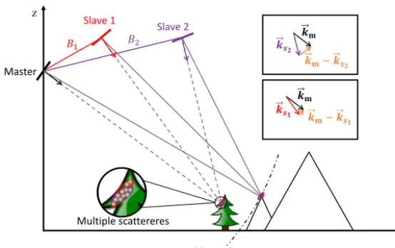
Figure 1.Pictorial representation of an interferometric SAR system composed of one master (in black) and two slaves (in red and purple).
The larger the baseline, the greater the difference between master and slave wavevectors is and, consequently, the higher the sensitivity of
the interferometric phase to increments in thezandydirections. When penetration occurs, e.g., over vegetated areas, multiple scatterers fall
into the same resolution cell decreasing the quality of the interferometric measurements.
ternative for the calibration of orbital errors using the com-plex interferograms is briefly addressed. Finally, the eleva-tion models obtained from two experiments are discussed, each experiment composed of two large-baseline TanDEM-X acquisitions.
2 Large-baseline SAR interferometry: potentials and limitations
Figure 1 shows a pictorial representation of an interferomet-ric SAR system composed of one master (in black) and two slaves (in red and purple). The difference between master and slave viewing geometries due to the spatial baseline al-lows for the separation of scatterers located at the same range distance from one sensor (e.g., along the master iso-range), but having distinct heights above ground. As shown in the picture, the larger the baseline, the greater the difference be-tween master and slave wavevectors (km,ks1 andks2) is and,
consequently, the higher the phase variation induced by in-crements in the z and y directions. Moreover, when pen-etration occurs, e.g., when imaging semitransparent media such as forest or ice, multiple scatterers fall into the same resolution cell. In this case, the interferometric measurement has increased uncertainty, hindering the retrieval of accurate topography, as discussed later in this section. Finally, note that the height information retrieved with SAR interferome-try corresponds to the radar phase center. When employing shorter wavelengths, e.g., Ka-band, the penetration is lim-ited, and the retrieved model is closer to asurface model. On the other hand, when transmitting longer wavelengths, e.g., P-band, the wave penetrates deeper into the medium, and the retrieved model is closer to aterrain model.
The relative height accuracy of elevation models obtained through SAR interferometry is given by
σh= h2π
2π σφ, (1)
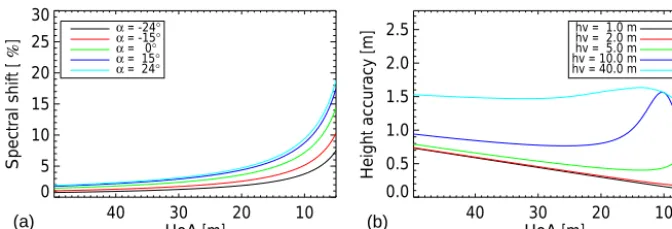
whereh2π is the height of ambiguity (HoA), i.e., the height variation corresponding to a 2π change in the interferomet-ric phase; andσφ is the standard deviation of the phase er-rors (Krieger et al., 2007). Since the height of ambiguity is inversely proportional to the baseline, large baseline acqui-sitions can, in theory, yield DEMs with improved quality. However, the typical increase of the interferometric phase noise in datasets acquired with large baselines limits the effective improvement. The quality deterioration is mainly caused by the increase of baseline and volume decorrelation. Baseline decorrelation occurs due to the spectral mismatch in range caused by the different viewing geometries of master and slave. In principle, it can be avoided by properly filter-ing the range spectrum durfilter-ing the processfilter-ing, at the expense of the range resolution and, consequently, the available num-ber of looks (Reignum-ber, 1999). The plot in the left column of Fig. 2 depicts the percentage of valid bandwidth lost due to the spectral shift, and its variation with the HoA for different local terrain slopes (α). For the simulation, an X-band system with a range bandwidth of 150 MHz is considered (i.e., the value used for the large-baseline TanDEM-X acquisitions), and the off-nadir angle is 44◦. For the simulated parameters, a maximum bandwidth loss and, consequently, reduction of the number of looks of around 20 % can be expected.
40 30 20 10 HoA [m]
0 5 10 15 20 25 30
Spectral shift [
%
] αα = -24 = -15°° α = 0° α = 15° α = 24°
40 30 20 10
HoA [m] 0.0
0.5 1.0 1.5 2.0 2.5
Height accuracy [m]
hv = 1.0 m hv = 2.0 m hv = 5.0 m hv = 10.0 m hv = 40.0 m
(a) (b)
Figure 2.On the left, the percentage of lost bandwidth due to the spectral shift as a function of the height of ambiguity (HoA) is given for
different local terrain slopes (α). On the right, the effect of volume correlation in the relative height accuracy as a function of the HoA is
shown for different volume extents.
avoided (Treuhaft and Siqueira, 2000). The scatterers at dif-ferent heights within the resolution cell have difdif-ferent phase contributions, which are more or less alike according to the system HoA. The volume decorrelation is then given by the integration of all contributions, i.e.,
γvol=
hv
R
0
expjh2π
2πz
f (z)dz
hv
R
0 f (z)dz
=
hv
R
0
expj2λRπ Bsincosθθzf (z)dz
hv
R
0 f (z)dz
, (2)
whereB is the baseline between master and slave acquisi-tions,λis the wavelength,θis the mean incidence angle,Ris the slant range distance,hvis the vertical extent of the
vol-ume andf (z)describes its vertical structure. In the right side of Fig. 2, the effect of volume decorrelation on the relative height accuracy of products generated with SAR interferom-etry is seen. Also for this plot an off-nadir angle of 44◦ is used. Moreover, an exponential model forf (z)with extinc-tion factor of 0.5 dB m−1and underlying SNR decorrelation of 0.95 are considered, values consistent with the TanDEM-X scenario (Kugler et al., 2010; Krieger et al., 2013). The simulation shows that for volume extents of less than 2 m, the relative height accuracy decreases monotonically with the HoA. However, as the volume extent increases, the quality of the height measurement actually degrades with the increase of baseline (or decrease of HoA), i.e., large-baseline short-wavelength interferometers are not able to accurately retrieve the topography over such media. Moreover, as demonstrated in De Zan et al. (2012), Eq. (2) does not fully justify the decorrelation observed over vegetated areas in TanDEM-X products. In fact, the distribution of the scatterers within the resolution cell can further degrade the coherence, deeming large-baseline data over forested areas virtually unusable.
A further challenge for the handling of large-baseline in-terferograms concerns their elevated fringe frequency. The small height of ambiguity causes large phase variations be-tween neighboring pixels, which associated with elevated noise can prevent the retrieval of phase uniqueness. A poorly executed phase unwrapping may introduce large-scale er-rors, hindering the achievable absolute accuracy. Moreover, certain adopted phase unwrapping strategies, e.g., based on maximum-likelihood (ML) estimation, can introduce salt-and-pepper errors due to pixel-wise unwrapping errors, thus compromising the obtained relative vertical accuracy.
The unwrapping of data from the TanDEM-X science phase can profit from the use of the standard TanDEM-X product as a reference height model to flatten the phase. Nev-ertheless, areas of challenging terrain might still be affected by unwrapping errors. For path-following unwrapping algo-rithms, the increased decorrelation over volume scatterers can be particularly problematic, causing the phase unwrap-ping to diverge even when using a priori height informa-tion. Hence, it is interesting to employ unwrapping strate-gies which are able to properly circumvent low-coherence regions. The alternative proposed here is a dual-baseline ex-tension of the region-growing algorithm first presented in Xu and Cumming (1999).
2.1 Dual-baseline region-growing phase unwrapping
Interferometric datasets acquired with different baselines or carriers have different heights of ambiguity. In principle, by properly combining all available interferograms, it is possi-ble to eliminate or reduce the ambiguity of the interferomet-ric phase.
a-posteriori extensions in order to incorporate contextual in-formation. ML approaches are able to provide good height estimates, but their performance can be severely impacted if only a small number of channels is available. The use of con-textual information, e.g., in a maximum a posteriori (MAP) framework, can boost the performance, usually at the ex-penses of computation cost (Ferraiuolo et al., 2009).
For standard TanDEM-X DEM products, an approach to correct unwrapping errors rather than perform a joint phase unwrapping is included in the operational processor (Lachaise et al., 2012; Fritz et al., 2011). Specifically, a dual-baseline configuration is employed using data from the two global coverages, with HoAs of 30 to 35 m and 45 to 50 m, respectively. The approach relies on the easier unwrapping of the differential interferogram, which has a larger HoA of around 100 m. Even if the unwrapped differential phase contains errors, available radargrammetry shifts are accurate enough for their identification and correction. Therefore, an error free reference can be generated and used to correct the data from the individual coverages. The efficiency of the method for the small HoA case considered in this paper is compromised since the differential interferogram has also small HoA and, consequently, cannot always be considered as a reliable reference. Moreover, as discussed before, small HoA data are less coherent, which also impairs the perfor-mance of the operational algorithm.
For the TanDEM-X large-baseline experiment, we pro-pose an adapted dual-baseline region-growing algorithm first developed for airborne repeat-pass InSAR (Pinheiro et al., 2015). The approach intends to obtain unwrapped phases rather than a common height map, and aggregates the dual-baseline redundancy to the spatial growing of unwrapped re-gions (Xu and Cumming, 1999). Moreover, the quality pa-rameters used to choose the unwrapping path are extended to include all available information.
Similarly to the single-baseline region-growing algorithm, the proposed approach is congruent, i.e., only multiples of 2π
are corrected. The ambiguity number of a certain pixel,
namb[p], is calculated based on the phase difference between
the pixel and the already unwrapped neighbors in a prede-fined search window. Here, this search window is extended over a third dimension, i.e., it considers simultaneously the data of the two different baselines. The unwrapped phase values of a certain pixel in both datasets are predicted us-ing three distinct strategies. The first estimation is inherited from the single-baseline region-growing strategy and consid-ers only the local 2-D information, i.e.,
ˆ
ψ{1,2},a[p] =
Pw
kψˆk{1,2}[p] P
wk
, (3)
wherek corresponds to a certain unwrapping direction and
wk accounts for the reliability of its data.ψˆk{1,2}[p]are the unwrapped values estimated from thekth direction, and are
obtained assuming a local linear slope model, i.e.,
ˆ
ψk{1,2}[p] =
ˆ
ψk{1,2}[p−1] +1k{1,2}, (4) where the index [p−1] describes an immediate neighbor, and4k{
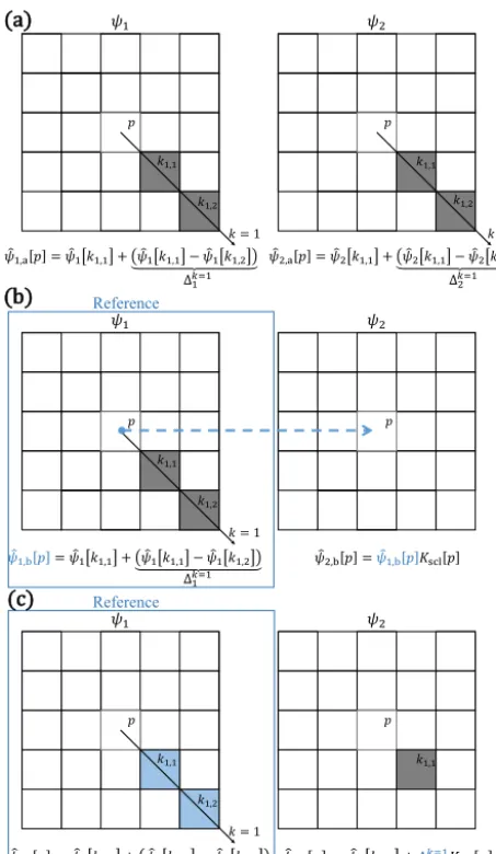
1,2} represents the slope ink calculated considering only the already unwrapped samples. Note that this first esti-mation assumes a certain smoothness of the solution, avoid-ing or mitigatavoid-ing pixel-wise errors. A simple example of the first prediction strategy considering a 5×5 window and a single unwrapping direction is shown in the top row of Fig. 3. In the depiction, the already unwrapped pixels appear in grey. Note that the number and position of available pixels is al-ways the same in both phases since the growing is simul-taneous. On the other hand, the estimations ofψ1,a[p] and ψ2,a[p]are performed independently.
The second prediction considers the data from one of the two acquisitions as the reference, a choice based on the statis-tics of the search window. For this reference, the prediction is calculated using Eqs. (3) and (4). The estimation of the un-wrapped pixel value in the complementary dataset considers a flattening strategy, i.e.,
ˆ
ψ{1,2},b[p] = ˆψ{2,1},a[p]Kscl[p], (5)
whereKscl is a scaling factor accounting for the different
baselines. Note that, if the scaling factorKscl is too large,
e.g., if the interferometric baseline of one dataset is much larger than the one of the other, the noise scaling might be dominant over the slope reduction, discouraging the flat-tening. This is accounted for in the dual-baseline scheme by properly weighting the estimation in Eq. (5) according to expected phase statistics. The plot in the middle row of Fig. 3 illustrates the second prediction strategy considering thatψ1was assigned as reference. The dependence between the two estimates is emphasized by the blue colors. Note that no local information is considered for the computation ofψ2ˆ ,b[p].
Analogously to the previous case, the third prediction strategy also considers the phase with the better local statis-tics as the reference. Once again, the estimation of the un-wrapped value for this dataset is extracted from Eqs. (3) and (4). Additionally, the local slopes of the complementary dataset are evaluated using the reference phase, i.e., for each unwrapping direction
ˆ
ψ{k1,2}[p] =ψˆk{1,2}[p−1] +1k{2,1}Kscl[p]. (6)
The unwrapped pixel value is then extracted from the average of all available directions, as in Eq. (3). If the phase statistics are known and the linear slope model applies, the third guess has an improved slope estimation for the more challenging phase. Moreover, it does not include the assumption of an identical topographic content for both datasets. The plot in the bottom row of Fig. 3 illustrates the third prediction strat-egy. As before, it is considered thatψ1was assigned as
𝑘1,1
𝑘1,2
𝑝 𝜓1
𝑘 = 1 𝑘1,1
𝑘1,2
𝑝
𝜓 2,a𝑝 = 𝜓 2𝑘1,1 + 𝜓 2𝑘1,1 − 𝜓 2𝑘1,2
𝑘 = 1
𝜓 1,a𝑝 = 𝜓 1𝑘1,1 + 𝜓 1𝑘1,1 − 𝜓 1𝑘1,2
𝜓2
Δ1𝑘=1 Δ2𝑘=1
𝑝
𝜓 2,b𝑝 =𝜓 1,b𝑝𝐾scl𝑝
𝜓1 𝜓2
Reference
𝜓 1,b𝑝 = 𝜓 1𝑘1,1 + 𝜓 1𝑘1,1 − 𝜓 1𝑘1,2
𝑘1,1
𝑘1,2
𝑝
𝑘 = 1
Δ1𝑘=1
𝜓 1,c𝑝 = 𝜓 1𝑘1,1 + 𝜓 1𝑘1,1 − 𝜓 1𝑘1,2
𝑝
𝜓 2,c𝑝 = 𝜓 2𝑘1,1 +Δ1𝑘=1𝐾scl𝑝 Reference
𝜓1 𝜓2
𝑘1,1
𝑘1,2
𝑝
𝑘 = 1
𝑘1,1
Δ1𝑘=1 (a)
(b)
(c)
Figure 3. A simple example of phase unwrapping considering a
5×5 window and a single unwrapping direction.(a)depicts the first
prediction strategy, i.e., the estimation is performed independently
on both datasets.(b)illustrates the second prediction strategy, i.e.,
only the reference dataset is locally unwrapped and the
complemen-tary phase is extracted directly from this unwrapped value.(c)
illus-trates the third prediction strategy, i.e., both phases are unwrapped using local information, but the slope estimation is extracted from the reference phase.
phase and re-used for the complementary one, as emphasized by the blue colors.
The use of proper weights is fundamental, and these can be obtained by locally evaluating the interferometric phase statistics. In the following, the computation of weights for the 5×5 search window case represented in Fig. 3 is discussed. For simplicity of notation, it is assumed that the dataset 1 is set as reference in the particular search window, also in accordance to the example presented in Fig. 3.
For the first strategy, the expected variances of the esti-mated unwrapped values are tied to the slope predictions. Considering Eq. (4) and, additionally, assuming the inde-pendence between neighboring samples, 1/w{1,2},ais readily
found as 1/w{1,2},a[p] =
1
K
X
k
2σ{21,2}
qk,1+σ{21,2}
qk,2
, (7)
where K is the number of available unwrapping direc-tions andσ{1,2} are the phase standard deviation values es-timated from the interferometric coherences (Bamler and Hartl, 1998).
For the second prediction strategy, the estimated variances are calculated as
1/w1,b[p] =
1
K
X
k
2σ12
qk,1+σ12
qk,2
, (8)
and
1/w2,b[p] =(Kscl[p]σ1[p])2. (9)
Additionally, the following condition is imposed on Eq. (9),
w2,b[p] =
w2,b[p], if 2σ12 < π
0, if 2σ12=π, (10)
whereσ12is the expected standard deviation of the differen-tial phase given by
σ12=
q
σ22+ Ksclσ12. (11)
Hence, the second prediction is dismissed if the differential noise level is elevated, avoiding noise scaling.
Similarly to Eqs. (7) and (8), the variances corresponding to the third prediction strategy are calculated using the slope statistics, but here considering the reference phase only, i.e., 1/w1,c[p] =
1
K
X
k
2σ12qk,1+σ12
qk,2
, (12)
and
1/w2,c[p] =
1
K
X
k
σ22qk,1+
σ12qk,1+σ12
qk,2
Kscl2 qk,1
. (13)
Using Eqs. (3)–(13), the final prediction of the unwrapped value can be obtained as
ˆ
ψ{1,2}[p] = P
i=a,b,c
ω{1,2},i[p] ˆψ{1,2},i[p]
P
i=a,b,c
ω{1,2},i[p]
, (14)
and the ambiguity number can then be estimated as
ˆ
namb,{1,2}[p] = $ ˆ
ψ{1,2}[p] −φ{1,2}[p] 2π
'
(a)
(b)
(c)
(d)
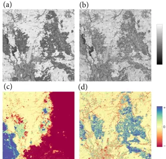
Figure 4.Large-baseline experiment over the region of Kaufbeuren, Germany.(a, b)presents the coherence of the two available datasets,
with heights of ambiguity of approximately 9 and 14 m. (c, d)in the left, the result of the single-baseline Statistical-cost/Network-flow
Algorithm for Phase Unwrapping (SNAPHU). In the right, the result of the dual-baseline region growing algorithm is shown. The large phase errors introduced by the SNAPHU algorithm (red and blue areas) are clearly visible.
whereφ{1,2}[p]are the wrapped phase values.
The single-baseline region growing unwrapping considers the variation of the prediction in different unwrapping di-rections as a reliability measurement for the growing. If the variance is larger than a pre-defined threshold, then the pixel is deemed invalid for the growing iteration, and will be re-evaluated in a later step. For the dual-baseline case, a new reliability metric can be introduced by checking the consis-tence between the three prediction strategies. In this way, a better unwrapping path choice is favored, and, consequently, a more robust unwrapping can be performed. Analytically, the following deviation is computed
εp=max
P
i=a,b,c w1,i[p]
ˆ
ψ1,i[p] − ˆψ1[p]
P
i=a,b,c w1,i[p]
,
P
i=a,b,c w2,i[p]
ˆ
ψ2,i[p] − ˆψ2[p]
P
i=a,b,c w2,i[p]
. (16)
For a reliable unwrapping,εphas to be smaller than a fixed thresholdtεp. Note that if two individual predictions differ
by more thanπ, their associated ambiguity numbers are dis-tinct, i.e., at least one of them would cause an unwrapping error. To promote an easier unwrapping,tεp should not
ex-ceedπ, and should be preferably kept at a fraction of that during the first growing iteration (good results were obtained withεp=π/4). As the growing evolves, more pixels become
available for the prediction, and situations of more challeng-ing unwrappchalleng-ing can be solved. If a pixel fails all the relia-bility tests up to the final growing iteration, it is marked as invalid.
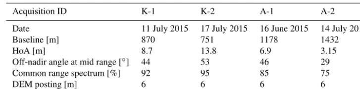
coher-Table 1.Acquisition and processing parameters for Kaufbeuren (K-1 and K-2) and Atacama (A-1 and A-2) experiments.
Acquisition ID K-1 K-2 A-1 A-2
Date 11 July 2015 17 July 2015 16 June 2015 14 July 2015
Baseline[m] 870 751 1178 1432
HoA[m] 8.7 13.8 6.9 3.15
Off-nadir angle at mid range[◦] 44 53 46 29
Common range spectrum[%] 92 95 85 75
DEM posting[m] 6 6 6 6
ence value of around 0.3 and 0.4 in the first and second in-terferograms. The second row of Fig. 4 shows, in the left, the residual unwrapped phase of the first dataset using the Statistical-cost/Network-flow Algorithm for Phase Unwrap-ping (SNAPHU) (Chen and Zebker, 2001). In the right, the dual-baseline region growing result is given. Note that the single-baseline algorithm diverged once it reached the forest, due to the strong decorrelation. Consequently, its result con-tains large unwrapping errors (red and blue regions). On the other hand, the dual-baseline algorithm is able to profit from the weaker decorrelation of the second dataset, providing a better phase unwrapping. Finally, note that even considering the dual-baseline approach, localized residual phase unwrap-ping errors remain, e.g., in the urban areas and should be cor-rected in a posterior step. It is also noteworthy that although the approach is described here considering a dual-baseline scenario, it is also applicable for dual-frequency configura-tions (Pinheiro et al., 2015).
2.2 Interferometric phase calibration
Phase calibration is essential to ensure the absolute accuracy of the height estimates. Moreover, when employing multi-channel approaches, it is crucial that all phases are calibrated in relation to each other or to a common reference. An al-ternative is the use of the global TanDEM-X DEM to create a synthetic phase to be used as reference for the calibration. Assuming that terrain changes are negligible or limited to a small portion of the image, the majority of the interferometric phase content after the removal of the synthetic phase corre-sponds to a global offset or trends due to, e.g., orbital errors (Lachaise and Fritz, 2016). A typical model for the phase er-ror caused by orbital inaccuracies consists of a planar phase ramp, i.e.,
φerr(x, y)=a+bx+cy, (17)
wherex andy represent the range and azimuth coordinates and [a,b,c] are the unknowns to be estimated. Since the pro-cedure has to be carried out prior to the phase unwrapping, the parameters have to be estimated from the complex data. This can be accomplished by exploiting the relationship be-tween range and azimuth local frequencies (fx,fy) and the derivatives of the expected phase error, as discussed in
Pin-heiro et al. (2015) for airborne interferometry. In particular, considering the error model in Eq. (17), (fx,fy) are given by
fx=b/2π, fy=c/2π. (18)
An estimation of the frequencies (fx,fy) can be obtained by locating the maximum of the spectrum of small data blocks. Given the estimated frequencies, the parametersbandcare retrieved by solving Eq. (18) in average. After the removal of the linearly varying components, the estimation of the global offset, e.g., the parameterain Eq. (17), is straightforward.
3 The experiments
As briefly mentioned in Sect. 2.1, the first experiment corre-sponds to data acquired over Kaufbeuren, Germany. The sec-ond experiment correspsec-onds to a mountainous region in the Atacama Plateau, Argentina. Relevant acquisition and pro-cessing parameters are presented in Table 1.
For both experiments, the approach proposed in Sect. 2.1 was employed to jointly unwrap the interferometric phases. However, the DEMs were generated individually for each dataset, i.e., they correspond to a single coverage. On the other hand, the global TanDEM-X DEM is constructed from the average of two or more coverages. In fact, for the test-site over Kaufbeuren, the global TanDEM-X DEM was constructed from 4–5 individual coverages, while for the Atacama case 2–3 coverages were used. Finally, note that each experimental DEM was constructed on a grid of 6 m×6 m posting, i.e., half of the one employed for the global TanDEM-X DEM generation.
Figure 5 shows shaded relief images of a region of inter-est containing agricultural fields and grassland. On the left, the global TanDEM-X DEM is presented. On the right, the large-baseline experimental DEM is shown. The increase in the level of detail is noticeable not only due to improved ver-tical accuracy, but also due to the reduced posting. In the left column of Fig. 6, the histogram of the difference between a reference airborne laser (ALS) terrain model1and the global TanDEM-X DEMs is shown in black. The difference be-tween the DEM corresponding to the largest baseline and the
(a)
(b)
Figure 5.Large-baseline experiment over Kaufbeuren, Germany. The figures show shaded relief images of a region of interest containing
agricultural fields and grassland. (a)The result concerning the global TanDEM-X is presented (posting of 12 m).(b)The result of the
large-baseline experiment is shown (posting of 6 m).
-3 -2 -1 0 1 2 3
[m] 0.0
0.2 0.4 0.6 0.8 1.0
Normalized histogram
TDX expTDX
σTDX=0.32 m
σexpTDX=0.17 m
47.84 47.84 47.85 47.85 47.85 Lat [°]
796 798 800 802 804 806 808
h [m]
TDX expTDX + 2 m ALS + 4 m
47.84 47.85 47.85 47.85 47.85 47.85 Lat [°]
780 790 800 810
h [m]
TDX expTDX + 2 m ALS + 4 m
(a) (b) (c)
Figure 6. (a)The histograms of difference between global DEM and airborne laser (ALS) (black), and DEM constructed from the dataset
acquired with the largest baseline and ALS (red) are presented.(b, c)Profiles of the derived elevation models for different regions of interest
in Kaufbeuren are shown. Offsets of 2 and 4 m were introduced in the experimental TanDEM-X and ALS DEMs to improve the visualization.
ALS model appears in red. For the comparison, an outlier re-moval was carried out to dismiss forest and urban areas, since their information is not contained in the laser terrain model. The corresponding standard deviations are around 32 cm for the global-DEM/ALS difference and of 17 cm for the large-baseline-DEM/ALS, i.e., an improvement is observed even considering the reduced number of looks and coverages. The plots on the middle and right columns of Fig. 6 show two profiles through the DEMs corresponding to grassland and forest, respectively. From the latter, the decrease in vertical accuracy in the large-baseline DEM due to volume decorrela-tion is clear, i.e., the DEM profile in red shows strong height variability caused by the superposition of multiple scatter-ers in the resolution cell. Note that global offsets were in-troduced in the profiles in order to improve the visualization (see legend).
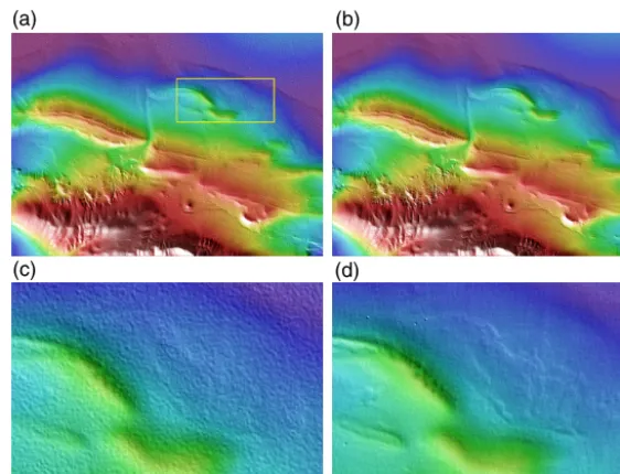
The first row of Fig. 7 shows relief images of a region of interest on the Atacama Plateau containing flat to moder-ate terrain, with total height variation of around 330 m. In the second row, the region within the yellow rectangle is enlarged in order to better visualize the noise reduction. A general improvement of the experimental data in compari-son to the standard one in terms of height noise is notice-able. Again, since the experimental DEM was constructed on a grid with 6 m×6 m sampling, finer details can be re-solved. Finally, note that missing data and unwrapping ar-tifacts due to geometrical effects could not be corrected in
the experimental DEM, since it was constructed using data from a single coverage (and viewing geometry). A few pro-files are shown in Fig. 8, attesting for the good agreement between standard and experimental elevation models, and the improved accuracy of the latter. For this experiment, no ex-ternal reference was available for the quality control and only a relative assessment could be performed. In this case, the large-baseline dataset with lower vertical accuracy (smaller baseline) was chosen as reference (href), and the differences
between the global TanDEM-X (hTDX) and this reference,
and the complementary experimental DEM (hexpTDX) and this reference were evaluated. Assuming that the noise in the elevation models are mutually independent, the standard de-viation of the differences are given by
σTDX2 =σh2
TDX+σ
2
href (19)
and
σexpTDX2 =σh2
expTDX+σ
2
href. (20)
IfσexpTDX< σTDX, it implies that the experimental DEM has
(a) (b)
(c) (d)
Figure 7.Large-baseline experiment over the Atacama Plateau, Argentina. The figures in the first row show relief images of a region of
interest containing flat to moderate terrain (total height variation of around 330 m).(a, c)The result concerning the global TanDEM-X is
presented (posting of 12 m).(b, d)the result of the large-baseline experiment is shown (posting of 6 m). In the second row, the region within
the yellow rectangle is enlarged in order to better visualize the noise reduction.
-3 -2 -1 0 1 2 3
[m] 0.0
0.2 0.4 0.6 0.8 1.0
Normalized histogram
TDX expTDX
σTDX=0.51 m
σexpTDX=0.27 m
-24.79 -24.78 -24.77 -24.76 -24.75 -24.74 -24.73
Lat [°] 3880
3890 3900 3910 3920
h [m]
TDX expTDX + 10 m
-24.69 -24.68 -24.67 -24.66 -24.65 -24.64 -24.63
Lat [°] 3880
3900 3920 3940 3960
h [m]
TDX expTDX + 10 m
(a) (b) (c)
Figure 8. (a)The histograms of difference between global DEM and assigned reference (black), and DEM constructed from the dataset
acquired with the largest baseline and assigned reference (red) are shown.(b, c)Profiles of the derived elevation models for two regions of
interest in the Atacama Plateau are presented. An offset of 10 m was introduced in the experimental DEM to improve the visualization.
shows a standard deviation of around 27 cm, confirming the quality improvement of the experimental data.
4 Conclusions
This paper proposed a new dual-baseline region-growing ap-proach for the phase unwrapping of the data acquired during the TanDEM-X science phase. A detailed analysis of large-baseline DEMs from two experiments has been carried out, attesting the validity of the method. The coherence loss due to volume scattering prevents significant improvement over forested regions, as demonstrated with the Kaufbeuren ex-periment. Nevertheless, for regions covered by low vegeta-tion and bare surfaces, an improvement of the standard de-viation by a factor of two is achieved. Moreover, the large-baseline DEM was constructed on a finer grid, i.e., it contains 4 times more samples than the standard TanDEM-X product.
By means of the proposed approach, a future interferomet-ric SAR mission can be designed with the goal of producing an updated topographic map with an accuracy comparable to that of airborne SAR systems2. Last but not least, existing SAR missions can be enhanced including a constellation of three or more receive-only SAR satellites having small and very large baselines. Such a multistatic SAR concept would allow to generate global high-accurate DEM of the Earth’s surface and to detect topographic changes in the order of decimeters.
2For example, the F-SAR airborne system is able to provide
el-evation models with relative vertical accuracy better than 0.5 m in a
Data availability. The data used in this research was obtained through the TanDEM-X science proposal NTI_INSA6771. In-terested scientists can have access to this data by means of a proposal submission to the TanDEM-X science server https: /tandemx-science.dlr.de.
Competing interests. The authors declare that they have no conflict
of interest.
Acknowledgements. The authors would like to thank the reviewers
for providing valuable comments and suggestions which helped to improve the paper. The TanDEM-X mission is partly funded by the German Federal Ministry for Economic Affairs and Energy (50 EE 1035).
Edited by: Madhu Chandra
Reviewed by: Madhu Chandra and Andreas Danklmayer
References
Bamler, R. and Hartl, P.: Synthetic aperture radar interferometry, Inverse Problems, 14, R1–R54, 1998.
Buckreuss, S. and Zink, M.: TerraSAR-X and TanDEM-X Mission Status, in: Proceedings of EUSAR 2016: 11th European Con-ference on Synthetic Aperture Radar, Hamburg, Germany, 1–6, 6–9 June 2016.
Chen, C. and Zebker, H.: Two-dimensional phase unwrapping with use of statistical models for cost functions in nonlinear optimiza-tion, J. Opt. Soc. Am. A, 18, 338–351, 2001.
De Zan, F., Krieger, G., and Lopez-Dekker, P.: Observations and discussions of TanDEM-X interferogram spectra over rain forest, in: IEEE International Geoscience and Remote Sens-ing Symposium (IGARSS), Munich, Germany, 5554–5557, 22– 27 July 2012.
Ferraioli, G., Shabou, A., Tupin, F., and Pascazio, V.: Multichan-nel Phase Unwrapping With Graph Cuts, IEEE Geosci. Remote Sens. Lett., 6, 562–566, 2009.
Ferraiuolo, G., Meglio, F., Pascazio, V., and Schirinzi, G.: DEM Reconstruction Accuracy in Multichannel SAR Interferometry, IEEE T. Geosci. Remote, 47, 191–201, 2009.
Fornaro, G., Guarnieri, A. M., Pauciullo, A., and De-Zan, F.: Max-imum likelihood multi-baseline SAR interferometry, IEEE Proc. Radar Sonar Navigat., 153, 279–288, 2006.
Fritz, T., Rossi, C., Yague-Martinez, N., Rodriguez-Gonzalez, F., Lachaise, M., and Breit, H.: Interferometric process-ing of TanDEM-X data, in: 2011 IEEE International Geo-science and Remote Sensing Symposium, Vancouver, Canada,
2428–2431, https://doi.org/10.1109/IGARSS.2011.6049701,
24–29 July 2011.
Ghiglia, D. and Wahl, D.: Interferometric synthetic aperture radar terrain elevation mapping from multiple observations, in: Sixth IEEE Digital Signal Processing Workshop, Yosemite National Park, USA, 33–36, 2–5 October 1994.
Hajnsek, I. and Busche, T.: TanDEM-X: Science Activities, in: EU-SAR 2014, Proceedings of 10th European Conference on Syn-thetic Aperture Radar, Berlin, Germany, 1–3, 3–5 June 2014.
Krieger, G., Moreira, A., Fiedler, H., Hajnsek, I., Werner, M., You-nis, M., and Zink, M.: TanDEM-X: A Satellite Formation for High-Resolution SAR Interferometry, IEEE T. Geosci. Remote, 45, 3317–3341, 2007.
Krieger, G., Zink, M., Bachmann, M., Bräutigam, B., Schulze, D., Martone, M., Rizzoli, P., Steinbrecher, U., Anthony, J. W., Zan, F. D., Hajnsek, I., Papathanassiou, K., Kugler, F., Rodriguez-Cassola, M., Younis, M., Baumgartner, S., Lopez-Dekker, P., Prats, P., and Moreira, A.: TanDEM-X: A Radar Interferometer with Two Formation Flying Satellites, Acta Astronaut., 89, 83– 98, 2013.
Kugler, F., Sauer, S., Lee, S. K., Papathanassiou, K., and Hajnsek, I.: Potential of TanDEM-X for forest parameter estimation, in: 8th European Conference on Synthetic Aperture Radar, Aachen, Germany, 1–4, 7–10 June 2010.
Lachaise, M. and Fritz, T.: Update of the Interferometric Processing Algorithms for the Tandem-X High Resolution DEMs, in: EU-SAR 2016, Proceedings of 11th European Conference on Syn-thetic Aperture Radar, Hamburg, Germany, 1–3, 6–9 June 2016. Lachaise, M., Fritz, T., Balss, U., Bamler, R., and Eineder, M.: Phase unwrapping correction with dual-baseline data for the TanDEM-X mission, in: IEEE International Geoscience and Re-mote Sensing Symposium (IGARSS), Munich, Germany, 5566– 5569, 22–27 July 2012.
Moreira, A., Prats-Iraola, P., Younis, M., Krieger, G., Ha-jnsek, I., and Papathanassiou, K.: A tutorial on synthetic aperture radar, IEEE Geosci. Remote Sens. Mag., 1, 6–43, https://doi.org/10.1109/MGRS.2013.2248301, 2013.
Pinheiro, M. and Reigber, A.: Improving TanDEM-X DEMs accu-racy using large-baseline data from the science phase, in: Pro-ceedings of EUSAR 2016, 11th European Conference on Syn-thetic Aperture Radar, Hamburg, Germany, 1–6, 6–9 June 2016. Pinheiro, M., Reigber, A., and Lloredo, J.: Improving satellite de-rived DEMs by using Airborne InSAR data: the TanDEM-X/F-SAR case of study, in: 2015 IEEE International Geoscience and Remote Sensing Symposium, Milan, Italy, 26–31 July 2015. Reigber, A.: Range Dependent Spectral Filtering to Minimize the
Baseline Decorrelation in Airborne SAR Interferometry, in: vol. 3, Proceedings of the IEEE International Geoscience and Remote Sensing Symposium (IGARSS), Hamburg, Germany, 1721–1723, 28 June–2 July 1999.
Reigber, A., Scheiber, R., Jager, M., Prats-Iraola, P., Hajnsek, I., Jagdhuber, T., Papathanassiou, K. P., Nannini, M., Aguilera, E., Baumgartner, S., Horn, R., Nottensteiner, A., and Moreira, A.: Very-High-Resolution Airborne Synthetic Aperture Radar Imag-ing: Signal Processing and Applications, Proc. IEEE, 101, 759– 783, 2013.
Shabou, A., Baselice, F., and Ferraioli, G.: Urban Digital Elevation Model Reconstruction Using Very High Resolution Multichannel InSAR Data, IEEE T. Geosci. Remote, 50, 4748–4758, 2012. Treuhaft, R. N. and Siqueira, P. R.: Vertical structure of vegetated
land surfaces from interferometric and polarimetric radar, Radio Science, 35, 141–177, 2000.
Xu, W. and Cumming, I. G.: A Region-Growing Algorithm for In-SAR Phase Unwrapping, IEEE T. Geosci. Remote, 37, 124–134, 1999.
Zink, M., Bachmann, M., Brautigam, B., Fritz, T., Hajnsek, I., Mor-eira, A., Wessel, B., and Krieger, G.: TanDEM-X: The New Global DEM Takes Shape, IEEE Geosci. Remote Sens. Mag., 2, 8–23, 2014.