An MDCT domain three-point interpolation-based low-complexity frequency estimator

(1)

R E S E A R C H

Open Access

An MDCT domain three-point

interpolation-based low-complexity frequency estimator

Yujie Dun

*

, Guizhong Liu and Xingsong Hou

Abstract

Signal frequency estimation is a problem of significance in many applications including audio signal processing. Compressed domain audio frequency estimators that directly use the modified discrete cosine transform (MDCT) coefficients are suitable for low-complexity audio applications. A new frequency estimation approach, which can obtain the estimated value from a simple combination of three MDCT coefficients, is proposed herein. It exploits the underlying relation among adjacent MDCT values and provides a general form of this type of estimators. The estimator manifests obvious computational advantages over other MDCT domain estimators and is suitable for high signal-to-noise ratio (SNR) conditions.

Keywords:Frequency estimation, MDCT, Audio, Low complexity

1 Introduction

Frequency estimation is a basic problem in signal process-ing research and has been widely used in various applica-tions such as economics, meteorology, astronomy, industry, and consumer electronics [1]. In recent years, low-complexity frequency estimators, which are suitable for low-cost applications, have been proposed in addition to so-called high-resolution (or even super-resolution) fre-quency estimation techniques such as Pisarenko [2], MUSIC [3] and ESPRIT [4]. A typical class of the low-complexity algorithms operates in the frequency domain (via discrete Fourier transform, DFT) and uses several DFT bins to obtain the estimated value [5–8].

For audio signals, frequency estimation plays a crucial role in parametric audio processing, which has been re-ported in various applications such as synthesis [9, 10], recognition [11], enhancement [12], and frame-loss con-cealment [13, 14]. In particular, in audio coding, the fol-lowing two major profiles in MPEG-4 audio coding are based on the sinusoidal analysis of an audio signal: HILN (Harmonic and Individual Lines plus Noise) [15] and SSC (SinuSoidal Coding) [16]. Using the low-complexity fquency estimator can effectively lower the resource re-quirement of the entire processing system, which is significant for massive amount multimedia data processing

and portable ultra-low-power media devices. However, the aforementioned frequency estimation algorithms are not applicable for most low-cost audio applications.

Audio data that are used in most audio applications are stored and transmitted in compressed format, but the compression is not based on DFT. Thus, estimating the parameters of an audio signal, which includes the frequency estimation, is considerably complex. The time-domain signal samples should first be recovered from the compressed data before the estimation, but the recovery generally has a relatively high degree of compu-tational complexity. For high-quality audio compression standards such as MPEG2/4 AAC, Dolby AC-3, WMA, and IETF Opus, the compression is conducted in the modified discrete cosine transform (MDCT) [17] do-main, where an overlap of 50% between successive blocks and time domain alias cancellation (TDAC) are used to mitigate the block effect. To recover one block of the time samples, the inverse MDCT (IMDCT) of three successive blocks is required. Although the fre-quency estimation algorithm is simple, the IMDCT sig-nificantly adds the computational complexity during the recovery of the time domain samples.

To reduce the complexity, several approaches have been proposed. One is to directly calculate the DFT from MDCT with a fast algorithm [18], and the fre-quency estimation is performed with these DFT values. However, computing the DFT of every block requires * Correspondence:[email protected]

School of Electronic and Information Engineering, Xi’an Jiaotong University, Xi’an, Shaanxi 710049, China

(2)

the MDCT values of the corresponding block, previous block, and succeeding block, which causes an inevitable algorithm delay of one block. Another approach is to use the odd-DFT as an intermediate domain between the time domain and the MDCT domain. The frequency is estimated with the odd-DFT coefficients; then, the MDCT is obtained from the odd-DFT by a simple con-version [19–21]. Using the odd-DFT, the system com-plexity of an audio application can effectively be decreased, but this scheme is not fit for the applications that take the compressed audio as their input. Another approach is to directly estimate the frequency with the MDCT coefficients. With the analysis of the MDCT co-efficients of a sinusoid [22], several MDCT domain esti-mators have been proposed in the last decade [23–25], which shows great convenience for the low-complexity implementation of an estimator. All estimators are based on the ratio of two coefficients using the mapping rela-tionship between the frequency value and the coefficient ratio. Effective estimation is restricted in the monotone mapping region. However, in practice, the noise is un-avoidable, which leads the estimation to the non-monotonic region and produces a wrong result.

The major objective of this paper is to propose a three-point interpolation-based estimator, which avoids the effect of non-monotonic mapping and further re-duces the complexity of the MDCT domain frequency estimator to render a simple method for various applica-tions. The contributions are summarized as follows: (i) derive an analytical expression of the MDCT of a single-tone sinusoid based on the sine window’s centered DFT (CDFT); (ii) propose an MDCT domain three-point interpolation-based low-complexity approach for the sig-nal frequency estimation problem. The proposed algo-rithm estimates the frequency from three MDCT bin values with only simple calculations and is significantly less complex than the existing methods. The method is effective for the sine window case and exhibits an esti-mation error lower than 1 Hz when the signal-to-noise ratio (SNR) is above 20 dB.

This paper is organized as follows. In Section 2, we provide the MDCT analysis of a sinusoid, which is the basis of the MDCT domain estimators. The proposed al-gorithm is presented in Section 3. In Section 4, the Monte-Carlo simulation results are shown and the com-plexity is analyzed. The conclusions are summarized in Section 5.

2 MDCT analysis of sinusoids 2.1 Signal model of the estimation

Audio signals are commonly modeled as a combination of several sinusoidal frequency components, which can be expressed as

sað Þ ¼n X m¼0

P−1

smð Þ ¼n X m¼0

P−1

Amsin 2ð πf_mnþϕ_mÞ; ð1Þ

where n is the signal index; P is the number of compo-nents;Am, fm, and∅_mare the amplitude, normalized fre-quency, and phase of each componentsm(n), respectively. The problem of the audio signal parameter estimation is to obtain the values of each parameter set {Am, fm, ϕ_m} form= 0, 1,…,P−1. In general, the frequency estimation is the most important. These frequencies can be estimated together as most time domain methods do or estimated one by one as the frequency domain methods commonly do. When these components are well separated in the frequency scale, the estimation of each component in the frequency domain can be treated as the problem of esti-mating each single frequency component where all other components act as interference noise. Thus, the signal model may be simplified to a single-component model. In this paper, we concentrate on the frequency estimation of a single tone.

Given a discrete sinusoid, the single-tone signal is expressed as

s nð Þ ¼Asin 2ð πf nþϕÞ; ð2Þ whereA,f, and∅are the magnitude, frequency, and ini-tial phase of this sinusoid, respectively. Considering the noisy case, the observed signal is

x nð Þ ¼s nð Þ þw nð Þ ¼Asin 2ð πf nþϕÞ þw nð Þ; ð3Þ where w(n) is generally assumed as the additive white Gaussian noise (AWGN) with zero mean and variance σ2

. The SNR isA/(2σ2).

To estimate the parameters in the MDCT domain, the signal x(n) is framed by weighting a window function h(n) of length 2N, which satisfies the Princen-Bradley perfect reconstruction conditions [17], and converted to itsNpoint MDCT coefficients,

X kð Þ ¼X

n¼0 2N−1

x nð Þh nð Þcos π

N nþ

1 2þ

N

2

kþ1

2

;

ð4Þ where k= 0, 1,…,N−1 is the MDCT bin index. The problem of MDCT domain frequency estimation is to estimate the value offfrom MDCT coefficientsX(k).fis commonly expressed as

f ¼ fs

2Nl¼

fs

2Nðl0þδÞ; ð5Þ

wherefsis the sampling frequency,l0∈Zþ0, andδ∈[0, 1) is the integer and fractional part of the digital frequency

l. Thus, the estimation of l is to obtain the values ofl0

(3)

2.2 Generalized MDCT analysis

The MDCT analysis of a sinusoid is the basis of the fre-quency estimator in the MDCT domain. It exhibits the underlying relationship between the MDCT coefficients and the parameters of the sinusoidal signal. This rela-tionship was first explored by Daudet [22] for the sine window case and generalized by Zhang [25] to other window cases. Here, we briefly describe the generalized MDCT analysis. The analysis is similar to that of [25], but the signal model uses Eq. (3).

Considering the noiseless case, the signal is shown in (2); the general form of the MDCT coefficient X(k) of the signal with windowh(n) is the real part of an expres-sionZ(k) in the form of [25]

Z kð Þ ¼A

ffiffiffiffi

N 2

r

⋅ejφ_⋅ _e−j3π

2ðkþ0:5ÞH k−lð Þ þej32πðkþ0:5ÞHð−k−l−1Þ

h i

;

ð6Þ where

φ¼2N−1

2N πl− π

2þϕ: ð7Þ

H(ξ) is the centered discrete Fourier transform (CDFT) of a window functionh(n),

Hð Þ ¼ξ _N1X

n¼0 2N−1

h nð Þe−j2π

2Nðnþ0:5−NÞðξþ0:5Þ; ð₈Þ

where ξ is not restricted to integer. If h(n) is even-symmetric (a common case in MDCT analysis), the values of its CDFTH(ξ) are real. The MDCT coefficient of the signal in (2) is expressed as

X kð Þ ¼A ffiffiffiffi N 2 r ⋅

cos ϕ0− 3π

2 k

⋅H kð −lÞ þð Þ−1 k

sin ϕ0− 3π

2 k

Hð−k−l−1Þ

;

ð9Þ

whereϕ0is defined as

ϕ0¼φ− 3π

4 ¼

2N−1 2N πl−

5π

4 þϕ: ð10Þ

Equation (9) provides the precise result of the MDCT coefficient for a given sinusoidal signal with an arbitrary symmetric window function case.

To build a simple relation between the sinusoidal fre-quency and the MDCT coefficients, we must simplify (9). Such simplification can be performed based on the features of the window and its CDFTH(ξ). The window function has fast fading sidelobes, which makes the sig-nificant values of its CDFT coefficients appear only at approximately ξ= 0 [25]. For k= 0, 1,…,N−1 and l far from 0 or N−1, only the first term in (9) is significant. Thus, the simplified expression of (9) is

X kð Þ ¼A ffiffiffiffi N

2

r

⋅cos ϕ0− 3π

2 k

⋅H kð −lÞ: ð11Þ

2.3 MDCT analysis for sine window case

The sine window is commonly used in audio signal pro-cessing and coding. The frequency estimator for the sine window case is important for practical applications. The analytical expression of the CDFT coefficientH(ξ) for the sine window can be derived; thus, the analytical expression of the MDCT coefficientX(k) can also be derived. The ex-pression of X(k) is the basis of the proposed three-point interpolation-based low-complexity frequency estimator.

The sine window is defined as

hsinð Þ ¼n sin π

2N nþ 1 2

; ð12Þ

where n= 0, 1,…, 2N−1 has the identical length as the MDCT input data. The sine window is even-symmetric, and its CDFT is real-valued. Substituting (12) into (8) and simplifying, we obtain the following expression of the CDFT

Hð Þ ¼ξ sinð Þπξ 2N ⋅

1

sin π

2Nξ

− 1

sin π

2Nðξþ1Þ

!

: ð13Þ

Forξnear 0, which implies that the bin indexkis near the digital frequencyl, Eq. (13) can be approximated as

Hð Þξ ≈_π1⋅_{ξ ξ}sinð Þ_þπξ

1

ð Þ: ð14Þ

Values at ξ= {0, −1} are obtained using L’Hospital’s rule. This approximation leads to an error less than 1.25 × 10−7. Substituting (14) into (11), a simplified MDCT bin valueX(k) is obtained

X kð Þ ¼A_π

ffiffiffiffi N

2

r

⋅_ð_k₋sin_l_Þ½π_kðk₋−_l_þlÞ

1

ð Þ

ð ⋅cos ϕ0− 3π

2 k

:

ð15Þ

This result is the basis of the proposed frequency estimator.

3 Proposed frequency estimator 3.1 General form

To obtain the estimator, we reform (15) as

X kð Þ ¼A_π

ffiffiffiffi

N 2

r

sinð Þπl⋅_ð_k₋_l_Þ 1_k₋_l_þ 1

ð Þ

ð ⋅ −ð Þ1 ðkþ1Þcos ϕ0−

3π 2 k

:

ð16Þ

In (16), X(k) is composed of three parts: a constant

valued part A_π

ffiffiffi N

2

q

sinð Þ, a variable value partπl 1

k−l

(4)

and a phase modulation factor ð Þ−1 kþ1⋅cos ϕ0−32πk

. The phase modulation factor has a period of 4 and can be listed as

k¼ ₋_cos0;_ϕ 1; 2; 3; 4; ⋯

0; −sinϕ0; cosϕ0; sinϕ0; −cosϕ0; ⋯

Thus, takingM kð Þ ¼_{X k}_{ð Þ}1 , for a givenk0, denotingM−= M(k0−2),M0=M(k0), andM+=M(k0+ 2), we construct a combination of these three values in the form of

λ¼b1M þb2M0þb3Mþ

a1M þa2M0þa3Mþ; ð17Þ

where ai and bi (i= 1, 2, 3) are real-valued coefficients. Then, the constant part and phase modulation factor in (15) are canceled out, and only combinations of (k−l)(k

−l+ 1) remain. Defining δ0=l−k0 and substituting it

into (17), we obtain

λ¼ B2δ20þB1δ0þB0

A2δ20þA1δ0þA0

; ð18Þ

where

A2¼a1−a2þa3

A1¼3a1þa2−5a3

A0¼2a1þ6a3

;and

B2¼b1−b2þb3

B1¼3b1þb2−5b3

B0¼2b1þ6b3

:

8 > > < > > : 8

> > < > > :

ð19Þ

If the coefficientsa_iandbiare properly set, a simple

re-lation betweenλandδ0can be obtained andδ0can be es-timated. For example, if we setA2=A1= 0 andB2=B0= 0 by properly selecting the coefficientsa_iandbi, thenλ=δ0 ⋅B1/A0, B1/A0is a constant determined by ai andbi. An

estimation toδ0isλ/(B1/A0). Thus, the frequency value ^l (we use^to denote an estimated value) can be estimated by^l¼k0þδ^0.

3.2 Proposed estimator

In the proposed estimator, k0is set to the index of the maximum MDCT magnitude |X(k)|. δ0 is estimated using the following formula:

δ0¼

3M−þ2M0−Mþ

2M−þ4M0þ2Mþ: ð20Þ

To simplify the computation, we convert formula (20) to a form that directly uses X(k). Fori=−2, 0, 2, denot-ingX(k0+i) asX−, X0, and X+, respectively, we obtain a new form of (20)

δ0¼

3X0Xþþ2X−Xþ−X−X0

2ðX0Xþþ2X−XþþX−X0Þ: ð 21Þ

The key steps of the proposed estimator are summa-rized as follows:

(1)Find the bin index of the MDCT magnitude peak,

^

k0¼ arg maxk X kðj ð ÞjÞ: ð22Þ

(2)Estimateδ0with the MDCT values ofX−,X0, andX

+according to formula (21).

(3)Finally, obtain the estimated value ofl,

^_l_¼_k^₀_þ^_δ₀_: _ð₂₃_Þ

It is noted that (20) is not the only formula to estimate

δ0; we have derived a set of such formulas; for example,

δ0¼

3M−−14M0−Mþ 3M−þ2M0−Mþ

¼6M−−12M0−2Mþ 5M−þ6M0þMþ

¼ 24M−−8Mþ

17M−þ30M0þ13Mþ¼⋯: ð

24Þ

However, the coefficients in (20) are the most suitable for a simple calculation.

4 Results and discussion 4.1 Comparison benchmarks

Four reported MDCT domain estimators [23–26] and one simplified estimator were used as the performance comparison benchmarks. The four reported estimators are as follows:

Merdjani [23], a method based on the analytical expression of the MDCT coefficient;

Zhu [24], a computationally efficient version of [23]; Zhang [25], an envelope-function-based method

with a look-up table (the single-frame-based envelop method without iteration is used); and

Dun [26], an improved version of the above envelope function method.

We have implemented the estimators of Merdjani and Zhu and obtained Zhang’s from its author. Based on our previous work (Dun), we have noticed that all of these esti-mators involve conditional constructs, i.e., the specific al-gorithm is chosen according to one criterion or several criteria. The decision algorithm verifying the criteria and the conditional branch instructions selecting specific algo-rithm increases the complexity of the program flow espe-cially for pipelined processing. Thus, in our verification tests, one additional benchmark, which is a simplified esti-mator derived from Merdjani [23], is used and labeled as

(5)

has no conditional branch (similar to the proposed estima-tor), and the frequency is estimated by,

f ¼ fs

2Nðk0þδÞ

¼ fs

2N k0þ

3þα−pffiffiffiffiffiffiffiffiffiffiffiffiffiffiffiffiffiffiffiffiffiffiffiffiffiffiα2þ₁₄αþ₁ 2 1ð −αÞ

; ð25Þ wherek0is the frequency bin that locates the maximum

of the so-called pseudo-spectrumS(k),

S kð Þ ¼ ffiffiffiffiffiffiffiffiffiffiffiffiffiffiffiffiffiffiffiffiffiffiffiffiffiffiffiffiffiffiffiffiffiffiffiffiffiffiffiffiffiffiffiffiffiffiffiffiffiffiffiffiffiffiffiffiffiffiX kð Þ2_þ _{X k}₋ 1

ð Þ−X kð þ1Þ

½ 2

q

; ð26Þ

k0¼ arg maxk S kð ð ÞÞ; ð27Þ

andαis the ratio of two MDCT coefficients,

α¼− X kð 0−1Þ

X kð 0þ1Þ: ð

28Þ

4.2 Complexity comparison 4.2.1 General

Complexity refers to the resources that an executable program of the algorithm requires; it includes time com-plexity and space comcom-plexity. Here, the time comcom-plexity is compared by accounting the required operations to estimate the frequency, and the space complexity refers to the storage space size required by the algorithm.

To compare the time complexity, operations such as addition, multiplication, division, square root, compari-son, and bit-shift are accounted for each algorithm. Most

Table 1Comparison of the complexity

Estimators Time complexity _complexitySpace

Addition Multiplication Division Comparison Square-root Bit-shift

Merdjani 6 + 2 N 4 + 2 N 3 4 1 + N – –

Zhu 8 3 5 5 1 – –

Zhang 7 1 3 2 – – 4096

Dun 10 1 5 5 – – 6144

Simplified 5 + 2 N 2 + 2 N 2 – 1 + N 1 –

Proposed 5 3 1 – – 3 –

0 0.2 0.4 0.6 0.8 1

10-15 10-10 10-5 100 105

Digital Frequency ( )

MS

E

Mean Square Error

Proposed Merdjani Zhu

Zhang Dun Simplified

0 0.2 0.4 0.6 0.8 1

10-15 10-10 10-5 100 105

Ma

x

E

rr

o

r

Max Error

0 0.2 0.4 0.6 0.8 1

10-15 10-10 10-5 100 105

MS

E

Mean Square Error

0 0.2 0.4 0.6 0.8 1

10-15 10-10 10-5 100 105

Ma

x

E

rr

o

r

Max Error

a

b

(6)

existing MDCT domain frequency estimation algorithms [23–26] consist of two steps: find the frequency bin k0 that corresponds to the integer partl0and estimate the fractional part δ using a decision method. Note that finding the bin index of the peak location is a common step for all algorithms and the operations are identical, so the operations to find this peak are not included in the comparison.

To compare the space complexity, the required space size to store the look-up table is accounted. The required space to locate the variables and intermediate results is not included in the comparison.

4.2.2 The proposed estimator

According to the proposed frequency estimator in Sec-tion 3.2, with the bin index of the maximum |X(k)|, the operations to obtain the estimated value^lis shown in (21), which includes three MDCT-coefficient-multiplications (X_X0, X0X+, and X_X+), three constant-coefficient-multiplications (with 3 and 2), four additions, and one div-ision. A multiplication with numbers such as 2 and 3 is usually substituted by one bit-shift and addition. Thus, in practice, three multiplications, five additions, one division, and three bit-shifts are used. Neither additional informa-tion nor other operainforma-tion is required.

4.2.3 Other MDCT domain estimators

First, all compared estimators find a peak location. [24–26] use other criteria after locating the initial maximum to ob-tain^l0, whereas Merdjani [23] and the simplified estimator locate the maximum of pseudo-spectrum that is converted from MDCT spectrum. The use of a pseudo-spectrum helps to find the exact^l0, but it also adds a certain amount of operations, which must be accounted in the comparison. Then, always with some decision algorithms (particularly in Zhu [24] and Dun [26]), the value of ^δ is solved from a quadratic equation or computed from a look-up table with polynomial fitting.

We have compared the complexity of these methods as shown in Table 1. The given numbers are the typical values of every algorithm. The size of the look-up table relates to the step. The data in the table present how many values should be stored according to a step of 2−13as reported in [26].

Table 1 shows that the proposed estimator only requires several addition, multiplication, and division operations aside from three bit-shift operations (the simplest oper-ation among the list). Neither comparison nor saving space is required. Obviously, the proposed estimator has the lowest complexity. The simplified algorithm has a similar complexity with the proposed estimator if the cal-culation ofS(k) is not considered.

0 0.2 0.4 0.6 0.8 1

100 105

M

SE

Mean Square Error

0 0.2 0.4 0.6 0.8 1

100 105

Ma

x

E

rr

o

r

Max Error

0 0.2 0.4 0.6 0.8 1

100 105

MS

E

Mean Square Error

0 0.2 0.4 0.6 0.8 1

100 105

M

a

x

E

rro

r

Max Error

a

b

(7)

4.3 Simulation results and discussion

Simulations were conducted to verify the proposed fre-quency estimator and compare with other estimators. Herein, the results for both noiseless and noise-polluted cases are presented.

In all simulations, parameters were set according to the audio applications. The block size and window length were set to 2N= 2048, the sampling frequency was fs=

44.1 kHz, and the magnitude wasA= 1. The initial phase

ϕwas randomly generated in the range of (−π, π), which obeyed the uniform distribution. The estimation error of the frequency value, i.e.,ε¼^f−f in Hertz (Hz), wherefis the sinusoidal frequency and^f is the estimated value, was measured by the maximum valueεmaxand mean square error (MSE). An MSE of 0 dB represents an error of 1 Hz.

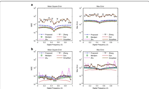
With expression (5), we compared the precision of the estimators whenδvaried from 0 to 1 with a step of 0.05. The signal frequencyl partially decides the model error when simplifies the original form (9) to expression (11); therefore, two values, 46 and 510, were used for its inte-ger part l0in this test. The value of 46 is a bin number that corresponds to approximately 1 kHz according to values off_sandN. The value of 510 is approximately half of the MDCT bin index, which can minimize the inter-ference caused by the negative frequency of a real-valued sinusoidal input. The results of the noise-free condition are shown in Fig. 1.

As expected, both MSE and maximum error are larger for all estimators whenl0= 46. In this frequency domain, the proposed estimator exhibits a slightly larger MSE and maximum error compared to Merdjani, Zhu, and Dun’s methods but significantly less than Zhang’s method and the simplified method. In other words, al-though no conditional construct is used, the proposed estimator exhibits similar precision to the ones that have conditional branches, whereas other existing estimators

significantly lose their accuracy. Whenl0= 510, the max-imum error of the proposed estimator remains similar to other estimators that have conditional branches.

For both cases, the proposed estimator has a slightly lar-ger MSE than the other branched method. The degrad-ation in performance is mainly caused by the third coefficient. In [23, 24, 26], additional decisions are made to select the largest two values. In the proposed estimator, three values are required; neither decision algorithm nor conditional branch instruction is used. Thus, an ultra-low-complexity approach is obtained. Fortunately, the MSE re-mains near or below 10−10for most frequencies.

Then, the corresponding test of the noise-polluted coun-terparts was performed. This test shows the performance of each estimator under the condition of noisy interfer-ence. For the frequency estimation of a real audio signal, the noise originates from other sound sources, environ-mental noise, and other frequency components of the audio signal. For multicomponent signals, the interference

Table 2The description of the 12 MPEG mono sequences

Name Time/s Type

es01 10.73 Suzanne Vega

es02 8.7 Male speech, German

es03 7.6 Female speech, English

sc01 10.97 Haydn trumpet concert

sc02 12.73 Classical orchestral music

sc03 11.55 Contemporary pop music

si01 8 Harpsichord/cembalo

si02 7.73 Castanets

si03 27.89 Pitch pipe

sm01 11.15 Bagpipe

sm02 10.1 Glockenspiel

sm03 13.99 Plucked strings

0 20 40 60 80 100

10-8 10-6 10-4 10-2 100 102

SNR

MS

E

Proposed Merdjani Zhu Zhang Dun Simplified

Fig. 3MSE vs. SNR of different frequency estimators for single-tone sinusoidal input. There were averages of 10,000 runs for each SNR

1.932 1.933 1.934 1.935 1.936 1.937 1.938 1.939 1.94

x 105 -0.25

-0.2 -0.15 -0.1 -0.05 0 0.05 0.1 0.15 0.2 0.25

Sample Index

A

m

p

lit

u

d

e

Original Constructed

(8)

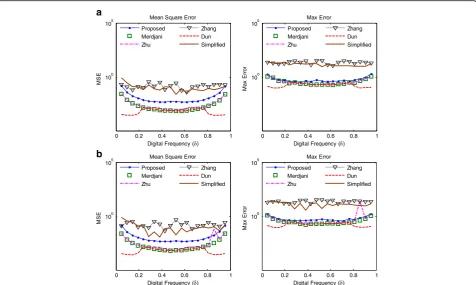
from other frequency components are a major source of noise. The corresponding results with noise of SNR = 40 are shown in Fig. 2. The precision of all estimators signifi-cantly degrades, and MSEs increase from less than 10−10 to greater than 10−3. A level of 10−2is shown for the pro-posed estimator, which corresponds to an error of 0.1 Hz.

A test of MSE vs. SNR was also conducted. In this test, l0 was set to 46, which corresponded to approximately 1 kHz;δwas set to be randomly uniformly distributed in (0, 1). The results are shown in Fig. 3. Basically, for SNR higher than 20 dB, the MSEs of the proposed estimator are less than 1 Hz. The maximum sidelobe level of the sine window is −23 dB; thus, for two frequency compo-nents, a distance greater than one and a half bin guaran-tees that the interference is less than−23 dB. According to the parameter settings, this 1.5 bin distance corre-sponds to 32.3 Hz frequency offset, which is similar to the frequency difference of two music notes: C1 (261.6 Hz) to D1 (293.7 Hz). But in practice, the distance between the notes of a chord is greater than this value. Thus, the proposed estimator is suitable for the low-complexity frequency estimation at such high SNR situation.

4.4 Evaluation with real audio signals

In this part, the proposed algorithm is evaluated with real audio signals. After estimating the major components of

an audio signal with sinusoidal model parameters (fre-quency, amplitude, and phase), the signal is reconstructed by the estimated components. The performances of the various methods are evaluated by comparing the original and the reconstructed signals.

In general, the major components of an audio signal are obtained by the following steps: firstly, finding the largest peak in the spectrum and estimating single-tone parameters from it; secondly, subtracting this estimated tone from the spectrum. These two steps are repeated until all major tones are estimated. This procedure is recommended in multiple component estimation algo-rithms because it enables detection of any tones that are initially masked by leakage from nearby large peaks.

In specific, the frequency of each component is estimated firstly; then, the amplitude and phase are estimated with the method given in Merdjani [23]. The proposed algorithm and the five benchmarks are used to get the estimated frequencies. To make comparison in a uniform framework, the components of an audio signal are esti-mated in the same order by all of the algorithms.

The test has been conducted with audio set that is used in the verification test of MPEG audio, which con-tains 12 mono audio files as listed in Table 2. With a sampling frequency of 48 kHz and frame length of 1024, each frame lasts about 21.3 ms. Maximum component number of 30 and minimum residual energy of 10−4are

Fig. 5Audio quality comparison by MSE. Using the original audio signals as references, MSE of each reconstructed audio is calculated

(9)

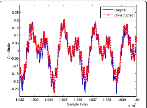
used as criteria to stop component extraction of a frame. An overlap of 50% is used between subsequent frames both in MDCT analysis and in waveform reconstruction. Figure 4 presents a detailed part of the reconstructed signal of“es01”when the proposed frequency estimation algorithm is used, and compares it with the original sig-nal. It can be observed that the reconstructed waveform is almost the same with the original audio.

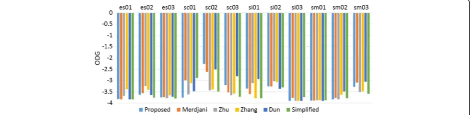
To evaluate the performance of the proposed algo-rithm, not only the errors between the original and the reconstructed signals are compared but also the audio qualities of the reconstructed signals are measured. The errors are compared by using MSE between the original and the reconstructed audio signals, and the result is plotted in Fig. 5. The audio quality is evaluated by using formal objective test with PQevalAudio software, which is used for perceptual evaluation of audio quality (PEAQ) specified in ITU BS.1387-1. The Objective Dif-ference Grade (ODG), which has a range from 0 to −4, is used to indicate the audio quality. A score of 0 means no perceptible difference compared with a reference audio, and a score of−4 means that apparent perform-ance degradation can be perceived. The test results are shown in Fig. 6.

The results of Figs. 5 and 6 show that the performance of the reconstructed audio signal remains similar to other estimators except the two most complexed ones although the proposed algorithm reduces the complexity greatly. The proposed algorithm avoids the spectrum conversion (from MDCT to pseudo-spectrum) used in Merdjani [23] and the simplified algorithm so that the algorithm complexity is irrelevant to the frame lengthN (as shown in Table 1, typical frame length of audio signal is 1024, 512, or so). At the same time, the proposed al-gorithm avoids the conditional constructs, which is beneficial to the speed of a frequency estimator in pipe-lined processor.

5 Conclusions

A low-complexity frequency estimator that operates with three MDCT coefficients and only several simple calcula-tions is proposed in this paper. The analytical expression of the MDCT coefficients, which is the basis of the proposed estimator, is also presented. The proposed estimator shows a great reduction in complexity compared to other MDCT domain estimators and provides a good complexity/per-formance tradeoff. Without using conditional branch in-structions, this estimator is especially fit for pipelined operators.

Funding

This research was supported in part by the National Natural Science Foundation of China under Grants NSFC61173110, NSFC61373113, NSFC61372091, NSFC61671365 and NSFC U1531141.

Authors’contributions

YD was responsible for proposing the algorithm and drafting the manuscript. GL and XH provided the comments on the verification tests and the drafts. All authors have read and approved the final manuscript.

Competing interests

The authors declare that they have no competing interests.

6 Publisher’s Note

Springer Nature remains neutral with regard to jurisdictional claims in published maps and institutional affiliations.

Received: 8 September 2016 Accepted: 29 March 2017

References

1. P Stoica, RL Moses,Spectral analysis of signals(Pearson/Prentice Hall, Upper Saddle River, 2005)

2. VF Pisarenko, The retrieval of harmonics from a covariance function. Geophys. J. Int.33(3), 347–366 (1973)

3. RO Schmidt, Multiple emitter location and signal parameter estimation. Antennas and Propagation IEEE Transactions on34(3), 276–280 (1986) 4. R Roy, T Kailath, ESPRIT-estimation of signal parameters via rotational

invariance techniques. Acoustics, Speech and Signal Processing IEEE Transactions on37(7), 984_–995 (1989)

5. BG Quinn, Estimating frequency by interpolation using Fourier coefficients. Signal Processing, IEEE Transactions on42(5), 1264–1268 (1994) 6. MD Macleod, Fast nearly ML estimation of the parameters of real or

complex single tones or resolved multiple tones. Signal Processing, IEEE Transactions on46(1), 141–148 (1998)

7. E Jacobsen, P Kootsookos, Fast, accurate frequency estimators [DSP Tips & Tricks]. Signal Processing Magazine, IEEE24(3), 123–125 (2007)

8. C Candan, Analysis and further improvement of fine resolution frequency estimation method from three DFT samples. Signal Processing Letters, IEEE

20(9), 913–916 (2013)

9. H Kawahara, I Masuda-Katsuse, A De Cheveigne, Restructuring speech representations using a pitch-adaptive time-frequency smoothing and an instantaneous-frequency-based F0 extraction: possible role of a repetitive structure in sounds. Speech Comm.27(3), 187–207 (1999)

10. EB George, MJ Smith, Speech analysis/synthesis and modification using an analysis-by-synthesis/overlap-add sinusoidal model. Speech and Audio Processing, IEEE Transactions on5(5), 389–406 (1997)

11. A. Eronen, and A. Klapuri, Musical instrument recognition using cepstral coefficients and temporal features. (Acoustics, Speech, and Signal Processing, ICASSP_’00. 2000 IEEE International Conference on, Istanbul, 2000), pp. II753-II756 vol. 2

12. DPN Rodríguez, JA Apolinário, LWP Biscainho, Audio authenticity: detecting ENF discontinuity with high precision phase analysis. Information Forensics and Security, IEEE Transactions on5(3), 534_–543 (2010)

13. S.-U. Ryu, and K. Rose, An mdct domain frame-loss concealment technique for mpeg advanced audio coding. (Acoustics, Speech and Signal Processing, 2007. ICASSP 2007. IEEE International Conference on, Honolulu, 2007), pp. I-273-I-276

14. M.-Y. Zhu, N. Chen, X.-Q. Yu, and W.-G. Wan, Packet Loss Concealment for compressed audio stream using sinusoidal frequency estimation. (Multimedia and Expo (ICME), 2010 IEEE International Conference on, Suntec City, 2010), pp. 316_–321

15. H. Purnhagen, and N. Meine, HILN—the MPEG-4 parametric audio coding tools. (Circuits and Systems, The 2000 IEEE International Symposium on, Geneva, 2000), pp. 201–204

16. A. C. Den Brinker, J. Breebaart, P. Ekstrand, J. Engdegård, F. Henn, K. Kjörling, W. Oomen, and H. Purnhagen, An overview of the coding standard MPEG-4 audio amendments 1 and 2: HE-AAC, SSC, and HE-AAC v2, EURASIP Journal on Audio, Speech, and Music Processing. 2009(3(2009)

17. JP Princen, AB Bradley, Analysis/synthesis filter bank design based on time domain aliasing cancellation. Acoustics, Speech and Signal Processing, IEEE Transactions on34(5), 1153–1161 (1986)

(10)

19. AJS Ferreira,Accurate estimation in the ODFT domain of the frequency, phase and magnitude of stationary sinusoids(Applications of Signal Processing to Audio and Acoustics, 2001 IEEE Workshop, New Platz, 2001), pp. 47–50 20. A. J. Ferreira, and D. Sinha, Accurate and robust frequency estimation in the

ODFT domain. (Applications of Signal Processing to Audio and Acoustics, 2005 IEEE Workshop on New Paltz, NY, 2005), pp. 16_–19

21. Y Dun, G Liu, A fine-resolution frequency estimator in the odd-DFT domain. IEEE Signal Processing Letters22(12), 2489–2493 (2015)

22. L Daudet, M Sandler, MDCT analysis of sinusoids: exact results and applications to coding artifacts reduction. Speech and Audio Processing, IEEE Transactions on12(3), 302–312 (2004)

23. S Merdjani, L Daudet,Direct estimation of frequency from MDCT-encoded files

(Proceedings of the 6th International Conference on Digital Audio Effects, London, 2003), pp. 8_–11

24. M-Y Zhu, W Zheng, D-X Li, M Zhang, An accurate low complexity algorithm for frequency estimation in MDCT domain. IEEE Trans. Consum. Electron.

54(3), 1022–1028 (2008)

25. S Zhang, W Dou, H Yang, MDCT sinusoidal analysis for audio signals analysis and processing. Audio, Speech, and Language Processing, IEEE Transactions on21(7), 1403–1414 (2013)

26. Y Dun, G Liu,An improved MDCT domain frequency estimation method

((Signal and Information Processing (ChinaSIP), 2014 IEEE China Summit & International Conference, Xi’an, 2014), pp. 120–123

Submit your manuscript to a

journal and beneﬁ t from:

7Convenient online submission 7Rigorous peer review

7Immediate publication on acceptance 7Open access: articles freely available online 7High visibility within the ﬁ eld

7Retaining the copyright to your article