© European Geosciences Union 2008
Geophysicae
GALS – Gradient Analysis by Least Squares
M. Hamrin1, K. R¨onnmark1, N. B¨orlin2, J. Vedin1, and A. Vaivads3
1Department of Physics, Ume˚a University, Ume˚a, Sweden
2Department of Computing Science, Ume˚a University, Ume˚a, Sweden 3Swedish Institute of Space Physics, Uppsala, Sweden
Received: 20 May 2008 – Revised: 8 October 2008 – Accepted: 15 October 2008 – Published: 10 November 2008
Abstract. We present a method, GALS (Gradient Analysis
by Least Squares) for estimating the gradient of a physical field from multi-spacecraft observations. To obtain the best possible spatial resolution, the gradient is estimated in the frame of reference where structures in the field are essentially locally stationary. The estimates are refined iteratively by a least squares method.
We show that GALS is not very sensitive to the space-craft configuration and resolves structures much smaller than the characteristic size of the spacecraft distribution. Further-more, GALS requires little user input.
GALS has been tested on synthetic magnetic field data and data from the Cluster FGM instrument. GALS will also be useful for other types of data. The results indicate that GALS is robust and superior to the curlometer method for estimat-ing the current from magnetic field measurements.
Keywords. Space plasma physics (Experimental and
math-ematical techniques; Instruments and techniques) – General or miscellaneous (Techniques applicable in three or more fields)
1 Introduction
The fundamental equations of space physics, such as the MHD equations, Maxwell’s equations, and the Vlasov equa-tion, are all first order differential equations relating the tem-poral evolution to spatial gradients of physical fields. To compare in situ observations with theory we must hence be able to calculate gradients from measurements. In space physics the calculation of space and time gradients from satellite measurements is not a trivial problem. Using a sin-gle spacecraft we can determine how a measured field varies Correspondence to: M. Hamrin
along the satellite orbit, but without complementary infor-mation we cannot tell whether these variations are spatial or temporal. Furthermore, we have no information about gradi-ents in directions perpendicular to the spacecraft orbit. The unique capability of resolving three-dimensional spatial vari-ations was an important motivation for the Cluster mission, comprising four identical spacecraft launched in 2000. De-scriptions of methods for analyzing multi-spacecraft data, for example the curlometer method, the wave telescope technique, and the discontinuity analyzer, are collected in Paschmann and Daly (1998). In this study we will compare GALS to the curlometer and to a single spacecraft method (L¨uhr et al., 1996).
From four simultaneous measurements in space we can obtain reasonable estimates of the spatial derivatives. For example, the curlometer method (Robert et al., 1998) esti-mates the rotation of the magnetic field,∇×B, and
(neglect-ing the displacement current) the correspond(neglect-ing current den-sity j, can be calculated. However, the curlometer cannot estimate spatial variations on length scales smaller than the spacecraft configuration. De Keyser et al. (2007) recently described a method based on least squares fitting for calcu-lating gradients from multi-point observations. This method is demonstrated to be very robust, and it can provide reliable error estimates.
Gradients with scalelengths significantly shorter than the distance between spacecraft can be resolved by combining a discontinuity analysis (Dunlop and Woodward, 1998) to determine the orientation and velocity of the boundary with single spacecraft techniques (L¨uhr et al., 1996) to compute gradients. The spatial resolution of these methods is deter-mined by the data sampling frequency and the velocity of the spacecraft relative to the discontinuity. These methods can produce very good results under favorable conditions, but their application requires significant effort and skill.
3492 M. Hamrin et al.: Gradient analysis
s2 s3 s4
s1
s2
s4
s3
Λ ∆tu
space time
(a)
~L= charac. size of spacecraft config.
space time
(b)
s1
∆t
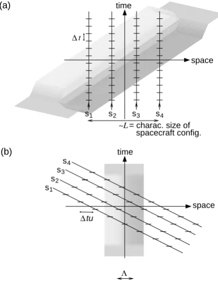
Fig. 1. (a) A current sheet passing four satellites,s1–s4, in the frame
of reference moving with the satellites. (b) The current sheet and the spacecraft in the reference frame moving with the sheet.
J z
x
y
=−15km/s W=20km
Vcs
=5km/s
sat
V
L=200km
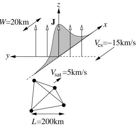
Fig. 2. Setup for a test run on synthetic magnetic field data.
Rela-tive to a fixed reference system, the spacecraft and the structure are moving with+5km/s and−15km/s, respectively.
True GALS Curl SC1 SC2 SC3 SC4
−20 0 20
−1 0 1
0 1
−20 0
24−Dec−2006
15:01:00 15:01:10 15:01:20 15:01:30 15:01:40 1
5 10 50 By [nT
]
jx
[
µ
A
/
m
2]
jz
[
µ
A
/
m
2]
u
(
By
)
[
km
/
s
]
Λ
(
By
)
[
km
]
(a)
(b)
(c)
(d)
(e)
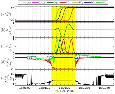
Fig. 3. (a) Magnetic fieldycomponent for the narrow current sheet in Figure 2 as observed by the four satellites. The reconstructed field from GALS (magenta) and the true field (black, dotted) are also shown. (b)–(c) Current densityJxandJz from GALS (magenta), the curlometer (dark green), and the single-spacecraft method (red, yellow, blue, and green). The true current is shown with the black dotted line. (d) GALS estimated structure velocityux,uyanduz (red, green and blue) for theBzcomponent. (e) Resolution parame-terΛ(By)obtained by GALS in the reconstruction ofBy. The high-lighted time window indicates the used coherence timeTc= 12s.
Fig. 1. (a) A current sheet passing four satellites, s1–s4, in the frame
of reference moving with the satellites. (b) The current sheet and the spacecraft in the reference frame moving with the sheet.
estimate spatial gradients on length scales shorter than the characteristic size of the spacecraft configuration. Since GALS is based on weighted least squares similar to those used by De Keyser et al. (2007), it is possible to produce er-ror estimates of comparable quality. However, in this first study we will not discuss error estimates. Instead, we will focus on describing how GALS combines the best features of the curlometer and the De Keyser et al. (2007) methods with the high resolution of the discontinuity analysis/single spacecraft techniques.
The gradients of scalar physical fields are invariant under Galilei transformations. A simple consequence of Galilei in-variance is that there almost always exist a frame of reference where the local time derivative is zero. The only exception is the case when the spatial gradient vanishes. In that particular case the time derivative cannot be transformed away.
The quality of the gradient estimates that can be obtained from spacecraft observations of the field depends crucially on the choice of frame of reference. The best possible esti-mate is obtained in the frame of reference where the field lo-cally appears stationary. Notice that “stationary” here means that the partial time derivative of the physical field is zero at the point in space-time where the gradient is computed. In
this reference frame, time variations at nearby points are also minimized, although they cannot be completely eliminated. As will be explained below, the usually rather high time res-olution obtained from in situ satellite measurements may in this optimal frame of reference be converted into a spatial sampling along the gradient at distances much shorter than the satellite separation.
2 Method
Let the position of satellitesat timet be given by rs=Rs(t ).
In the following, the satellite subscriptswill be omitted un-less it is needed for clarity. Assuming a cluster ofSsatellites, we will estimate the space and time gradients of a physi-cal fieldF along the trajectory Rcm(t )=1SPSs=1Rs(t )of the
center of mass of the satellites. At the reconstruction timetp
the gradients are determined at the point rp=Rcm(tp).
Trans-forming to a frame of reference moving with the velocity
Prp=dtRcm(tp)of the center of mass, we introduce the new
coordinates
τ =t−tp, (1)
x0(τ )=r−rp−τPrp. (2)
Here, τ is the time relative to the reconstruction time and
x0(τ ) is the corresponding spatial coordinates relative to the reconstruction point rp moving with velocity Prp.
Us-ing these substitutions, the function F (r, t )describing the field in the original coordinate system is in the new system replaced byF0(x0, τ )=F (x0(τ )+rp+τPrp, tp+τ )=F (r, t ).
The first derivatives of F0 form a linear approximant FL0(x0, τ )=Fp+x0·∂x00Fp0+τ ∂τFp0to the exactF0, valid for
small x0 and τ. Considering a reference frame moving with velocity u relative to the satellites and introducing the new coordinates xu=x0−uτ, we find that the approximant is transformed into
FLu(xu, τ )=Fpu+xu·∂xuFpu+τ ∂τFpu (3) whereFpu=Fp0=Fp and∂xuFpu=∂x0Fp0=∂xFp are
indepen-dent of the reference frame, but the time derivatives are re-lated by∂τFpu=∂τFp0+u·∂x0Fp0. From this we see that by
choosing a velocity
u= −∂τF 0 p∂xFp
k∂xFpk2
(4) we can always find a reference frame where∂τFpu=0.
As illustrated in Fig. 1, we can convert the temporal res-olution of the observations into a spatial resres-olution by trans-forming to a reference frame where ∂τFpu=0. Figure 1a
shows the situation in the center of mass frame of reference. The satellites sample the field at the discrete timesτn=n1t,
n=0,±1, . . . ,±N. At the timeτnsatellitesis at x0sn=x0s(τn)
and observes the fieldFsn=F0(x0sn, τn). The spatial
coordi-nates x0sn of the satellites are essentially independent ofτn,
[image:2.595.53.278.64.363.2]and take on only four distinct values. While the satellites are at rest, a point of constantFL0moves to the right with velocity
u, that is,FL0(τu, τ )≈Fp.
Figure 1b illustrates the same scene in the reference frame moving with velocity u. At xu=0 the value ofFLuis now time independent andFLu(0, τ )≈Fp to first order inτ. Since the
field is as stationary as possible, the distortion caused by time averaging is minimized in this reference frame. The satellites moving through the structure now provide measurements at the coordinates xusn=x0sn−uτn, with a spatial separationu1t
along the gradient direction. In many cases, this will allow us to resolve the gradient with higher resolution and better statistics than using only four points with separations deter-mined by the satellite configuration.
The field and its derivatives at the reconstruction point are estimated by minimizing the weighted least squares problem
X
s,n h
Fpu+xusn·∂xuFpu+τn∂τFpu−Fsn i2
Wu(xusn, τn), (5)
In this first study, this problem is solved by a simple itera-tive method, described in the Appendix. The Maxwell equa-tion ∇·B=0 is used as constraint in our least squares rou-tines. The weight functionW is initially an isotropic Gaus-sian whose width is determined by the characteristic space-craft separationL, but its width along the gradient will be adjusted in the algorithm to a value3<Lwhenever possi-ble.
The GALS method is designed to optimize the resolution in the direction of the gradient by transforming to a reference frame where∂τFpu=0 and reducing3. The resolution in the
plane perpendicular to the gradient is still determined by the satellite separation, but since this is a plane of minimal field variations the resolution is not critical.
Structures in the observed field will in practice have a finite lifetime. By specifying a parameter, which we call the coher-ence timeTc, the user can to some extent tune GALS to the
problem and the data at hand. In the algorithm, a time win-dow is created by restricting theτ-values toτn≤Tc/2. The
optimal choice will depend on the data at hand, but also on the physical phenomenon of interest. IfTc is chosen longer
that the actual coherence time of relevant structures in the field, it may be impossible to find a meaningful velocity. On the other hand, ifTcis chosen too short, the GALS algorithm
may not be able to interpret data from separate spacecraft as a single, coherent, structure. For a particular feature in the data, it is often possible to estimate a suitableTcby
inspect-ing when and how well this feature is reproduced in the data from the other spacecraft. In practice, it often makes sense to use the rule of thumb thatTcis chosen to match the
“clus-ter transition time”, i.e., the approximate time from when the first spacecraft enters the structure until the last spacecraft leaves it.
3 Results
In this section we present the capacity of GALS as an esti-mator for the current density. The performance of GALS is investigated by using both synthetic and real magnetic field data, and the GALS results are compared with what can be obtained with two other tools for estimating the current: the curlometer(Robert et al., 1998; Dunlop et al., 2002) and the single-spacecraft technique (L¨uhr et al., 1996).
The curlometer uses multi-spacecraft, e.g. Cluster, mag-netic field data to calculate the current density from∇×B
(assuming that the displacement current is negligible in Am-pere’s law). The current is estimated from four simultane-ous measurements of the magnetic field, and the curlome-ter therefore captures the instantaneous current density as a snapshot in time. Since the curlometer technique is based on the assumption that the current is constant over the tetrahe-dral volume defined by the four spacecraft, the spatial reso-lution of the curlometer current density depends directly on the satellite configuration.
The single spacecraft technique can very efficiently re-solve, e.g., thin current sheets when it is combined with a method such as the discontinuity analyzer for obtaining the velocity of the spacecraft relative to the sheet. Consider-ing the sheet to be stationary, the observed total derivative is interpreted as a spatial gradient and the resolution is deter-mined by the data sampling rate rather than by the size of the satellite tetrahedron. The quality of the velocity estimate is of crucial importance when determining the full current density vector with the single-spacecraft technique. When analyzing a convecting, planar, current sheet passing all four spacecraft this is generally not a problem, but investigations of more general current density structures with the single-spacecraft technique are limited by the lack of good velocity estimates. The least squares method for gradient calculation devel-oped by De Keyser et al. (2007) is more robust than the cur-lometer, but they did not explicitly exploit the advantages of a moving reference system. In the absence of signifi-cant correlations between the spacecraft, GALS will calcu-late gradients by a method very similar to that of De Keyser et al. (2007). However, whenever a coherent structure can be found, GALS will automatically attempt to determine its ve-locity and and estimate the gradients by a method related to the single spacecraft technique. We will show that GALS combines the robustness of the least squares method with the high spatial resolution of the single spacecraft technique. We will also show that it is possible to tune the behaviour of GALS to the problem at hand by changing the coherence time,Tc.
3494 M. Hamrin et al.: Gradient analysis
s
2
s
3
s
4
s
1
s
2
s
4
s
3
Λ
∆
tu
space
time
a)
~L
= charac. size of
spacecraft config.
space
time
b)
s
1
∆
t
Fig. 1. (a) A current sheet passing four satellites,
s
1
–
s
4
, in the frame
of reference moving with the satellites. (b) The current sheet and the
spacecraft in the reference frame moving with the sheet.
J
z
x
y
=−15km/s
W=20km
V
cs=5km/s
sat
V
[image:4.595.52.285.61.274.2]L=200km
Fig. 2. Setup for a test run on synthetic magnetic field data.
Rela-tive to a fixed reference system, the spacecraft and the structure are
moving with
+5
km/s and
−
15
km/s, respectively.
True GALS Curl SC1 SC2 SC3 SC4
−20
0
20
−1
0
1
0
1
−20
0
24−Dec−2006
15:01:00
15:01:10
15:01:20
15:01:30
15:01:40
1
5
10
50
B
y [nT]
j
x[
µ
A
/
m
2]
j
z[
µ
A
/
m
2]
u
(
B
y)
[
km
/
s
]
Λ
(
B
y)
[
km
]
(a)
(b)
(c)
(d)
(e)
Fig. 3. (a) Magnetic field
y
component for the narrow current sheet
in Figure 2 as observed by the four satellites. The reconstructed field
from GALS (magenta) and the true field (black, dotted) are also
shown. (b)–(c) Current density
J
x
and
J
z
from GALS (magenta),
the curlometer (dark green), and the single-spacecraft method (red,
yellow, blue, and green). The true current is shown with the black
dotted line. (d) GALS estimated structure velocity
u
x
,
u
y
and
u
z
(red, green and blue) for the
B
z
component. (e) Resolution
parame-ter
Λ(
B
y
)
obtained by GALS in the reconstruction of
B
y
. The
high-lighted time window indicates the used coherence time
T
c
= 12
s.
Fig. 2. Setup for a test run on synthetic magnetic field data.
Rela-tive to a fixed reference system, the spacecraft and the structure are moving with+5 km/s and−15 km/s, respectively.
small compared to the characteristic size of the satellite tetra-hedron,L=200 km. The tetrahedron has elongation and pla-narityE=P=0.75 (Paschmann and Daly, 1998).
Panel (a) of Fig. 3 shows theBy component of the
mag-netic field sampled by the four spacecraft. The other field components are identically zero,Bx≡Bz≡0. The solid
ma-genta line and the dotted black line show the field recon-structed by GALS and the true magnetic field at the center of mass of the satellites. It is evident that GALS reconstructs By correctly although the current sheet is narrow and could
be difficult to resolve. The coherence timeTc is chosen as
12 s, as indicated by the width of the highlighted yellow re-gion.
Panels (b) and (c) show the two non-zero components of the current density estimates, Jx and Jz, obtained from
GALS, the curlometer and the single-spacecraft method, re-spectively. As indicated in Fig. 2, the true current is along the z-direction. However, the curlometer (dark green line) produces an artificialJx, which is bi-polar and comparable
to the true current in magnitude. The correspondingJxfrom
GALS (magenta) is three orders of magnitude smaller and not visible in Fig. 3b. In panel (c) we see that GALS (ma-genta) correctly identifies the magnitude and position of the true current sheet (black dotted line). The single-spacecraft method, utilizing the known relative velocity of 20 km/s, also clearly identifies the narrow current sheet for each satellite crossing. In contrast, the curlometer cannot properly resolve this narrow current sheet, and underestimates the peak cur-rent density by more than a factor of two.
In Fig. 3d we see that GALS identifies the structure in theBydata and obtains the correct velocity(−20,0,0)km/s
with respect to the satellites in the neighborhood of the cur-rent sheet. Further away the magnetic gradient is weak, and the velocity is not well defined. Figure 3e shows the res-olution3 in the reconstruction ofBy and how it adapts to
the data. In the region of the strong magnetic field gradi-ent3(By)≈4 km, indicating that GALS resolves the
struc-ture on scale lengths much shorter thanL. The exact value of the resolution is determined by details in the GALS algo-rithm. Since the results presented here are based on a pro-totype code, the detailed behaviour of the resolution will not be discussed further in this article.
Next we will illustrate GALS capacity to resolve struc-tures on various scale lengths by using real magnetic field data from the FGM instrument (Balogh et al., 1997) on board the Cluster satellites. Figures 4 and 5 show a Cluster magne-topause crossing with a thin current sheet on 30 March 2002. This magnetopause crossing has already been investigated in some detail in the literature (De Keyser et al., 2005; Panov et al., 2006). In this paper we present this sample event just to show the capabilities of GALS, and not to investigate any specific physical details of the event.
In panels (a–c) of Figs. 4 and 5, we show the x, y and zmagnetic field components as observed by the four space-craft (red, yellow, blue, green). We see that the main con-tribution to this current sheet comes from the Bz
compo-nent. The magenta curve in the same panels correspond to the GALS reconstructed magnetic field along thex,y andz directions. Panels (d–f) contain the current estimated with three different methods: 1) The GALS current (magenta); 2) The curlometer current (dark green); 3) The current from the single-spacecraft method (red, yellow, blue, green). The single-spacecraft current is calculated using a current sheet velocity of (−23,−11,−4) km/s, derived by a timing anal-ysis of the encounter of the gradient inBz. The results from
each satellite are time-shifted to make the peaks coincide. In the last three panels of Figs. 4 and 5 we show the GALS es-timated velocity componentsux,uy anduz (red, green and
blue) for each magnetic field component (Bx,By andBz).
No pre-processing of the data was performed but the output from all methods were smoothed by a 0.25 s sliding window. In the GALS reconstruction in Fig. 4 we have used a rather small value of the coherence time, Tc=0.6 s, indicated by
the highlighted yellow region. The result is that the current from GALS is smooth and similar to the curlometer result. Choosing a small value of Tc, only very few observations
from a short time interval are included in the GALS least squares problem. GALS will then not be able to determine a meaningful velocity, and the resulting current will be similar to the curlometer result, which can be viewed as a snapshot in time of the current along the satellites’ center of mass.
In Fig. 5, the same event is analyzed with the coherence timeTc=6 s according to our rule of thumb. The coherence
time is indicated by the highlighted region. Using a larger
M. Hamrin et al.: Gradient analysis 3495
s
2
s
3
s
4
s
1
s
2
s
4
s
3
Λ
∆
tu
space
time
a)
~L
= charac. size of
spacecraft config.
space
time
b)
s
1
∆
t
Fig. 1. (a) A current sheet passing four satellites,
s
1–
s
4, in the frame
of reference moving with the satellites. (b) The current sheet and the
spacecraft in the reference frame moving with the sheet.
J
z
x
y
=−15km/s
W=20km
V
cs=5km/s
sat
V
L=200km
Fig. 2. Setup for a test run on synthetic magnetic field data.
Rela-tive to a fixed reference system, the spacecraft and the structure are
True GALS Curl SC1 SC2 SC3 SC4
−20 0 20
−1 0 1
0 1
−20 0
24−Dec−2006
15:01:00 15:01:10 15:01:20 15:01:30 15:01:40 1
5 10 50
B
y [nT]
j
x[
µ
A
/
m
2]
j
z[
µ
A
/
m
2]
u
(
B
y)
[
km
/
s
]
Λ
(
B
y)
[
km
]
(a)
(b)
(c)
(d)
(e)
Fig. 3. (a) Magnetic field
y
component for the narrow current sheet
in Figure 2 as observed by the four satellites. The reconstructed field
from GALS (magenta) and the true field (black, dotted) are also
shown. (b)–(c) Current density
J
xand
J
zfrom GALS (magenta),
the curlometer (dark green), and the single-spacecraft method (red,
yellow, blue, and green). The true current is shown with the black
dotted line. (d) GALS estimated structure velocity
u
x,
u
yand
u
z(red, green and blue) for the
B
zcomponent. (e) Resolution
parame-ter
Λ(
B
y)
obtained by GALS in the reconstruction of
B
y. The
high-lighted time window indicates the used coherence time
T
c= 12
s.
Fig. 3. (a) Magnetic field y-component for the narrow current sheet in Fig. 2 as observed by the four satellites. The reconstructed field from
GALS (magenta) and the true field (black, dotted) are also shown. (b–c) Current densityJxandJzfrom GALS (magenta), the curlometer
(dark green), and the single-spacecraft method (red, yellow, blue, and green). The true current is shown with the black dotted line. (d) GALS estimated structure velocityux,uyanduz(red, green and blue) for theBzcomponent. (e) Resolution parameter3(By)obtained by GALS
in the reconstruction ofBy. The highlighted time window indicates the used coherence timeTc=12 s.
value ofTc, more space-time observation points are included
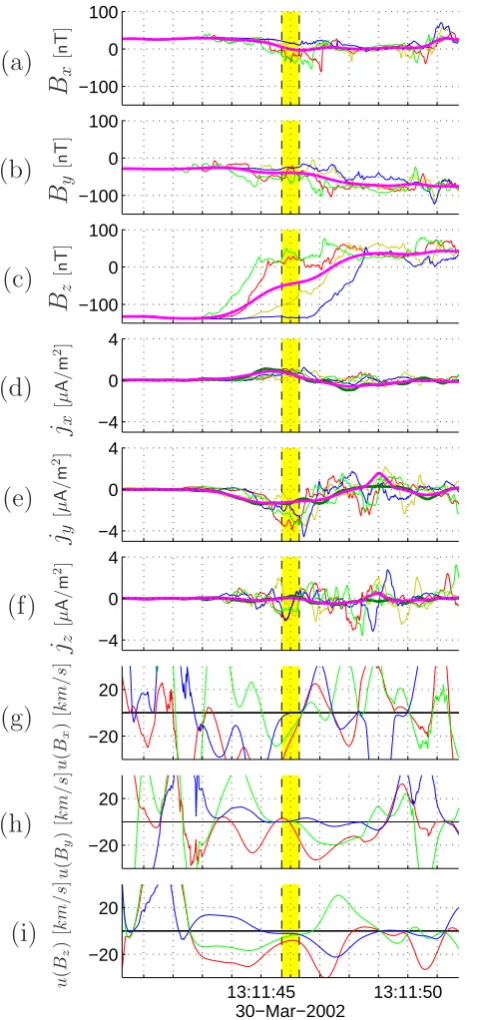
in the GALS least squares problem. The extra information from the included time domain is used to improve the spa-tial resolution. Of course, this requires that the shape of the investigated convective structure is approximately stable on these time scales. In this case, the GALS current will there-fore be more similar to the result from the single-spacecraft method, which is highly capable to resolve small scale struc-tures. In panels (d–f) of Fig. 5 we clearly see that the GALS result rather closely follows the single-spacecraft currents. The curlometer, on the other hand, fails to resolve the small scale variations. Notice that the estimated thickness of the current sheet is about 50 km, which is of the order of the proton gyroradius (in the magnetosheath plasma the gyrora-dius is about 50 km and in the magnetospheric plasma about 25 km).
Panels (i) of Figs. 4 and 5 show the structure velocity obtained in the GALS reconstruction of theBz data which
causes the dominant part of the current sheet. Using a large
coherence time,Tc=6 s as in Fig. 5, we see in panel (i) that
the velocity around the time of the current sheet crossing (about 13:11:46.50) is approximately consistent with the re-sult from the timing analysis, (−23,−11,−4) km/s. On the other hand, using a smallerTc=0.6 s as in Fig. 4, the
veloc-ity estimate in theBz reconstruction does not stabilize on a
specific value during the magnetopause crossing. However, it should be noted that the velocity estimated by GALS is not necessarily closely related to the velocity of a current sheet or some other physical structure in the magnetic field. In many cases it is completely unrelated to the velocity of large scale field structures. As discussed in Sect. 2, the velocity obtained by GALS describes the motion of the frame of ref-erence where the field signal is locally stationary. In that sense, the GALS velocity should rather be regarded as a lo-cal phase velocity than as the velocity of a physilo-cal structure.
[image:5.595.98.495.66.387.2]3496 M. Hamrin et al.: Gradient analysis
8 M. Hamrin et al.: Gradient analysis
−100 0 100 −100 0 100 −100 0 100 −4 0 4 −4 0 4 −4 0 4 −20 20 −20 20 30−Mar−2002
13:11:45 13:11:50 −20 20
B
x [ n T ]B
y [ n T ]B
z [ n T ]j
x [ µ A / m 2]j
y [ µ A / m 2]j
z [ µ A / m 2] u ( Bx ) [ k m / s ] u ( By ) [ k m / s ] u ( Bz ) [ k m / s ](a)
(b)
(c)
(d)
(e)
(f)
(g)
(h)
(i)
Fig. 4. Cluster crossing a thin magnetopause current sheet on March
30, 2002. The colour coding is the same as in Fig. 3. (a)–(c) Mag-netic fieldBx,By, andBzcomponents in the GSE coordinate sys-tem observed by the four spacecraft (red, yellow, blue, green) to-gether with the reconstructed magnetic field from GALS (magenta). (d)–(f) Current density Jx, Jy, and Jz components from GALS (magenta), the curlometer (dark green) and the single-spacecraft method (red, yellow, blue, green). The highlighted time window indicates the used coherence timeTc= 0.6s used in GALS. (g)–(i) The GALS velocityux,uyanduz (red, green and blue) obtained for the magnetic field componentsBx,ByandBz.
−100 0 100 −100 0 100 −100 0 100 −4 0 4 −4 0 4 −4 0 4 −20 20 −20 20 30−Mar−2002
[image:6.595.240.530.58.579.2]13:11:45 13:11:50 −20 20
B
x [ n T ]B
y [ n T ]B
z [ n T ]j
x [ µ A / m 2]j
y [ µ A / m 2]j
z [ µ A / m 2] u ( Bx ) [ k m / s ] u ( By ) [ k m / s ] u ( Bz ) [ k m / s ](a)
(b)
(c)
(d)
(e)
(f)
(g)
(h)
(i)
Fig. 5. Same event and panels as in Fig. 5. The only difference
is that a longer coherence time,Tc, is used in the GALS run. The highlighted time window indicates the used coherence timeTc =
6s.
Fig. 4. Cluster crossing a thin magnetopause current sheet on 30
March 2002. The colour coding is the same as in Fig. 3. (a–c) Mag-netic fieldBx,By, andBzcomponents in the GSE coordinate
sys-tem observed by the four spacecraft (red, yellow, blue, green) to-gether with the reconstructed magnetic field from GALS (magenta).
(d–f) Current density Jx, Jy, and Jz components from GALS
(magenta), the curlometer (dark green) and the single-spacecraft method (red, yellow, blue, green). The highlighted time window in-dicates the used coherence timeTc=0.6 s used in GALS. (g–i) The
GALS velocityux,uyanduz(red, green and blue) obtained for the
magnetic field componentsBx,ByandBz. −100 0 100 −100 0 100 −100 0 100 −4 0 4 −4 0 4 −4 0 4 −20 20 −20 20 30−Mar−2002
13:11:45 13:11:50 −20 20
B
x [ n T ]B
y [ n T ]B
z [ n T ]j
x [ µ A / m 2]j
y [ µ A / m 2]j
z [ µ A / m 2] u ( Bx ) [ k m / s ] u ( By ) [ k m / s ] u ( Bz ) [ k m / s ](a)
(b)
(c)
(d)
(e)
(f)
(g)
(h)
(i)
Fig. 4. Cluster crossing a thin magnetopause current sheet on March
30, 2002. The colour coding is the same as in Fig. 3. (a)–(c) Mag-netic fieldBx,By, andBzcomponents in the GSE coordinate sys-tem observed by the four spacecraft (red, yellow, blue, green) to-gether with the reconstructed magnetic field from GALS (magenta). (d)–(f) Current density Jx, Jy, and Jz components from GALS (magenta), the curlometer (dark green) and the single-spacecraft method (red, yellow, blue, green). The highlighted time window indicates the used coherence timeTc= 0.6s used in GALS. (g)–(i) The GALS velocityux,uyanduz (red, green and blue) obtained for the magnetic field componentsBx,ByandBz.
−100 0 100 −100 0 100 −100 0 100 −4 0 4 −4 0 4 −4 0 4 −20 20 −20 20 30−Mar−2002
13:11:45 13:11:50 −20 20
B
x [ n T ]B
y [ n T ]B
z [ n T ]j
x [ µ A / m 2]j
y [ µ A / m 2]j
z [ µ A / m 2] u ( Bx ) [ k m / s ] u ( By ) [ k m / s ] u ( Bz ) [ k m / s ](a)
(b)
(c)
(d)
(e)
(f)
(g)
(h)
(i)
Fig. 5. Same event and panels as in Fig. 5. The only difference
is that a longer coherence time,Tc, is used in the GALS run. The highlighted time window indicates the used coherence timeTc =
6s.
Fig. 5. Same event and panels as in Fig. 5. The only difference
is that a longer coherence time,Tc, is used in the GALS run. The
highlighted time window indicates the used coherence timeTc=6 s.
4 Summary and discussion
Above we have shown that it is possible to tune GALS to the problem at hand by changing the coherence time,Tc.
Choos-ing a small value of Tc, the current resulting from GALS
[image:6.595.51.293.63.574.2]becomes similar to that from the curlometer while a largerTc
improves the spatial resolution and makes the current more similar to the result from the single-spacecraft method. This demonstrates that GALS is a tool that easily can be applied to large amounts of data and yet provides a resolution com-parable to the single-spacecraft method.
We have applied the GALS method to synthetic magnetic field data and data from the FGM instrument on board the Cluster satellites. The results indicate that GALS is a ro-bust method to obtain high-resolution spatial gradients from multi-spacecraft observations. Furthermore, GALS is sim-ple to use since the user needs to specify only a single pa-rameter, the coherence timeTc. This makes GALS
comple-mentary to the discontinuity analyzer/single-spacecraft tech-nique, which demands substantial user input.
Comparing GALS with the curlometer and the single-spacecraft method, we find that GALS resolves thin current sheets better than the curlometer. GALS can resolve struc-tures on scales considerably smaller than the characteristic size of the satellite configuration, and our tests indicate that it is less sensitive to the spacecraft configuration than the cur-lometer. The single-spacecraft method and GALS provide similar resolutions, but the single-spacecraft method requires a separate calculation of the velocity of the current sheet.
GALS is related to the method of De Keyser et al. (2007) in the sense that they are both based on a weighted least squares fit to the data. However, De Keyser et al. (2007) does not take advantage of the freedom to choose a frame of ref-erence moving with convecting structures in the field. In the absence of coherent convective structures, GALS will com-pute gradients on scale lengths determined by the spacecraft separation, similar to the De Keyser et al. (2007) method. However, when a coherent structure is found, GALS will au-tomatically determine its velocity and produce gradients with resolution similar to the single-spacecraft technique.
Current sheets are important in space physics, since they are ubiquitous at boundaries between plasma populations. Here, we have illustrated the principles behind GALS using current sheets, but it should be clear from the design that nei-ther a current nor a sheet is essential. However, the method requires that the surface of constant F is not too strongly curved within the volume spanned by the spacecraft config-uration. Without this assumption, which is implicit in the curlometer as well as the single-spacecraft methods, it seems impossible to derive meaningful information about gradients. Moreover, GALS requires that the life time of relevant struc-tures in the field is not too short.
We consider our results promising and we expect that the GALS method will be useful when reliable high resolution estimates of spatial gradients are needed. In the future, we intend to develop reliable error estimates, investigate the ca-pacity to separate spatial and temporal variations, and apply the method toN6=4 spacecraft.
Appendix A
The GALS algorithm
A1 Initial setup
Let τn=n1t, n=0,±1, . . . ,±N, be the discrete times at
which the satellites sample the field. At the timeτnsatellite
s is at x0sn=x0s(τn)and observes the fieldFsn=F0(x0sn, τn).
The field sampled by the satellites can be expressed as a Tay-lor expansion
Fsn ≈Fp0+x0sn·∂x0Fp0+τn∂τFp0, (A1)
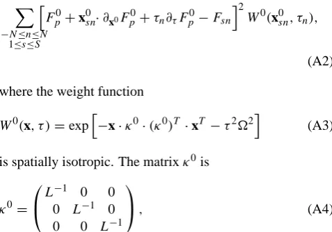
whereFp0and its derivatives at x0=0 andτ=0 are five un-known parameters. The field and its derivatives at the re-construction point are estimated by minimizing the weighted least squares problem
X
−N≤n≤N 1≤s≤S
h
Fp0+x0sn·∂x0Fp0+τn∂τFp0−Fsn
i2
W0(x0sn, τn),
(A2) where the weight function
W0(x, τ )=exph−x·κ0·(κ0)T ·xT −τ22 i
(A3) is spatially isotropic. The matrixκ0is
κ0=
L−1 0 0 0 L−1 0 0 0 L−1
, (A4)
whereLis the characteristic size of the spacecraft configu-ration (Paschmann and Daly, 1998) and=1/Tc. The
co-herence timeTc is a user-defined parameter that designates
[image:7.595.308.547.281.448.2]the time scale during which the local structure of the field is expected to retain its approximate shape.
Figure 1a illustrates the sampling of the field in the satel-lites frame of reference. The spatial coordinates x0sn of the satellites are essentially independent of n (i.e., time), and take on only four distinct values. Although the spatial res-olution will be as low as if we used only one observation per spacecraft, minimizing Eq. (A2) will give us a first estimate of Fp0,∂x0Fp0, and ∂τFp0. These estimates can then be
im-proved by iteration.
A2 Iterative improvements
velocity we introduce fori≥1 a unit vectoruˆi parallel to the
estimated spatial gradient,
ˆ
ui = ∂xi−1F
i−1 p ∂xi−1F
i−1 p
, (A5)
Assumingu0=0, the velocity, relative to the satellites, of the field structure at the reconstruction point is then determined as
ui =
ui
−1·uˆi − ∂τF i−1 p ∂xi−1F
i−1 p
uˆi. (A6)
The velocity ui describes how a plane, tangent to a surface of constantF at(rp, tp), moves along the gradient. In some
simple cases, such as the magnetic field generated by a con-vecting plane current sheet, ui will be closely related to the velocity of the current sheet. However, in more complicated situations ui may be completely unrelated to the motion of large scale field structures. Notice that ui should not be
inter-preted as the velocity of a physical object, but is more similar to a locally defined phase velocity.
To improve the resolution, an anisotropic weight function is used in the iterations. Introduce two orthogonal unit vec-torsvˆi andwˆiin the plane perpendicular touˆi. In this plane
the field will be slowly varying, and a resolution∼Lis ac-ceptable. To resolve the gradient as well as possible we focus on measurements taken close to this plane through the origin and within the coherence time (|τn|.Tc/2). Hence, we
de-fine the weight functionWias
Wi(x, τ )=exph−x·κi·(κi)T ·xT −τ22 i
(A7) where
κi = uˆi
3i,
ˆ vi
L,
ˆ wi
L
. (A8)
The resolution3i is mainly determined by the magnitude of the velocityui=|ui|of the satellites in the structure’s frame of reference. As illustrated in Fig. 1b, consecutive obser-vations from each satellite will be separated by a distance 1t >ui in the direction of the gradient. Thus we can typ-ically choose 3i∼1t >uiL and still have measurements with significant weight from all spacecraft. However, if the velocity is low or the coherence time short, so thatTc>ui<L,
the algorithm will increase3i in order to include data from all satellites.
A3 The algorithm
After obtaining the initial estimates according to Eq. (A2– A4), the GALS algorithm can be summarized as follows: For i=1,2, . . .
I. Transform to the frame of reference moving with veloc-ity uiby defining
xi =x0−τui, Fi(xi, τ )=F0(xi+τui, τ ). (A9) II. Solve the weighted least squares problem
X
n,s h
Fpi +xisn·∂xiFpi +τn∂τFpi −Fsn i2
Wi(xisn, τn)
(A10) to obtain estimates of∂xiFpi and∂τFpi in this reference
frame.
III. Calculate a refined velocity estimate according to Eq. (A6).
These calculations are repeated until the velocity update falls below a threshold. The final results are then transformed back to the initial frame of reference according to
∂rF =∂xiFi, ∂tF =∂τFi−(Prp+ui)·∂xiFi. (A11) The GALS algorithm is applied to each timestep indepen-dently. For the case of magnetic field observations, GALS treats each component,Bx,By, andBz, and it obtains
esti-mates of the velocity u and resolution3along the spacecraft orbit for structures in each field component. However, the three field components are coupled together with an addi-tional constraint in our least squares routines by the use the Maxwell equation∇·B=0.
Acknowledgements. We acknowledge S. Buchert for help with
FGM data and J. De Keyser for fruitful discussions.
Topical Editor I. A. Daglis thanks J. De Keyser and U. Motschmann for their help in evaluating this paper.
References
Balogh, A., Dunlop, M. W., Cowley, S. W. H., et al.: The Cluster magnetic field investigation, Space Sci. Rev., 79(1–2), 65–91, doi:10.1023/A:1004970907748, 1997.
De Keyser, J., Dunlop, M. W., Darrouzet, F., and D´ecr´eau, P. M. E.: Least-squares gradient calculation from multi-point observations of scalar and vector fields: Methodology and applications with Cluster in the plasmasphere, Ann. Geophys., 25, 971–987, 2007, http://www.ann-geophys.net/25/971/2007/.
De Keyser, J., Dunlop, M. W., Owen, C. J., Sonnerup, B. U. ¨O., Haaland, S. E., Vaivads, A., Paschmann, G., Lundin, R., and Rezeau, L.: Magnetopause and boundary layer, Space Sci. Rev., 118, 231–320, 2005.
Dunlop, M. W. and Woodward, T.: Multi-spacecraft Discontinu-itu Analysis: Orientation and Motion, in: Analysis methods for multi-spacecraft data, edited by: Paschmann, G. and Daly, P. W., 271–305, ISSI Scientific Report SR-001, 1998.
Dunlop, M. W., Balogh, A., Glassmeier, K.-H., and Robert, P.: Four-point cluster application of magnetic field analysis tools: The Curlometer, J. Geophys. Res., 107(A11), 1385, doi:10.1029/ 2001JA005089, 2002.
L¨uhr, H., Warnecke, J. F., and Rother, M. K. A.: An algorithm for estimating field-aligned currents from single spacecraft magnetic field measurements: A diagnostic tool applied to Freja satellite data, IEEE Trans. Geosci. Remote Sens., 34, 1369–1376, 1996. Panov. E. W., B¨uchner, J., Fr¨ana, M., Korth, A., Khotyaintsev,
Y., Nikutowski, B., Savin, S., Fornac¸on, K.-H., Dandouras, I., and R`eme, H.: CLUSTER spacecraft observation of a thin cur-rent sheet at the Earth’s magnetopause, Adv. Space Res., 37, 1363–1372, doi:10.1016/j.asr.2005.08.024, 2006.
Robert, P., Dunlop, M. W., Roux, A., and Chanteur, G.: Accuracy of Current Density Detrmination, in: Analysis methods for multi-spacecraft data, edited by: Paschmann, G. and Daly, P. W., 395– 418, ISSI Scientific Report SR-001, 1998.