Summer planetary-scale oscillations: aura MLS temperature compared with ground-based radar wind

www.ann-geophys.net/27/1763/2009/

© Author(s) 2009. This work is distributed under the Creative Commons Attribution 3.0 License.

Annales

Geophysicae

Summer planetary-scale oscillations: aura MLS temperature

compared with ground-based radar wind

C. E. Meek and A. H. Manson

Institute of Space and Atmospheric Studies, University of Saskatchewan, Saskatoon, S7N 5E2, Canada Received: 8 December 2008 – Revised: 9 March 2009 – Accepted: 2 April 2009 – Published: 9 April 2009

Abstract. The advent of satellite based sampling brings with it the opportunity to examine virtually any part of the globe. Aura MLS mesospheric temperature data are analysed in a wavelet format for easy identification of possible planetary waves (PW) and aliases masquerading as PW. A calendar year, 2005, of eastward, stationary, and westward waves at a selected latitude is shown in separate panels for wave num-ber range−3 to +3 for period range 8 h to 30 days (d). Such a wavelet analysis is made possible by Aura’s continuous sam-pling at all latitudes 82◦S–82◦N. The data presentation is suitable for examination of years of data. However this pa-per focuses on the striking feature of a “dish-shaped” uppa-per limit to periods near 2 d in mid-summer, with longer periods appearing towards spring and fall, a feature also commonly seen in radar winds. The most probable cause is suggested to be filtering by the summer jet at 70–80 km, the latter be-ing available from ground based medium frequency radar (MFR). Classically, the phase velocity of a wave must be greater than that of the jet in order to propagate through it. As an attempt to directly relate satellite and ground based sam-pling, a PW event of period 8d and wave number 2, which appears to be the original rather than an alias, is compared with ground based radar wind data. An appendix discusses characteristics of satellite data aliases with regard to their pe-riods and amplitudes.

Keywords. Atmospheric composition and structure (Instru-ments and techniques) – Meteorology and atmospheric dy-namics (Middle atmosphere dydy-namics)

Correspondence to: C. E. Meek

([email protected])

1 Introduction

Many papers have been written in the past, and continue to be written, describing attempts to obtain characteristics of mesospheric planetary waves from a few isolated ground-based sites (Meek et al., 1996; Luo et al., 2002). Satellites now provide vast improvement in spatial sampling, but at the expense of temporal sampling. Though there have been a few satellites devoted to sampling upper atmospheric winds, e.g. UARS (Upper Atmosphere Research Satellite) and TIMED (Thermosphere Ionosphere Mesosphere Energetics and Dy-namics), they have not replaced ground based sampling. On the other hand, temperature is commonly measured by satel-lites, e.g. Aura MLS (Mesosphere Limb Sounder), SABER (Sounding of the Atmosphere using Broadband Emission Ra-diometry) and others. A combination of satellite tempera-tures and ground based wind data may help to solve some temporal ambiguities (aliasing) in the former and spatial am-biguities due to sparse sampling in the latter.

Wavelet analysis is a convenient way to identify planetary wave events. Here, as in Manson et al. (2004a), the data are separated by wavenumber into apparent eastward, station-ary, and westward propagating waves. As with any regularly sampled data, the potential for aliasing must be considered. Thus the frequency range is extended beyond the Nyquist pe-riod (which is 2 d here if single node sampling at a fixed loca-tion is considered) into the tidal period range, where globally coherent waves are also expected.

In the course of this work, a “dish shaped” feature was noted in PW frequency, an apparent frequency limit which increases from spring to mid summer (at which time the pe-riod is near 2 d) and decreases towards fall, when slower waves, longer periods, are again seen. This feature has long been noted in radar data as well. It is suggested that it is due to filtering by the lower mesosphere zonal wind.

High inclination orbit satellites have slow or no (“sun syn-chronous”) precession in local time - basically the Earth turns under a completely or almost completely stationary or-bit. The Aura satellite is sun synchronous,∼90 min orbital period, with sampling 82◦S to 82◦N. We use level 2, ver-sion 1.5x, data here. Data are gridded in 121 latitude bins, approxmately 0.5 to 1◦_{steps depending on latitude, and 37} pressure levels, approximately 3 to 6 km steps depending on height. The line of sight is along the orbit, so the full latitude range is sampled all year. The stated orbital period means that tracks are spaced about 24◦in longitude at any latitude. As radar scientists we are used to thinking in terms of geo-metric height rather than pressure, so we translate the latter to approximate height by h(km)=(64.8/4.)(3.-log10P(mb)) in

figure labels. At 90 km, the averaging interval is about 15 km (Schwartz et al., 2008). Planetary waves usually have much longer vertical wavelengths, but we cannot rule out some mi-nor reduction in amplitude due to height averaging.

The wind data are from MF radars located near Saskatoon (52◦N, 107◦W), Platteville(40◦N, 105◦W), and Tromsø (70◦N, 19◦E) which operate continuously (e.g. Manson et al., 2003; Hall et al., 2003)).

3 Analysis

At a fixed height and latitude, a zonally propagating plane-tary wave is assumed to have the form

v=Vcos(ωt+m`−φ) (1) wherevis the measured parameter,V is the wave amplitude,

ω is the wave frequency, mis the wavenumber, t is time, and`is the East longitude (radians). The phase φ can be interpreted as the time of maximum at zero longitude, or as the position of maximum (given by longitude =φ/m) at zero time.

Unlike satellites such as EP TOMS (Total Ozone Measur-ing System), the Aura MLS makes limb measurements on both ascending and descending nodes. Solar tides are ex-pected to be significant at the upper mesospheric heights, and

comprisenAandnDsamples respectively) as 2Wcorr

q

X2_R+X2_I

where

XR = 1 2    1 nA tA2

X

tA=tA₁

W (TA−TA)cos(ωtA+m`A)

+ 1

nD tD2

X

tD=tD₁

W (TD−TD)cos(ωtD+m`D)  

 (2)

XI = 1 2    1 nA tA₂ X

tA=tA1

W (TA−TA)sin(ωtA+m`A)

+ 1

nD tD₂ X

tD=tD1

W (TD−TD)sin(ωtD+m`D)  



. (3)

This has the form of added A and D Fourier Transforms (FT, but at one frequency) whereW represents a truncated Gaussian window, amplitude 1.0 (centre) to 0.05 (ends), and

Wcorr=2 is the window correction factor. An advantage of

the FT method over a least squares fit is that the resulting amplitudes are limited by the measured values. In the the-oretical case of a single wave, both methods give the same result.

For each frequency the window length is arbitrarily cho-sen to be 6 times the period. The frequency range for the plot is divided into 600 pixels (logarithmic range covering peri-ods 8 h–720 h), and interval time (one year) into 800 pixels. There is no smoothing other than that inherent in the over-lapping times and bandwidths of the windows.

but here the plotted frequency range has been extended to much shorter periods in order to reveal, for example, non-migrating tides (Meyer and Forbes, 1997) or their non-linear interaction byproducts, whose aliases might be mistaken for the long period waves of interest.

A log amplitude scale is used, “dB”=20 log₁₀T, whereT

is in K◦, to enhance the appearance of the smaller oscillations at the expense of the larger, and the “gain” is also increased with spatial wavenumber since power tends to be related to geophysical spatial scales. For example “+3 dB’ indicates an amplitude gain of

√

2, “+6 dB” an amplitude gain of 2 etc. These act to bring weaker features into view. In addition data are clipped above a certain value - usually these extreme values occur at 24 or 12 h (which are aliases for stationary waves, as will be shown later).

Log frequency is a convenient way to expand the low fre-quency range. Both this and the log amplitude scales are helpful for a quick look but are somewhat detrimental when it comes to detecting aliases.

Figure 1 shows a wavelet plot for 2005, 51◦N, 91 km. Three “cycles” are shown: infinity-24 h, 24–12 h, 12–8 h. As will be discussed in the next section, a peak in one cycle will appear again in this cycle as an alias and twice in each of the other two, but at different wavenumbers and usually with reduced amplitude.

A few comments on the high frequency (tidal) periods are pertinent here. Considering that the migrating tides should have been mostly removed, as evidenced by the null right at 24 and 12 h for wavenumbers +1 and +2, respectively, it is not clear why the features near 24 and 12 h are so strong. If increasing significance criteria similar to that of Scargle (1982) are applied, a limit based on the ratio of spectral power at one frequency to total power, these are the last to survive. There are several possible reasons: (1) Amplitude modulation of tides, e.g. by transient PW, will have side-bands, not exactly at 24/12 h, which will remain; (2) Non-migrating tides (NMT) are a possibility, but by definition these have different wavenumbers than the respective migrat-ing, so the 12 h,m=+1 and 24 h, m=+2 are possible exam-ples; (3) Because zero frequency is aliased to 24 and 12 h, long term trends will also contribute, (4) The absolute band-width of a Fourier bin, 1/τ, for a short sequence lengthτ is wider than for a long and so the shorter sequence has more background noise per bin, or put another way: the original variance is divided between Fourier bins so the fewer the number of bins, the more power each has. Further analy-ses with constant length sequences for all frequencies, linear frequency scales etc. (not shown) have suggested tidal mod-ulation and aliases of very low frequencies and/or trends as the most probable cause.

The over-plotted line is calculated from Saskatoon peak zonal hourly wind near local noon (18:00–19:59 UT) in the height range 55–79 km (see Fig. 2). These daily values form a sequence which is averaged in parallel with the wavelet analysis, using the same frequency-dependent window and

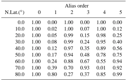
Table 1. Amplitudes of aliases for orbit tilt = 8◦, ts=1 d,

torb=91.6791 min versus latitude.

Alias order

N.Lat.(◦) 0 1 2 3 4 5

0.0 1.00 0.00 1.00 0.00 1.00 0.00 10.0 1.00 0.02 1.00 0.07 1.00 0.12 20.0 1.00 0.05 0.99 0.15 0.98 0.25 30.0 1.00 0.08 0.99 0.24 0.95 0.40 40.0 1.00 0.12 0.97 0.35 0.89 0.56 50.0 1.00 0.17 0.94 0.48 0.78 0.75 60.0 1.00 0.24 0.88 0.67 0.55 0.94 70.0 1.00 0.39 0.70 0.93 0.01 0.92 80.0 1.00 0.80 0.27 0.37 0.85 0.99

correction factor that was applied to temperature. Finally this average wind speed and the global wavenumber for the plot, are converted to a frequency. That is, a wave of this fre-quency and wavenumber will have a (westward) phase speed equal to the radar wind. A black dot is placed in the plot if this frequency, converted to a frequency pixel index, coin-cides with that of the row being plotted.

4 Aliasing

Before we can have confidence that we are looking at a PW signature, we must make sure it is not just an alias of a higher frequency event. Salby (1982) has given a very mathemati-cal description of aliasing in satellite data analysis. In the appendix we present what seems to us a simpler derivation, leading to the results we need. These are the following. If an actual wave has wavenumberm1and frequencyf1then its

aliases arem,f, given by

m=m1+n, and

f fs

=f1

fs

+n (4)

wherefs is 1/tswheretsis the time for the satellite to cover all longitudes (e.g. 1 d for Aura),m, m1must be integers, and

n=0,±1,±2,±3 ...

The amplitude of an alias is given by

VA&D =V0cos

n

21L (5)

whereV0is the amplitude of the actual wave (n=0), n is the

“alias order”: 0,±1,±2, ..., and1Lis the azimuthal angle between ascending (A) and descending (D) node samples at the same latitude in the sun synchronous reference system.

Table 1 shows some values for a satellite with sampling parameters similar to Aura. SABER is somewhat different in that it looks perpendicular to its orbit path, and changes sides every 2 months, so as not to be looking towards the sun. Since the sampled path is not an earth-centred circle,

Fig. 2. Daily noon zonal wind at Saskatoon.

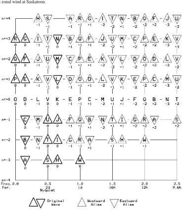
Fig. 3. Chart of aliases for a selection of original waves (see text for full explanation).

For long term intervals it must also be taken into account that SABER precesses 3◦ per day eastward (i.e. faster than the earth turns), sots=360/363 d.

Figure 3 is a chart of original waves and some of their aliases (from Eq. 4). An alphabetic character surrounded by a heavy triangle is the original wave; the same character in

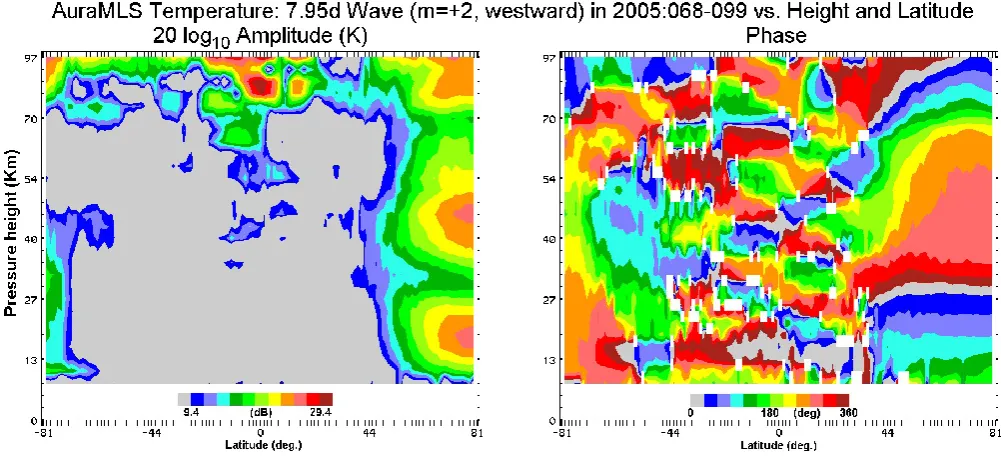
Fig. 4. Spring 2005 oscillation in temperature of period 7.95 d, wave number +2: amplitude and phase values the Aura MLS. Data latitude

range is:−82 S to 82 N.

“distance” between aliases for the purpose of finding relative amplitudes (viz. if one of aliases is considered to be the real wave). The frequency scale is in cycles perts. In the period scaled should be replaced byts for non-solar synchronous satellites. Of particular interest in winter are stationary wave aliases: for example wave 1 has an weak alias atm=2, 24 h at our latitude, and a strong one atm=3, 12 h, among others (see Eq. 4, Table 1, and Fig. 1).

The foregoing model has assumed stationarity. In the real world wave events will have lifetimes. The wavelet plot is suited to this, but can be misleading while looking for aliases since a short burst at short period is not likely to lead to a long period alias, and also amplitudes, real or aliased, depend on the length of the real event relative to the window as well as on the alias order. This complicates matters considerably, to say the least.

On the other hand, near the poles, the satellite is moving fast in longitude and local time (the maximum speed is about 2 LT h, or 30 degrees of longitude, per minute), and some po-tential aliases may be averaged out by the effective sampling window, 1–2 min.

4.1 Discussion of aliases in relation to the measure-ments

As stated previously the “noise” level is expected to be higher at the higher frequencies because of the wider bandwidth for short sequences. This is likely obscuring many of expected aliases, but with reference to Fig. 1, the peak atm=−1, period T∼5 d, near day 31 would be like “C” in Fig. 3 We expect to see it also at a period between 24 h and 2 d atm=+2, and

there is a small feature there. The featurem=3,T∼5 d near day 345, like “G” in Fig. 3, should have an alias atm=−2 between 24 h and 2 d. It does, and is stronger so we have to rule out them=3 peak. There is also is a third possibility at

m=−1.

5 Selected PW, wave numberm=2, periodT=7.95 d

The apparent planetary wave in Fig. 1, day∼91, atm=+2, periodT of 7.95 d has been chosen for detailed analysis. Ac-cording to Fig. 3 (wave “F”) its nearest alias should be at

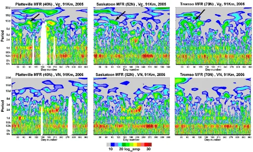
Fig. 5. Wavelets of zonal radar winds for 2005 at 91 km for Platteville (40◦N, 105◦W), Saskatoon(52◦N, 107◦W), and Tromsø (70◦N, 19◦E). Overplotted arrows show where the 8d wave should appear. The colour scale is dB (20 log₁₀Amp ). Meridional wind wavelets for 2006 are included.

is correct or just an alias of a higher frequency event. In this case we just have wind data, but since planetary waves affect both wind and temperature, the effort is still worthwhile, al-though the global PW structure could be such that the wind and temperature amplitudes peak at different latitudes. The latter appears to be the case for the three radar sites shown in Fig. 5, in which the selected wave in the east-west wind component is strongest at Platteville, weak at Saskatoon, and not present at 7.95 d at Tromsø. Regarding the latter site, however, there is a peak near 7 d that could be a local man-ifestation of the 8d wave of interest. The studies of Luo et al. (2002) show such changes in observed PW periods from Tromsø to Christmas Island, and discuss these in terms of possible Doppler shifting and/or changing resonance condi-tions in different hemispheric locacondi-tions.

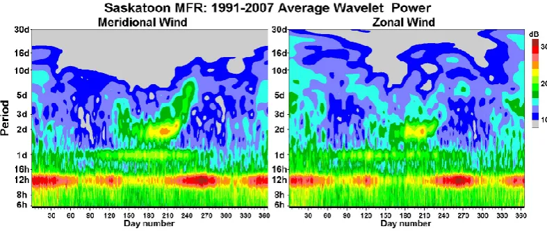
6 Summer frequency “dish”

We now return to the feature that was the main instiga-tor for this study, the summer “dish” shape of amplitudes in frequency-time spectra seen in both satellite temperature (Fig. 1) and ground based radar winds. Though the latter is not clearly seen in the zonal wavelets for 2005 in Fig. 5, it is

Fig. 6. A 17 year (1991–2007) average wavelet power plot for Saskatoon radar wind at 91 km, meridional and zonal components.

in Fig. 1. It is a close but not a perfect match to the dish. One reason is that although the waves are from global temperature data, the calculated phase speed limit imposed by the zonal wind jet is based on one site (using maximum daily noon wind in the height range 58–79 km, which had then been av-eraged over the same window as used in the wavelet calcula-tion). Some waves in Fig. 1 are seen at 92 km, particularly atm=+3 but alsom=+1 and +2, which according to theory should not have penetrated this jet. Notice again however the PW of longer period, viz. lower phase speed, further from the overplotted limit line, are excluded. It is possible that the wind value is biased because of tidal contamination, or be-cause a single site cannot properly represent the global zonal wind.

Monthly fits of mean plus tides (24 h, 12 h) were applied to Saskatoon radar data and showed that tidal contribution to the noon zonal values is of the order of 5–10 m/s at 79 km, and is usually positive. That is, the noon wind is more westward than the daily mean. However at lower heights, say 70 km, where the wind can be strongest, the tidal contamination is smaller, and sometimes negative. There is also the issue as to the duration of any regime in background winds: this should be for at least as long as the range of PW periods in question. More important is the variation of zonal wind with longi-tude. There appears to be a significant standing wave in sum-mer. Reference to UKMO/MetO assimilated model winds at the 0.3 mb level (circa∼56 km) shows that in 2005 the average July zonal wind speed has its maximum at 300◦_E (U=−61 m/s) and minimum at 130◦_{E (U=−42 m/s). A} sim-ilar pattern was found in the two other years checked, 2003 and 2004, but it had slightly reduced maxima. That is, Saskatoon zonal winds are stronger than the global mean. If this pattern continues up to the jet maximum it could help to explain how some waves do not experience critical lev-els near 70 km. For example in 2005 (Fig. 1), the maxi-mum mid-summer (windowed) radar wind value used was 84 m/s, equivalent to a limiting period of 1.13 d (atm=+3,

and 51.7◦N). If we scale by the MetO value ratio, on the as-sumption that some fraction of the wave energy can penetrate at the weakest wind location, the limit would be 1.64 d.

An alternate explanation, suggested by a reviewer, is that gravity waves modulated by lower stratosphere wind might pass through the jet and deposit their energy at greater heights, thus re-generating the PW. This method was pro-posed by Smith (2003) for producing stationary planetary waves in the upper mesosphere.

It is interesting that the modulation in the mid-summer quasi two day temperature wave (Q2DTW), in them=+3 sec-tor of Fig. 1, in mid summer is similar to the modulation of the zonal wind.

The appearance depends partly upon the windowing, which is the same for both, but the impression is that the Q2DTW is absent for the strongest winds – that is for pe-riods above the two lowest values of the overplotted phase speed limit. This result is consistent with the westward phase velocity being then consistently lower than the background wind and hence the occurrence of critical levels. More gener-ally, the monthly occurrences of the Q2DW atm=+3, which include winter as well as summer months, are very consis-tent with the radar-wind studies of this wave (Meek et al., 1996; Chshyolkova et al., 2005). We also note that although the non-linear interaction between the Q2DW and the diur-nal tide has been documented for particular events (Manson et al., 1998; Pancheva, 2006), instances of the production of 16 h oscillations are not numerous enough to lead to a spec-tral peak in Fig. 6.

However for SABER at 45◦_{S in the late January yaw} con-figuration (maximum southern latitude sampled is∼50◦_S), the A and D samples are quite close together in longitude, and so the alias should be strong, similar to Aura at 80◦N. On the other hand, SABER’s slow precession may have to be taken into account.

7 PW wave number spectra and the “best mode”

Firstly, a few general comments on Fig. 1 (and indeed Figs. 4 and 5) are appropriate. The dominance of periodsT near 5, 10 and 16 d and with wave numberm=+1 during months with eastward background winds is consistent with radar wind studies by Luo et al. (2002) and others: these are the so-called Rossby Waves. Other studies have noted oscillations in the temperature field with periods near 5 days andm=+1 during summer months at high latitudes (Kirkwood et al., 2002). There has been little discussion in the literature of ob-served PW withm<0, consistent with the smaller intensities of those wave numbers in Fig. 1, and the theoretical require-ment for PW to have phase velocities that are westward with respect to the background wind (Andrews and Holton, 1987). There is another limit associated with the propagation of PW into the middle atmosphere: the difference between the background wind and the PW phase speed (allowing for sign) shall be less that a so-called “critical velocity”Uc (Charney and Drazin, 1961; Andrews and Holton, 1987; Manson et al., 2005). Thus in the winter months the Rossby Waves will propagate vertically more strongly when the eastward winds (westerlies) are weaker e.g. during the major stratospheric warmings, than when the winds associated with the winter polar vortex are at their maximum. Consistent with this, in Fig. 1 form=+1, winter-PW with periods of less than 5 days that would have large phase speeds, are seldom in evidence (usually excluded); while oscillations of these periods are more evident atm=+2 and 3. This is particularly clear for the PW of period near 2 days andm=+3, which is the win-ter manifestation of the Rossby-gravity wave Q2DW. As dis-cussed elsewhere (Nozawa et al., 2003; Chshyolkova et al., 2005) these waves had not been considered until recently, due to the radar-types used and emphasis upon the Summer Polar Mesospheric Echoes (PMSE) in the Scandinavian sec-tor.

We return to Fig. 1: which spectral peaks represent ac-tual PWs and which are their aliases? Since these latter will show generally smaller amplitudes, never bigger than the ac-tual wave, one way to select is by amplitude. To do this we will borrow an idea from Manson et al. (2004a): different modes are coded with different colours, and the mode with maximum amplitude is plotted.

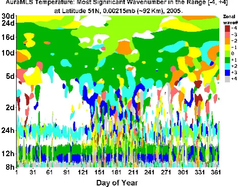
However not everything is a PW, so we would like to ap-ply a criterion for significance. An argument that has been used by Scargle (1982) is as follows. Consider a white noise data sequence ofν equi-spaced points with variance

Fig. 7. A wavelet-format plot based on the analysis used in Fig. 1,

but showing the wave number in the range−4 to +4 with greatest significance at each frequency/time.

σ2. The expected power in a single spectral bin is then

Pav=σ2/νbecause power is equally distributed over all fre-qency bins, and the power in any bin f relative to the expected isz=P (f )/Pav.

The Scargle assmption is that the white noise is such that z has an exponential distribution, viz. the probability of find-ing a value ofzbetweenzandz+dz ise−z. Therefore the probability of findingz<zc in noise is(1−e−zc). The cor-responding signifiance level, viz. the percentage probability that the signal is not noise, is 100(1−[1−e−zc]).

The second argument used is that if a spectrum with µ

independent frequencies is examined, there are more chances to findz>zcin white noise, and therefore the probability of

z<zcis reduced to(1−e−zc)µ. Thus more cases ofz>zcare expected, and the percentage significance level, that is the probability ofz<zcis reduced to 100(1−[1−e−zc]µ).

In relation to the present analysis, it seems thatµ is al-ways one since, with a sequence 6 times the period, we are only looking at one frequency. However when the frequency-time plot is considered as a whole, the arguments aboutµare more difficult. For the present we will useµ=1 and apply a somewhat arbitrary significance level. zcwill be the ratio of individual frequency power to the part of the total sequence variance we would expect to find at that frequency if the data were pink noise with a log-frequency log-power slope of−1 to−2. (The actual % level used was arbitrarily chosen to clear out some of the weaker areas of the next figure, 7.) As mentioned before, if we use this significance scheme and in-crease the level, the last remaining data are at 12 and 24 h.

This concern regarding Fig. 7 is similar to that discussed in Sect. 6 with regard to Fig. 1, where it was noted that the longitudinal maximum zonal wind could be lower than that used to produce the over-plotted line representing the criti-cal level for the PW oscillations. There it was noted that the zonal mean speeds could well be less than at Saskatoon, and hence the over-plotted line could be located at periods during mid summer which are somewhat low. Alternate possibili-ties are some PW leakage or penetration at the critical level; that there is atmospheric resonance at these preferred Rossby wave spatial and temporal scales; that PW of these periods, viz. waves with low frequency and higher wave number, do not exist; or as a refereee has suggested, that they may have propagated from the other hemisphere.

Certainly, and in summary, it is the case that Rossby waves of periods near 10 and 16 days are rationally excluded from the summer atmosphere using the critical level argument and the associated over-plotted line; that the preferred/dominant wave number for PW of periods equal to or greater than 5 days is m=1; that PW periods between 2 and 5 days are dom-inantlym=+2, and that for the Q2DTWm=+3 is statistically favoured in the temperature field at middle latitudes.

8 Summary and conclusions

We have shown that the likely explanation for the “dish” shape in summer-centred frequency-time spectra at mid-latitude is that planetary waves (PW) with sources in the lower atmosphere propagate into the mesosphere during the winter and neighboring equinoctial months, but that systematically those with phase speeds lower than that of the summer-like zonal stratospheric-mesospheric jet at 50– 80 km, are filtered out or blocked from entering the upper mesosphere. The “critical level” overplotted on Fig. 1, where the PW zonal phase speed matches the background flow, has a seasonal variation in the spring and fall months that par-allels that of the reduction of PW activity with long periods (10–16 days). These long periods dominate the winter cen-tred months of the upper mesosphere, when a similar phase speed limit does not exist. In the middle of summer the

re-was seen increasing in amplitude and stable in phase from 45 to 82◦_{N, but in wind measurements the strongest} mani-festation was at Platteville (40◦_{N). It was weaker at} Saska-toon (52◦_{N) and not seen at all, or overshadowed by local} effects, at Tromsø (70◦N). Such latitudinal variations are not unusual, given the observations of the 5 d period PW in the temperature field of northern Scandinavia, and its relative ab-sence at middle latitudes such as Saskatoon.

Appendix A

In the following identification of aliases we will assume reg-ular sampling – viz. constant time/longitude steps at any lat-itude. We do not consider wavenumber aliases, which for Aura implies wavenumbers greater than 7, on the argument that such a small spatial feature unlikely to be globally co-herent. A simple place to start is one-node sampling; e.g. the EP TOMS satellite, where sample longitude is directly related to sample time. However we will not necessarily as-sume sun synchronicity as we do for TOMS or Aura. Time

ts will denote the time for the satellite to cover all longitudes (frequencyfs) andtorb the time for an orbit. For example

Aura has ts=1 d and torb∼90 min. The (temporal) Nyquist

frequency for single node sampling isfs/2. This is easy to see if it is imagined that orbital period is such that the same longitudes are sampled each day.

As in Eq. (1) a specific planetary wave at a given latitude and height in some parameter,v, can be written

v=V0cos(ω1t+m1`−φ1) (A1)

The sample timestare discrete and equi-spaced and the sam-ple longitudes are related to them by`=−2π t /tsplus a con-stant ( the earth is turning “Eastward” under the satellite)

The result of a “FT” at an arbitrarily chosen frequencyf

and wavenumbermis

XR = 1

n

n X

1

{V0cos(ω1t+m1`−φ1)cos(ωt+m`)} (A2)

= 1

n

n X

1

+V0sinφ1sin(ω1t+m1`)cos(ωt+m`)} (A3)

XI = 1

n

n X

1

{V0cos(ω1t+m1`−φ1)sin(ωt+m`)} (A4)

= 1

n

n X

1

{V0cosφ1cos(ω1t+m1`)sin(ωt+m`)

+V0sinφ1sin(ω1t+m1`)sin(ωt+m`)} (A5)

For XR or XI to have a non zero result, cosxcosy or sinxsiny must havex=y orx=y±π, and sinxcosy must have x=y±π/4 (thus converting at least one product to ±sin sin or±cos cos).

Any non zero average in this “monochromatic”, infinite data length, case represents an alias; so a real wave with pa-rametersω1, m1has aliases given by:

ω1t+m1`=ωt+m`±nπ/4 (A6)

wheremmust be an integer, and n=0, 1, ... because each case results in at least one sin sin or cos cos term. However in practice the additional phase term,ϕ=nπ/4 can be shown to be zero as follows. In

ω1t+m1`=ωt+m`+ϕ (A7)

we know that in sampling at one latitude circle`andt are related by`=−2π t /ts. This means that ϕ must also be a function oft, therefore the only constant it can be is zero.

So finally the only aliases tom1, f1are

m=m1+n,

f fs

= f1

fs

+n (A8)

wherem, m1must be integers, andn=0,±1,±2,±3 ...

When only one node is used, all aliases have the same am-plitude.

Two node sampling is a more interesting case. Each node has the same alias frequencies, because the sampling is equivalent except for a constant longitude offset, but po-tentially different phases for the A and D aliases, which may result in some cancellation. The Nyquist remainsfs/2 for each node.

Let the time and longitude for ascending node samples be

tAand`A, and for descending node be,tDand`D. Then

vA=V0cos(w1tA+m1`A−φA) (A9) and

vD=V0cos(w1tD+m1`D−φD) (A10) For a fixed latitude,tA−tD and`A−`D are constants. The spacing between `A and`D will vary with latitude, being close to π at the equator (the earth has turned by π t /torb

radians between samples at the equator) and 0 at the North or South-most sample point. This can be calculated from the

tilt of the orbit,γ, and the latitude,α. The two sample points are spaced by an “azimuth” angle

1L=2 cos−1(tanαtanγ ) (A11)

radians in “longitude”, but since the samples aren’t simulta-neous, and the earth has rotated somewhat between samples, this is not the difference in longitude between samples (un-less it is imagined that the earth is not rotating.)

Therefore the result of using A and D data (with the FT analysis) is equivalent to adding the wave vectors for A and D;V0will be the same for separate A and D aliases but the

A and D phase difference effects some cancellation. Amp=

q

(V0cosφA+V0cosφD)2+(V0sinφA+V0sinφD)2 (A12) For the “real” wave,φA=φD, so the correct amplitude is ob-tained. If these phases are not equal some, or maybe major, cancellation will result. It can be shown that the wave ampli-tude is given by:

VA&D =V0cos

n

21L (A13)

whereV0is the amplitude of the actual wave (n=0) andnis

the “alias order”: 0,±1,±2, .... A (pleasant) surprise is that there is no dependence on real wave mode or frequency, just on the order of the alias.

Acknowledgements. The authors are grateful to the Jet Propulsion

Lab (JPL) for access to the Aura MLS data. Due to superior archiv-ing, it is very nice data to work with! We are also grateful to the British Atmospheric Data Centre (BADC) for the stratospheric as-similated model (UKMO/METO), to the Institute of Space and At-mospheric studies, through the University of Saskatchewan, for re-search facilities, and to Canada’s National Sciences and Engineer-ing Research Council (NSERC) for financial support through a Dis-covery Grant. We appreciate the careful assessment and suggestions by the two reviewers.

Topical Editor C. Jacobi thanks two anonymous referees for their help in evaluating this paper.

References

Andrews D. G., Holton, J. R., and Leovy, C. B.: Middle At-mosphere Dynamics, Academic Press (San Diego), pp. xi+489, 1987.

Charney, J. G. and Drazin, P. G.: Propagation of planetary-scale disturbances from lower into the upper atmosphere, J. Geophys. Res., 66, 83–109, 1961.

Chshyolkova, T., Manson, A. H., and Meek, C. E.: Climatology of the quasi two-day wave over Saskatoon (52◦N, 107◦W): 14 years of MF radar observations, Adv. Space Res., 35(11), 2011– 2016, 2005.

modelling results, Ann. Geophys., 20, 691–709, 2002, http://www.ann-geophys.net/20/691/2002/.

Manson, A. H., Meek, C. E., and Hall, G. E.: Correlations of gravity waves and tides in the mesosphere over Saskatoon, J. Atmos. Sol.-Terr. Phys., 60, 1089–1107,1998.

Manson, A. H., Meek, C. E., Avery, S. K., and Thorsen, D.: Iono-spheric and dynamical characteristics of the mesosphere-lower thermosphere region over Platteville (40◦N, 105◦W) and com-parisons with the region over Saskatoon (52◦N, 107◦W), J. Geo-phys. Res., 108(D13), 4398, doi:10.1029/2002JD002835, 2003. Manson, A. H., Meek, C. E., Chshyolkova, T., Avery, S. K.,

Thorsen, D., MacDougall, J. W., Hocking, W., Murayama, Y., Igarashi, K., Namboothiri, S. P., and Kishore, P.: Longitudinal and latitudinal variations in dynamic characteristics of the MLT (70–95 km): a study involving the CUJO network, Ann. Geo-phys., 22, 347–365, 2004a,

http://www.ann-geophys.net/22/347/2004/.

Manson, A. H., Meek, C. E., Hall, C. M., Nozawa, S., Mitchell, N. J., Pancheva, D., Singer, W., and Hoffmann, P.: Mesopause dynamics from the scandinavian triangle of radars within the PSMOS-DATAR Project, Ann. Geophys., 22, 367–386, 2004b, http://www.ann-geophys.net/22/367/2004/.

Manson, A. H., Meek, C. E., Chshyolkova, T., Avery, S. K., Thorsen, D., MacDougall, J. W., Hocking, W., Murayama, Y., and Igarashi, K.: Wave activity (planetary, tidal) throughout the middle atmosphere (20–100 km) over the CUJO network: Satel-lite (TOMS) and Medium Frequency (MF) radar observations, Ann. Geophys., 23, 305–323, 2005,

http://www.ann-geophys.net/23/305/2005/.

Sol.-Terr. Phys., 59, 2185–2201, 1997.

Nozawa, S., Imaida, S., Brekke, A., Hall, C. M., Manson, A., Meek, C., Oyama, S., Dobashi, K., and Fujii, R.: The quasi 2-day wave observed in the polar mesosphere. J. Geophys. Res., 108(D2), 4039, doi:10.1029/2002JD002440, 2003.

Palo, S. E., Forbes, J. M., ZHang, X., Russell III, J. M., and Mlynczak, M.G.: An eastward propagating two-day wave: Evi-dence for nonlinear planetary wave coupling in the mesosphere and lower thermosphere, Geophys. Res. Lett., 34, L07807, doi:10.1029/2006GL027728, 2007.

Pancheva, D. V.: Quasi-2-day wave and tidal variability observed over Ascension Island during January/February 2003, J. Atmos. Sol.-Terr. Phys., 68, 390–407, 2006.

Salby, M. L.: Sampling theory for asynoptic satellite observations. Part I: Space-time spectra, resolution and aliasing, J. Atmos. Sci., 39, 2577–2600, 1982.

Schwartz, M. J., Lambert, A., Manney, G. L., Read, W. G., Livesey, N. J., Froidevaux, L., Ao, C. O., Bernath, P. F., Boone, C. D., Cofield, R. E., Daffer, W. H., Drouin B. J., Fetzer, E. J., Fuller, R. A., Jarnot, R. F., Jiang, J. H., Jiang, Y. B., Knosp, B. W., Kr¨uger, K., Li, J.-L. F., Mlynczak, M. G., Pawson, S., Russell III, J. M., Santee, M. L., Snyder, W. V., Stek, P. C., Thurstans, R. P., Tompkins, A. M., Wagner, P. A., Walker, K. A., Waters, J. W., and Wu, D. L.: Validation of the Aura Microwave Limb Sounder temperature and geopotential height measurements, J. Geophys. Res., 113, D15S11, doi:10.1029/2007/JD008783, 2008. Scargle, J. D.: Statistical aspects of spectral analysis of unevenly

spaced data, Astrophys. J., 263, 835–853, 1982.