Contagion in a Heterogeneous World
⇤
Philip R. Neary
†April 14, 2015
Abstract
In a setting where a large population interacts repeatedly on a network, I study the interplay between payo↵heterogeneity and network architecture on the likely adoption and di↵usion of a new technology or language. While actions are strate-gic complements, the model’s key feature is the tension that stems from di↵ering preferences: one group prefers the old technology/language while the other group prefers the new one. As in the standard homogeneous agent model, maximal contagion depends on group cohesion, i.e., robustness to unilateral deviations. However, multiple contagion thresholds may exist, as reducing the strength of preferences of one group can be o↵set by increasing that of the other group. I also examine the issue of equilibrium selection when agents make payo↵ depen-dent mistakes. The concept of close-knittedness - a more restrictive requirement than cohesion - is the driving factor in this case. In some cases, this is akin to finding an action profile robust tocoalitional deviations and not simply unilateral ones.
⇤Thanks to Sarada, Sophie Bade, Prashant Bharadwaj, Claudia Cerrone, Manolis Galenianos, Matt
Jackson, Michael Mandler, David Neary, Peter Neary, Frances Ruane, Juan Pablo Rud, James Slevin, and Joel Sobel. Remaining errors are mine.
1
Introduction
By far and away the most commonly studied large population game is that where players reside on a network and interact pairwise via a symmetric 2x2 game of pure coordination - the “Stag Hunt”. The model’s popularity stems the fact that since actions are strategic complements, there exists more than one stable (“coordinated”) outcome, rendering it applicable to many real world situations. In particular, the model has been used to describe how outside or new behaviours might or might not spread through a population, and how network architecture might help or hinder the di↵usion. Examples include the decision to learn a new language, the adoption of a new technology, the spread of a disease, and countless others.
The canonical model described above lends itself to the study of two very natural issues. The first is due toMorris(2000), whose stated goal was to address the following question: “Does there exist a [small] finite group of players, such that if that group starts out playing some action, best-response dynamics will ensure that that action is eventually played everywhere?” The second issue is that of equilibrium selection. Famously, Kandori, Mailath, and Rob (1993) and Young (1993) showed that if the network is fully connected, and, in addition to being short-sighted optimisers, players are prone to the occasional mistake, then uniform adoption of the locally risk-dominant action is the most likely, so-calledstochastically stable equilibrium. Peski (2010) gener-alised this result to arbitrary networks, showing that uniform adoption of the locally risk-dominant action is always a stochastically stable equilibrium, and uniquely so if the network satisfies a mild density condition.1
In the canonical model, the population is homogeneous, and therefore all players agree on what coordinated outcome is best. The issue then is not what action profile players would like to coordinate on, but whether or not successful coordination on this outcome can arise as the result of decentralised decision making. But in a heterogeneous world with di↵erent tastes, things are not so clear; what might be best for some may not be best for all. And if there is heterogeneity in preferences, the canonical model cannot be applied. The model I use to study di↵usion in a heterogeneous world is the
1Variants of Peski’s result existed already for some particular network structures: Ellison (1993),
“Language Game” of Neary (2012) as adapted to arbitrary networks. Specifically, the population is partitioned into two homogeneous groups,AandB, with players from the di↵erent groups di↵erentiated by how they interact with others. Actions are strategic complements, so that, just as in the standard model, a given player wants to adopt the new action onceenough of his neighbours do. The critical di↵erence is in the meaning of the word “enough” in the previous sentence: a Group A player needs to see more than half his neighbours adopt the new behaviour for it to be desirable, while a Group B player needs to see a fraction less than half.2
While the so-called ‘critical di↵erence’ mentioned above may seem like a small de-parture from the canonical model, I believe that it is more appropriate for the modelling of many real world situations. In the canonical model, players interact pairwise via a common, symmetric local interaction. But this implies that all players have the same preferences over (local) action profiles, and this can come at the cost of realism. For example, if actions are spoken languages, the canonical model insists that everybody desires to speak thesame language - yet a Frenchman and an Englishman would surely disagree; if actions are computer technologies, then the canonical model assumes either that everybody agrees that Mac is superior to PC or vice versa - yet this is simply not an accurate depiction of reality; regarding the spread of disease, di↵erent ethnicities often exhibit quite varying resistance levels to di↵erent maladies, thereby giving rise to the term ‘high/low-risk group’. My point is, in the real world tastes are not always homogeneous, and modelling them as such can be misleading. The Language Game al-lows the modelling of heterogeneous situations while maintaining the simple structure of the canonical model, and reduces to it when the group preferences are the same.3
2While this seems to have the flavour of a statement related torisk-dominance, it is not clear how
risk-dominance ought be defined even in this simple binary-action setting. See the end of Section 4.1 inNeary(2012) for a discussion. One problem is that the natural candidates for risk-dominant profiles need not be self-enforcing.
3I am not claiming that there do not exist large population models where actions are strategic
complements and preferences are heterogeneous. Theasymmetric contests of Samuelson and Zhang
The main result of Morris (2000) is that, for a given network structure, contagion is always possible provided that the new behaviour is sufficiently desirable. A partial converse to this is that, for fixed preferences, the network must satisfy particular topo-logical properties if the new behaviour is to completely invade. These results can be understood using two definitions. The first is a natural measure of how connected a subset of agents is: a collection of agents is said to bep-cohesive if every member of the collection has at least proportion p of his neighbours inside the collection. This has a strategic interpretation whereby if all those in a collection adopt the ‘right’ action, then this behaviour is robust to unilateral deviations. The second definition is thecontagion threshold - a parameter that prescribes the strength of preferences required for conta-gion to occur on a given network structure. In the heterogeneous environment of the Language Game, these definitions need amending. Of particular interest is the e↵ect payo↵ heterogeneity can have for contagion thresholds, since, with non-uniformity of preferences, there can be multiple thresholds. This happens because a reduction in the desirability of the new behaviour for one group can be compensated for by increasing how much the other group wants it, so that contagion still results.
Using the equilibrium selection tool of stochastic stability (Foster and Young,1990; Young, 1993; Kandori, Mailath, and Rob, 1993), the model is particularly well-suited to the issue of social engineering, whereby a planner, who is aware that play evolves in a decentralised manner, might like to know how best to arrange the members of his group so as to preserve its preferred action (e.g., a spoken language) in the long run. In a homogeneous world, Peski (2010) shows that such an objective is futile. That is, varying network architecture cannot a↵ect equilibrium selection - risk dominance will ultimately prevail. In a heterogeneous world this does not hold; network structure matters. The concept of close-knittedness, a measure of group connectedness due to Young(2001), is the key determinant. A group is said to bep-closely-knit if, for every subset of the group, the fraction of connections to those in the group relative to those in the subset and outside the group is greater thanp. This captures something missing from cohesiveness, in that while it may not be individually rational for any single agent to unilaterally deviate, a subset might be made collectively better changing their behaviour. More specifically, while an individual (unilateral) deviation may not increase
the game’s potential (Shapley and Monderer,1996), a collective (coalitional) deviation might. I show that each group’s internal structure must satisfy precisely this notion of cohesiveness if it wants to preserve its preferred action in the long run.
There is a growing number of papers that study whatEasley and Kleinberg (2010) refer to as the “threshold model”. Here, a large number of players are connected by a graph and interact with neighbours via binary action games of strategic complements. This class of model is best described by Blume, Easley, Kleinberg, Kleinberg, and Tardos (2011), who state: “...each node v of the network has a threshold l(v), and fails [adopts the new action] if it has at leastl(v) failed neighbours [who adopt it]...”. Viewed like this, the model studied in Morris (2000), Ellison (1993), Blume (1993), Young(2011) andPeski (2010) is the simplest variant of the threshold model. That is, since all agents are interacting via a common symmetric 2⇥2 game, everyone shares the same threshold. The Language Game, on the other hand, has two thresholds: some agents have a threshold greater than 1/2, while the remaining agents have one less than 1/2.4 Another literature to which my results are related is the well-established theory in evolutionary biology ofgroup selection. Informally, the theory says that some groups are ‘selected for’ since they possess certain desirablegroup properties. In the Language Game, an agent’s group is the collection of agents that have the same preferences as him,5 and the results show that the exogenously determined network structure and strength of preferences can facilitate certain behaviours spreading.6
There is also a large and ever-expanding empirical literature on the di↵usion of new technologies, and the role that learning plays in such a process (‘learning’ is another interpretation often a↵orded to best-response dynamics). While this issue was noted by sociologists as early as the 1950s (the classic treatment isRogers(2003)), the under-standing of econometric issues that arise when analysing social networks, specifically
4The threshold models covered in Blume, Easley, Kleinberg, Kleinberg, and Tardos(2011),Easley
and Kleinberg (2010), and Adam, Dahleh, and Ozdaglar (2012), allow each agent to have a unique threshold. While this is clearly more general than the Language Game, I believe that the interesting tension of more than one threshold is captured when there are two thresholds either side of the 1/2 barrier. Furthermore, if all agents have a unique threshold, then the network must be sufficiently sparse or it becomes difficult to analyse - whereas the Language Game, just like the canonical single-threhold variant, can be analysed on a fully connected network as is done inNeary(2012).
5This is somewhat di↵erent to the interpretation given in most evolutionary models applied in a
biological context, where a player’stype is identified with hisbehaviour, i.e., his choice of action.
6In Neary (2012), I showed that group dynamism is an important determinant for equilibrium
the “reflection problem” (Manski, 1993), has led to a recent explosion of work in the area. To name but a few, Bandiera and Rasul (2006), Conley and Udry (2010), and Banerjee, Chandrasekhar, Duflo, and Jackson(2013) explore how the behaviour of one’s neighbours a↵ects the decision to adopt a new crop, a new technology, or whether of not to participate in a microfinance programme respectively. Of particular relevance is the work ofSuri (2011), who shows that the low adoption rates of certain technologies are due to heterogeneity. Specifically, Suri shows that the comparative advantage of a new technology is not constant across users. This is the underlying premise of the Language Game and I believe lends it further support.
The balance of the paper is as follows. Section2introduces the Language Game on infinite networks and formalises when a new behaviour is contagious. Section 3 shows how more than one contagion threshold can exist. Section4illustrates the robustness of the contagion results to the the revision protocol. Section5gives conditions under which a group will internally coordinate upon their preferred action and forfeit coordination with those of the other group. Section6concludes and discusses some potential avenues for future research. A short primer on stochastic stability and proofs of all results can be found in AppendicesA and B respectively.
2
The Language Game
The Language Game has two components: a social network, describing who interacts with who, and local interactions, specifying how action choices translate into payo↵s.
The social network consists of a large population, each of whom interacts with only a finite subset of agents, referred to as his neighbours. Formally, it is the triple (N,⇧,⇠), whereN is a countably infinite set of players,⇧ is a partition of N into two countably infinite sets, called Groups, A and B,7 and ⇠ is an irreflexive and symmetric binary relation on N. Symbols i, j, k and l will be used to denote arbitrary agents, and, for any two playersi, j 2N, I will writei⇠j to connote that i andj are neighbours. For any playeri,Ni denotes the set ofi’s neighbours, and NiK those neighbours who are in
GroupK 2⇧. For any subset X ✓N, ¯X is the complement of X in N.
7The assumption that both groups are infinite is not without loss of generality. Despite the fact
Each player has two possible actions, 0 and 1, where 0 is interpreted as theold tech-nology, and 1 as thenew one. The collection oflocal interactionsisG:= GAA, GAB, GBB ,
whereGAA is the pairwise exchange between a player from GroupA and a player from
GroupA, etc. Payo↵s in these local interactions are as follows,
GAA GBB
A1
A2
0 1
0 A, A 0,0
1 0,0 1 A,1 A
B1
B2
0 1
0 B, B 0,0
1 0,0 1 B,1 B
GAB
A
B
0 1
0 A, B 0,0
1 0,0 1 A,1 B
where A2[1/2,1] and B 2[0,1/2].
The Language Game is then defined as the tuple {(N,⇧,⇠),G}. A pure action profile is a function s : N ! {0,1}. Given profile s, player i’s best-response is to choose that action that maximises the unweighted sum of payo↵s from interactions with his neighbours, where the same action must be used with each. Therefore, action a2{0,1} is a best-response to s for player i in Group K 6=K0, if
X
j2NK i
uKK a, s(j) + X
j2NK0 i
uKK0 a, s(j) X
j2NK i
uKK 1 a, s(j) + X
j2NK0 i
uKK0 1 a, s(j)
where uAA and uBB are the payo↵ functions from the symmetric within-group local
interactionsGAA and GBB,uAB and uBA are the payo↵ functions from the asymmetric
across-group local interactionGAB, ands(j) is the action that player j takes at profile
s. Whenever indi↵erence occurs, I will assume that the new action, 1, is chosen. The Language Game is made interesting by the partition ⇧ of N coupled with the fact that 0 B 1/2 A 1.8 That is, all Group A players would prefer to
8If instead it were assumed that
A= B 2[0,1/2] (and hence the partition was rendered
coordinate on action 0 while GroupB players would prefer to coordinate on action 1. While withgroup local interactions are symmetric and the across-group local in-teractions are asymmetric, note that the collection isopponent-independent in the sense that a player cares only about his action and the action of his opponent. That is, in no local interaction does a player care about his opponent’s identity. This is impor-tant since it means that an individual player’s best-response is simply a function of what proportion of his neighbours are choosing each action, but not on who those neighbours are. Thus, despite the heterogeneity in the game form, each agent has an easily-described best-response rule, just as each agent has in the homogeneous model. Specifically, for a player in Group K 2 ⇧, his best-response rule is to choose action 1 if at least proportion K of his neighbours do, and to choose action 0 otherwise. In
other words, K is a cuto↵ for players in Group K. The important component of the
Language Game model is that the respective group cuto↵s fall either side of the 50% mark: a GroupA player needs to see more than half his neighbours choosing action 1 in order to adopt it, whereas a Group B player needs to see some fraction less than half. It is this feature that drives the results.
However, while an individual agent does not care how his neighbours are dis-tributed across the two groups (as mentioned above, he cares only about what ac-tions they take), for the analysis of population dynamics it will matter. Therefore, it is convenient to describe strategy profiles and best-responses as follows. Iden-tify an action profile with the collection of players who choose action 1 at that pro-file. Thus, action profile s is identified with the collection X, where X is the pair (XA, XB) := ({v 2A|s(v) = 1},{w2B|s(w) = 1}). Similarly, a collection X can be
identified with profile s where s(i) = 1, if i2X, and 0 otherwise.
Now, for a given setX, let⇡[Xi] denote the proportion ofi’s neighbours who are in
X, i.e., the proportion who are using action 1. That is, writing #{Y}for the cardinality of setY,
⇡[Xi] :=
#{X\Ni}
#{Ni}
For a given set of adopters, X, write (X) for the players in Groups A and B for whom at least a proportion A and B of their neighbour are also players in X, i.e.,
It is clear that is just the best-reply dynamic. For a given action profile s, let 0(s) = s, and for any k 1, inductively define k(s) = k 1(s) . I also write
(s|i) for the best-response of player i to profile s.
Just as in Morris (2000), I am concerned with whether or not the new technology will eventually completely replace the old one, even when only a small group starts out adopting it. With time proceeding discretely, andt denoting a typical period, we have,
Definition 1. Action 1 iscontagious in Language Game{(N,⇧,⇠),G}, if there exists a finite subset X ⇢ N such that s(i) = 1 for all i 2 X implies limt!1 t(s|i) = 1 for
alli2N.
In words, Definition1 above says that action 1 is contagious if it is possible to find a profile s, where s(j) = 0 for all but finitely many j 2N, and yet limt!1 t(s|j) = 1
for all j 2 N. The question of interest can then be summarised as: how do strength of payo↵s and the specifics of the network architecture, in particular how agents are connected across groups, impact the likelihood of contagion?
Morris (2000) shows that, for the homogeneous agent model, the cohesiveness of a group is the key factor in determining whether or not contagion will occur. Formally,
Definition 2. Given a real number p 2 (0,1), a collection of agents, X, is p-cohesive
if, for each player i 2 X, at least a fraction p of his neighbours are in X. That is, ⇡[Xi] p ,for all i2X.
The main result of Morris can then be stated as:
Theorem (Morris (2000)). A set of initial adopters, X, will induce contagion, if and only if the remaining network does not contain a collection of agents that is (1 ) -cohesive.9
The definition of cohesive group needs to be amended slightly for this heterogeneous framework, but the following result can easily be shown by following the same approach as Morris. The straightforward proof is omitted.
Theorem 1. In the Language Game, a set of initial adopters,X, will induce contagion, if and only if the remaining network does not contain a collection of agents, Y, where
9Where is the payo↵parameter that the agents receive from successful coordination on the old
each GroupA agent inY has at least fraction(1 A)of his neighbours in Y, and each
Group B agent in Y has at least fraction (1 B) of his neighbours in Y.
The important point of note is that the collection Y in Theorem 1 implicitly uses a heterogeneous notion of contagion. For example, consider a GroupA player, i, in Y. In order for Y to prevent contagion, a fraction greater than 1 A of i’s neighbours
must be inY. But we do not insist on any further attributes of these neighbours - they could all be Group A players, or all be Group B players, or some combination of the two.
3
Characterisation of Contagious Sets
Morris (2000) highlights that the operator is non-monotonic. That is, for given set X, it may be thatX ✓ (X), or (X)✓X, or neither. Morris instead proposes using the following monotonic operator:
ˆ(X) :=X[ (X)
In other words, for a given set of initial adopters X, take those who are induced to adopt the new technology by this setX, and add back in those from X (since some of them may have reverted to the old technology 0). Thus, under ˆ, once a player uses action 1, he continues to use it forever more. As with the operator , define ˆ0(s) =s, and for any k 1, ˆk(s) as ˆ ˆk 1(s) . Similarly, extend the concept of contagion with respect to ˆ.
The reasons for using the monotonic operator ˆ are that i) it is far easier to work with, and ii) as the following Theorem shows, it turns out that whenever there exists a contagious set with respect to ˆ, it is possible to find a contagious set with respect to
. That is, operators and ˆ have the same contagion threshold.
Theorem 2. For any Language Game {(N,⇧,⇠),G}, there exists a finite contagious set with respect to if and only if there exists a finite contagious set with respect to ˆ.
The proof is in Appendix B. The ‘only if’ direction is obvious since if a set X is contagious with respect to , then clearly it must be contagious with respect to ˆ since
and for any agent, action 1 is always at least as appealing after an application of ˆ as it is after . The reverse implication in Theorem2is more subtle since it need not be the case that if a setX is contagious for ˆ then is contagious for . However, by taking a set slightly larger than X, specifically those in X and all those who are neighbours of someone inX, the results holds.
Clearly if all players preferred action 1 infinitely more than action 0 (i.e. if A =
B = 0), then contagion would always result. Morris (2000) defines the contagion
threshold of a given network as the highest value of such that contagion results (clearly it must result for all lower values). This definition needs to be adapted for the heterogeneous framework of the Language Game. First of all, define the partial order,
>, on [0,1]⇥[0,1], by (a1, b1) > (a2, b2) if and only if a1 a2 and b1 b2. I write (a1, b1) > (a2, b2) if one of the inequalities holds strictly. We are now ready for the definition of the contagion threshold; note in particular that this threshold is defined relative to a social network.
Definition 3. The set of contagion thresholds,⌅, for network (N,⇧,⇠), are the largest pairs of A and B such that action 1 spreads by best-reply dynamics from some finite
set to the whole population. Formally,
⌅:=
(
( A0 , B0 ) @( A, B) with ( A, B)>( A0 , 0B) and [
k 1
k(X) =N, some finite X )
(1)
Stronger preferences for the new action, action 1, mean a lower threshold for adopt-ing it. Morris (2000) shows that when A = B 1/2, that the contagion threshold
can never exceed 1/2 (or in the terminology used above, (1/2,1/2)). This is intuitive: if A = B > 1/2, then it is the case that everybody views technology 1 as inferior,
and so a contagion threshold greater than 1/2 would mean that a new, clearly inferior, technology could start out with a small set of adopters and yet spread to the entire population. This would be odd. However, with the heterogeneity of the Language Game, the population do not collectively agree on what technology is superior (Group A prefer the old one, action 0, while Group B prefer the new one, action 1). As such, the contagion threshold may be set-valued, since a decrease in the (relative) strength of GroupA’s desire for action 1 (an increase in the value A) could be compensated for
demonstrates this.
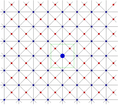
Example 1. The population is arranged on the infinite grid Z⇥Z, where Z denotes the integers. Players are indexed by their location on the grid: Group A players are indexed by the set {(i, j)|i and j both odd}; Group B players are indexed by
{(i, j)|i and j both even}. There are no players located at coordinate (i, j) when ex-actly one of i and j is even. Players k = (i, j) and l = (i0, j0) are neighbours if either (i)ki, i0k=kj, j0k= 1, or (ii) i=i0 and kj, j0k= 2 with i, i0, j, j0 all even, orj =j0 and ki, i0k = 2 with i, i0, j, j0 all even. The network is depicted in Figure 1 below. Group
A players are denoted by red circles, Group B players are denoted by blue circles, and connections between players are denoted by lines. The larger blue circle in the middle of Figure 1 is player (0,0).
Now let us consider contagion thresholds. The goal is to highlight that there can be more than one. By Theorem 2 above, in looking for minimal contagion-inducing sets, we can restrict attention to the monotonic operator ˆ.
Consider first setting X ={(0,0)}[{( 1, 1),( 1,1),(1,1),(1, 1)}. This set is enclosed by the green square in Figure1. In period 1, Group B players ( 2,0),(0,2), (2,0) and (0, 2), will all adopt action 1 provided B 3/8. In period 2, Group B
players ( 2,2),(2,2),(2, 2) and ( 2, 2), will also follow suit if B 3/8. From here,
it is clear that if A = 1/2, then Group A players will adopt and full contagion will
result. Thus, our first contagion threshold is (1/2,3/8).
Now suppose we choose X = {(0,0)}. It is clear that none of the Group A play-ers ( 1, 1),( 1,1),(1,1) or (1, 1) will adopt action 1 given that A is constrained
to be greater than 1/2. However, player (0,0)’s neighbours from Group B, namely ( 2,0),(0,2),(2,0) and (0, 2), will adopt provided B 1/8. It is clear that more
and more Group B players will adopt every period. And given that Group A players are connected only to Group B players, it does not matter what value A takes - full
contagion will result. Thus, our second contagion threshold is (1,1/8).
u u u u u u u u u u u u u u u u u u u u u u u u u u u u u u u u u u u u u u u u u u u u u u u u u u u u u u u u u u u u u u u u u u u u u u u u u u u u u u u u u u u u u u u u u u u u u u u u u u u u u u u u u u u u u u u u ~ @ @ @ @ @ @ @ @ @ @ @ @ @ @ @ @ @ @ @ @ @ @ @ @ @ @ @ @ @ @ @ @ @ @ @ @ @ @ @ @ @ @ @ @ @ @ @ @ @ @ @ @ @ @ @ @ @ @ @ @ @ @ @ @ @ @ @ @ @ @ @ @ @ @ @ @ @ @ @ @ @ @ @ @ @ @ @ @ @ @ @ @ @ @ @ @ @ @ @ @ @ @ @ @ @ @ @ @ @ @ @ @ @ @ @ @ @ @ @ @ @ @ @ @ @ @ @ @ @ @ @ @ @ @ @ @ @ @ @ @ @ @ @ @ @ @ @ @ @ @ @@ @ @ @ @ @ @ @ @ @ @ @ @ @ @ @ @ @ @ @ @ @ @ @ @ @ @ @ @ @ @ @ @ @ @ @ @ @ @ @ @ @ @ @ @ @ @ @ @ @ @ @ @ @ @ @ @ @ @ @ @ @ @ @ @ @ @ @ @ @ @ @ @ @ @ @ @ @ @ @ @ @ @ @ @ @ @ @ @ @ @ @ @ @ @ @ @ @ @ @ @ @ @ @ @ @ @ @ @ @ @ @ @ @ @ @ @ @
Figure 1: Network of Example 1.
4
Robustness to Revision Protocol
In general, predictions in large population models can be sensitive to the revision pro-tocol, i.e., who acts and when. In this section I show that when contagion results, it will do so forarbitrary revision protocols. First I must formally define what I mean by arbitrary revision protocols.
Definition 4. A sequence of action profiles {st}1
t=0 is a generalised best-response
se-quence if it satisfies the following:
(ii) if limt!1st(j) = a2S, then for all T 0, a2 (st|j) for some t T.
It is clear that a generalised best-response sequence includes the best-reply dynamic as a special case. The concept of contagion must be amended slightly for this new definition. This is done as follows.
Definition 5. Action 1 is contagious by generalised best-responses in Language Game
{(N,⇧,⇠),G}, if there exists a finite subset X⇢N, such that every generalised best-response sequence {st}1
t=0 with s(j) = 0 for allj 2N \X, implies limt!1st(j) = 1 for
allj 2N.
An important word in Definition5above is ‘every’. That is, we are free to choose the initial set of adopters as we like (all we must be sure of is that there is some minimal set of agents, X, that must be included), and once we chose this initial set, we are completely free to choose any revision protocol we like. Contagion will still result. We have the following Theorem.
Theorem 3. Fix a Language Game {(N,⇧,⇠),G}. Then, action 1 is contagious by the best-reply dynamic in social network (N,⇧,⇠) if and only if it is contagious by generalised-best-responses in (N,⇧,⇠).
The proof of Theorem 3 is virtually identical to a result in Takahashi and Oyama (2013), who study contagion in the bilingual game, and is therefore omitted.10 It uses the fact that the Language Game is a supermodular game using the (strict) partial order, 0 < 1. As in the proof of Theorem 2, the set of agents required for contagion with respect to arbitrary revision protocols need not coincide with the minimal set that induces contagion under the best-reply dynamic. The point is that if a finite set of agents can induce contagion under the best-reply dynamic, then it is possible to find a (potentially larger, but still finite) set that also induces contagion for any revision protocol satisfying Definition5.
In the next section I study the Language Game on finite networks. The question of contagion, in particular as formulated by Morris, is no longer appropriate as one could
10In the bilingual game, a homogeneous population interact with a symmetric 3⇥3 game of
simply choose the entire population as the initial (finite) set of adopters. However, interesting questions can still be asked. In particular, the issue of equilibrium selection, using the concept of stochastic stability (Foster and Young, 1990; Kandori, Mailath, and Rob, 1993; Young, 1993), can be addressed. I focus primarily on what properties of the network will allow each group to internally coordinate on their preferred action. I use a particular noisy dynamic, where the revision protocol is sequential with only one player responding every period, and the likelihood of choosing the inferior action, “making a mistake”, is payo↵ dependent. (This is the “logit” dynamic first introduced inBlume(1993).) I should note that unlike Theorem 3above, the selected equilibrium is not robust to the revision protocol nor the mistake model (see Neary (2013)); I choose to focus on sequential best-responses and logit mistakes because of an interesting connection that emerges between the failure to coordinate across groups, and cohesive sets being the driving factor for contagion in the infinite model.
5
Finite Networks and Equilibrium Selection
In order to study the Language Game on finite networks, some additional notation is needed. Concerning the network: the size of Group A and B is denoted by NA and
NB respectively, and the size of the whole population byN; for any two nonempty sets
of agentsQ0 and Q00, the set of edges connecting those sets is given by E(Q0, Q00), and
the number of edges connecting those sets by e(Q0, Q00). Concerning strategic aspects:
S denotes the action space and s a typical action profile. Particular interest will focus on the action profile where s(i) = 0 for all i 2 A, and s(j) = 1 for all j 2 B. This profile will be denoted (0,1). Lastly, so that the results for each group can be stated in a symmetric manner, it will be convenient to reverse the meanings of B and 1 B.
That is, for an agent in GroupK 2⇧, coordination on his desired action profile earns him a payo↵ of K.
5.1
Stochastic Stability
As before, time is discrete, begins att = 0, and goes forever. Undiscounted utilities are received every period. At the beginning of a period, one player is randomly drawn (each with equal likelihood) from the population, and this player is a↵orded the op-portunity to revise his current action.11 (From here on I will refer to action profiles as “states” in “state space”S.) When called to act, a player takes a myopic best-response against the current state, correctly forecasting the behaviour of everyone else to remain unchanged.
Any dynamic with these features induces a time-homogeneous nonergodic Markov Process on state space S, with transition matrix that I denote by P. By assuming that an agent may occasionally choose a suboptimal action, an ergodic Markov process, with transition matrix P", that is “close to” the original process P, is generated. (P" is sometimes called a perturbation of P.) Since P" is ergodic, it possesses a unique stationary distribution,µ". As shown byFoster and Young(1990) andYoung(1993),µ" is “close to” one of the (potentially) many stationary distributions ofP,µ? := lim"
#0µ". The following is the main definition.
Definition 6. State s is stochastically stable, or selected, if µ?(s)>0, and uniquely so if µ?(s) = 1.
Intuitively what happens is this. First suppose mistakes never happen. When a player is a↵orded a revision opportunity, he takes a best-response to the current state. Coupling this with the revision protocol generates the transition matrix, P. When mistakes are added, all transitions that could happen underP are still possible, however, there are now additional transitions that could also happen - those that happen when a player accidentally chooses an action that is not a best-response. Thus, allowable transitions under P" include those that could happen under P, and some additional ones. While adding these mistakes means that the system is always in flux, the
now-noisy process spends the bulk of time localised around a subset of the equilibria - the stochastically stable ones.
11This revision protocol is known asasynchronous learning (Binmore and Samuelson,1997;Blume,
2003). However, Al´os-Ferrer and Netzer (2010) show that for all “Best-Response Potential Games” (Voorneveld, 2000), logit mistakes coupled with any any specification of revision opportunities, will select the same equilibrium. Since the Language Game is a potential game (Shapley and Monderer,
1996) - a strict subset of the set of best-response potential games - the result holds true for any revision protocol. (The other most common protocol is independent inertia (Noldeke and Samuelson, 1993;
Computing µ? is the objective. As shown by Bergin and Lipman (1996), µ? is de-pendent on how mistakes are parameterised. I assume the payo↵-dependent, “logit”, mistakes ofBlume (1993) whereby the likelihood of playing a particular action is expo-nentially related to its expected payo↵. As shown in Appendix A, computing µ? with this mistake model is simplified since the Language Game is a potential game (Shapley and Monderer,1996). The potential for the local interactions are as given in (6) and the potential for the game as a whole by that in (7). TheoremA shows that for this noisy dynamic, the state(s) that maximise(s) the potential function is (are) stochastically stable.
5.2
Equilibrium Selection
If the groups are isolated from each other, so thatE(A, B) ={;}, it is clear what action each would like to coordinate on. The results of Young (2001) Chapter 6, and Peski (2010) for the homogeneous agent model, show that in isolation a group will coordinate upon the locally risk-dominant action regardless of the network structure.12 Thus, decentralised play will lead to a desirable outcome when Pareto-efficiency coincides with risk dominance, and an undesirable outcome otherwise. With E(A, B) = {;}, action profile (0,1) would emerge and all would be happy.
Peski’s result can be interpreted negatively: from the perspective of a social engineer, it is not possible to implement a particular outcome by designing a network and simply
letting people play. That is, varying network architecture has no e↵ect on selection in the standard homogeneous environment - risk dominance will ultimately prevail. A similar question can be asked for the Language Game (though it is not clear how risk-dominance ought be defined in a such a heterogeneous setting - see the discussion at the end of Section 4.1 in Neary(2012)). In particular, what properties must a group’s subnetwork satisfy in order for all its members to adopt the preferred action in the long run? It is intuitive that agents in a given group must not only be well-connected internally, but also must not be overly-connected to those in the other group. The following definition, taken from Young (2001), provides a natural measure of intra-group connectedness that captures perfectly the level of connectedness a intra-group must
12Peski’s result is actually stronger than stated as it holds for arbitrary revision protocols and both
satisfy.
Definition 7. Given a real number p 2 (0,1), say that a subset of agents L ✓ N is p-closely-knit if,
8Q✓L, Q6=;, e(Q, L)
e(Q, Q) +e(Q,N) p (2)
Close-knittedness is related to the concept ofcohesiveness fromMorris (2000).13 As we saw in Definition 2, a group is p-cohesive if for each agent in the group, at least a fraction p of his connections are to those in the group (and hence at most a fraction 1 pof his connections are to those outside the group). By considering only singleton subsets, it is clear that a group of agents is p-cohesive whenever it is p-closely-knit, since for any singleton subset Q, the term e(Q, Q) in (2) is equal to zero. However, the reverse implication need not hold due to di↵erences that arise when considering non-singleton subsets.
At first glance, it might seem unnatural that the terme(Q, Q) appears twice in the denominator (since, by definition it is also included in the term e(Q,N)), and hence one might prefer a definition without it. However, the double counting ofe(Q, Q) has a strategic interpretation that I now explain. Note that sinceQ✓ L✓N, we have that e(Q,N) = e(Q, L) +e(Q,N \L). Using this and rearranging expression (2) above, we have that, for a groupL to bep-closely-knit, for all nonempty Q✓L, it must be that
(1 p)e(Q, L) p e(Q, Q) +e(Q,N \L) (3)
Thus, for a group L to be closely knit, for any subset of the group, (1 p) times the number of edges between the subset and the group, must exceed p times the sum of edges between the subset and itself, and the subset and those outside the group. Again, this may seem a little mysterious until one supposes that those in L are defined by a common behaviour that they, and only they adopt. Expression (3) is then ‘counting’ edges in relation to the subset where behaviour is the same. E↵ectively it is considering
13Caveat: When normalising payo↵s in symmetric binary coordination games, the literature often
assumes that the payo↵from thedesirableoutcome is given by 1 pwherepis less than 0.5 (Morris,
2000). The reason for doing this, is that an agent then needs to see a fraction at least as great aspof his neighbours taking the desired action, in order to be willing to adopt it. In this section however, for each groupK, I have used the single parameter, K, to denote the payo↵from the desired equilibrium
what would happen if those in the subset Q collectively deviated from the action that defines those in the set L. In other words, given that the group L was defined by the behaviour of its agents, if those in subset Q now changed theirs, then they should no longer be considered part of L, and hence as outside of L. In a binary action game where actions are strategic complements, after a collective deviation, these agents inQ will now coordinate with those outside of L (and obviously also with those in Q who also deviated). To put it another way, those in Q have now gone from coordinating with those inLto coordinating with those outside of L(of which they are now a part). With dynamics where the behavioural rule is purely deterministic, like those con-sidered in Morris (2000) and in Sections 2 - 4, a collection of agents simultaneously adopting an action that is a painful unilateral deviation, could not occur without some kind of external coordination device. But in the presence of perpetual mistakes there is always that possibility. In fact, it turns out that each GroupK 2⇧ being (1 K
)-closely-knit is precisely the condition required for each group to coordinate upon their preferred action (and hence for there to be a complete failure to coordinate across the groups).
Theorem 4. Action profile (0,1) is stochastically stable under dynamic if and only if each Group K 2⇧ is (1 K)-closely knit.
Proof. The proof is contained in Appendix B.
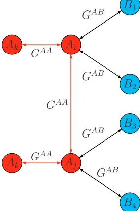
Using Figure 2 below, let’s see why close-knittedness (Definition7) is exactly that which is important for a group to internally coordinate on their preferred action (The-orem 4). Consider the Group A players. For profile (0,1) to be stochastically stable, all subsets of these players must be (1 A)-closely knit. As shown in the proof of
Theorem 4, the important players are those in Group A players who are connected to Group B players; I refer to these players as VA (players A
i and Aj in Figure 2).
First of all, the inequality in (3) must hold for all singleton sets Q = {Ai} ✓ VA. So
each individual player Ai 2VA must have more connections to those in his own group
than (1 A)/ A times the number of connections to those in VB (where VB denotes
those in Group B who are connected to at least one Group A agent). Note that for these singleton sets, this is just a restriction on individual behaviour, since if action 0 is not a best-response for playerAi 2VAto the profile where all other Group Aplayers
equilibrium. (This is precisely Morris’ notion ofp-cohesive, and hence a failure of this criterion for singleton subsets is e↵ectively ruling out profile (0,1) as an equilibrium.) This generates the bound of A <3/4 for (0,1) to be an equilibrium.
However, holding for all singleton subsets of VA is insufficient for the inequality to
hold for all Q ✓ VA as Figure 2 below demonstrates. Agent A
i 2 VA is adjacent to
those in the set VB
1 ={B1, B2} ⇢VB. Agent Ai is also adjacent to agents Aj and Ak
from A. Thus, by taking Q = {Ai}, the relevant inequality holds for any value of A
given that A>1/2>1 A. Similarly, agentAj 2VAis adjacent to two agents from
VB, those in VB
2 = {B3, B4} ⇢ VB. Note that V1B \V2B = ;. Agent Aj is connected
to agents Ai, and Al from Group A. So choosing Q = {Aj}, inequality (3) clearly
holds. However, by choosing Q = {Ai, Aj}, it is the case that e(Q, VB) = 4, whereas
e(Q, A\Q) = 2, and as such inequality (3) will only hold for A 2 [5/8,1) and not for
A2(1/2,5/8).
Figure 2: Failure to coordinate across group.
Figure2hints that the profile (0,1) being stochastically stable might have something to do with robustness to coalitional deviations. But a profitable coalitional deviation need not imply an increase in potential as I now demonstrate. From Figure 2, the threshold at which agentsAi andAj would be made better o↵by collectively deviating
equilibrium. (This is precisely Morris’ notion ofp-cohesive, and hence a failure of this criterion for singleton subsets is effectively ruling out profile (0,1) as an equilibrium.) This generates the bound ofγA <3/4 for (0,1) to be an equilibrium.
However, holding for all singleton subsets of VA is insufficient for the inequality to hold for all Q ⊆ VA as Figure 2 below demonstrates. Agent Ai ∈ VA is adjacent to those in the set VB
1 ={B1, B2} ⊂V
B. Agent Ai is also adjacent to agents Aj and Ak
from A. Thus, by taking Q = {Ai}, the relevant inequality holds for any value of γA given thatγA>1/2>1−γA. Similarly, agentAj ∈VAis adjacent to two agents from VB, those in VB
2 = {B3, B4}⊂ VB. Note that V1B ∩V2B = ∅. Agent Aj is connected to agents Ai, and Al from Group A. So choosing Q = {Aj}, inequality (3) clearly holds. However, by choosing Q = {Ai, Aj}, it is the case that e(Q, VB) = 4, whereas e(Q, A\Q) = 2, and as such inequality (3) will only hold for γA∈ [5/8,1) and not for
γA∈(1/2,5/8).
Ai
B1
B2
Aj
B3
B4 Ak
Al
GAA
GAB
GAB GAA
GAB
GAB GAA
Figure 2: Failure to coordinate across group.
neighbours playing 1, than play 0 and have two neighbours playing 0. That is, the threshold is given by 3(1 A) > 2 , which gives A < 3/5. Since 3/5 < 5/8, there
exist coalitional deviations that increase potential but are not beneficial, or, similarly but opposite, there can be stochastically stable outcomes at which at which profitable coalitional deviations remain unexplored. Refinements of Nash Equilibrium requiring robustness to coalitional deviations have received much attention in the literature but, at least to my knowledge, their relationship to stochastically stable outcomes has so far been unexplored, and an interesting agenda for future research would be to fully classify conditions under which the two can be reconciled.14,15 Clearly they cannot be reconciled in the baseline threshold model as studied in Morris (2000), Ellison (1993), Blume(1993),Young(2011) andPeski (2010), when the common local interaction is a stag hunt since, in this case, stochastic stability selects uniform adoption of the (locally) risk dominant action and not the (locally) Pareto efficient one, so a collective deviation by one an all would be uniformly desirable.
The final result of the paper, Theorem5 below, provides necessary conditions for a symmetric profile to be stochastically stable.
Theorem 5. For a symmetric profile to be stochastically stable, it must be the case that for each group K 2⇧, and each nonempty subsetQ✓K, that
1 K
2 K 1
e(Q, Q)
e(Q,N \Q) (4)
The proof of Theorem 5 is found in Appendix B. I will briefly discuss the intuition here. Condition (4) holds trivially for the group whose preferred symmetric profile is stochastically stable. For the less-content group, what the condition says is that the ratio of the payo↵ at its less-preferred symmetric profile to the payo↵ windfall (the payo↵ from their preferred equilibrium action minus that at their less preferred one)
14Aumann (1959) introduced the notion of astrong equilibrium, where an equilibrium is robust to
unilateral and collective deviations. Bernheim, Peleg, and Whinston(1987) introducedcoalition-proof equilibrium that is similar to strong equilibrium with the extra requirement that the deviation must be to something that is itself self-enforcing. Unfortunately both concepts fail to satisfy existence.
15This statement should not be confused with the works ofPeski(2004) andNewton(2012). In those
must exceed the number of internal edges within the subset Q relative to the number of edges from the subsetQ to those outside it.
6
Conclusion and Extensions
I have looked at how a new behaviour might spread in a setting where part of the pop-ulation would like for it to spread and the remainder of the poppop-ulation would not. The game is the Language Game ofNeary(2012), that is by definition the simplest possible coordination game with heterogeneity that can take place on arbitrary networks, being just a “doubling” of the standard model. My main focus has been on the interplay between network architecture and payo↵s. As regards contagion, the notion of group cohesiveness from Morris (2000) remains the key ingredient, although the definition needs some amending in this heterogeneous setting. As regards equilibrium selection on a finite network, the concept of close-knittedness fromYoung (2001) is what drives results.
APPENDIX
A
Stochastic Stability
Any population dynamic generated by a process as described in the text induces a time homogeneous Markov Process on state space S, with transition matrix P, such that P(s0, s00) 0 denotes the
probability of transitioning froms0 tos00, and for everys2S, P
s0P(s, s0) = 1.
Let 4(S) denote the set of distributions on ⌦. A stationary distribution of P is a row-vector µ2 4(S), such thatµP=µ. The Markov matrixP has at least two stationary distributions, each of which places probability one on a di↵erent symmetric equilibrium. Thus, while repeated applications ofP will lead to an equilibrium, the multiple stationary distributions means that which equilibrium is reached depends on where the play begins. This is known aspath dependence. Foster and Young
(1990) introduced the concept ofstochastically stability that removes this path dependence.
Suppose that there is always a small chance that a player makes a mistake when taking his intended action. This generates a new Markov matrix P", “close to” P. For all "
2 (0,"¯], P" is ergodic and
as such has a unique stationary distribution, denotedµ". Young(1993) shows that lim
"#0µ"=µ? is
unique, and one of the many stationary distributions of the unperturbed processP. The following is the main Definition (a repetition of Definition6).
Definition 8. Statesisstochastically stable, or selected, ifµ?(s)>0, anduniquely so ifµ?(s) = 1.
Computation of µ? can be done uses tree-surgery techniques of Freidlin and Wentzell (1998), originally introduced to game theory in Foster and Young (1990). First, view transitions under P"
as having an associated cost. This cost is captured by the functionc : S⇥S ! [0,1)[{1}, that satisfies the following. For any s0, s00 2 S, (i) c(s0, s0) = 0, and (ii) there exists a path {s1, . . . , sn},
wheres1=s0 andsn=s00, such that c(sm, sm+1)<1form < n.
An s-tree, h, is a function h : S ! S, where a) there is a unique element, sh 2 S, known as
theroot, such that h(sh) = sh, and b) for every s 6=sh, there is a path{s, h(s), . . . , hm(s)}, where
hm(s) = s
h. Withc as the cost function for transitions between states, we can define the cost of an
s-treehas being equal to the sum of the costs of its paths,
c(h) := X
s6=sh
c s, h(s)
Ans-tree is of minimum cost if there is nos-tree of strictly lower cost. For the Language Game where the dynamics have associated cost functionc, denote the set of all roots of minimal costs-trees by
⌦(c) :={s|sis a root ofs-treeh, such that for anys-treeh0, c(h)c(h0)}
The following is the result ofFreidlin and Wentzell(1998) as modified for the Language Game. Note its relation to Definition8above.
Lemma 1. State sis stochastically stable, or selected, ifs2⌦(c), and uniquely soif {s}=⌦(c).
So, fix anN-player game {Si}Ni=1,{Ui}Ni=1 , where, for eachi, Si is playeri’s action set andUi
his real-valued utility function defined onS :=⇥N
j=1Sj.
of others to remain unchanged. If the current population profile is s, and player i is selected, then playerichooses actiona2S according to the probability distribution pi(a|s), where for any >0,
pi(a|s) :=
exp Ui(a;s)
exp Ui(0;s) + exp Ui(1;s)
(5)
Equation (5) above defines the so-called ‘logit response’ function, with mistakes parameterised by the scalar . When = 0, each action is chosen with equal likelihood. As ! 1, the response distribution as defined in (5) approaches that of a best-response. Thus, for any finite , (5) defines a perturbation of the best-response. By combining the perturbed best-response dynamics for each player (assuming that is common across everyone), it is now the case thatµ?:= lim
!1µ .
Since mistakes happen with varying likelihood, the cost of each mistake is not equal and so nor-malisation is useless. This makes direct computation ofµ? a difficult task. But fortunately, given the
particular structure of the Language Game, there is a very workable shortcut. The shortcut exploits the fact that the Language Game is a potential game (Shapley and Monderer, 1996). A game is said to be apotential game if the change in each player’s utility from choosing an action can be derived from a common function, referred to as the game’spotential function. Formally,
Definition 9. An N-person game {Si}Ni=1,{Ui}Ni=1 is a potential game if there exists a function
⇢:S!Rsuch that, for alli2N, alls2S, and all pairss(i)0, s(i)002S
i, we have thatUi(s(i)0;s)
Ui(s(i)00;s) =⇢(s(i)0;s) ⇢(s(i)00;s).
Local interactionsGAA, GAB, andGBB are potential games with respective potential functions16
⇢AA : S
⇥S !R, ⇢AB : S
⇥S ! R, and⇢BB : S
⇥S !R, where each is defined as follows (for
⇢AB, the first argument refers to the GroupAplayer’s action, and the second to the GroupB player’s
action),
⇢AA(0,0) = A ⇢AA(0,1) = 0
⇢AA(1,0) = 0 ⇢AA(1,1) = 1 A
⇢AB(0,0) =
A+ 1 B ⇢AB(0,1) = A
⇢AB(1,0) = 1 B ⇢AB(1,1) = 1 (6)
⇢BB(0,0) = 1 B ⇢BB(0,1) = 0
⇢BB(1,0) = 0 ⇢BB(1,1) = B
Since each local interaction is a potential game, by a straightforward result inNeary (2011), the Language Game is itself a potential game, with potential function,⇢?, where for any action profiles,
⇢?(s) := X
(ij)2EAA
i<j
⇢AA(s(i), s(j)) + X
(ik)2EAB
i2A, k2B
⇢AB(s(i), s(k)) + X
(hk)2EBB
h<k
⇢BB(s(h), s(k)) (7)
The following result is straightforward but key. (It is a direct implication of a Theorem inNeary
(2011), which itself is an extension of a result fromBlume (1993).)
Theorem (Neary(2011)). For every >0,P has the unique stationary distribution,µ , given by
µ (s) = exp ⇢
?(s)
P
s02Sexp ⇢?(s0)
(8)
where ⇢? is the potential function as defined in equation (7). Furthermore, the stochastically stable states are precisely those that maximise the potential function⇢?.
B
Proofs
Proof of Theorem 2.
As stated in the text the ‘only if’ direction is immediate. The ‘if’ direction uses the following Lemma.
Lemma 2. For all nonempty collectionsX, and anyk 1, we have that ˆk(X) =X
[ ˆk 1(X) .
Proof. It is clearly true fork= 1. Suppose it is true for arbitraryk. Now,
ˆk+1(X) = ˆ ˆk(X)
= ˆk(X)[ ˆk(X)
=X[ ˆk 1(X) [ ˆk(X)
=X[ ˆk(X)
where the second equality follows by the definition of ˆ , the third by the inductive hypothesis, and the fourth by dropping the second term in line 3 since if ˆk 1(X)
✓ ˆk(X), then we must have
ˆk 1(X) ✓ ˆk(X) .
So suppose thatX is contagious with respect to ˆ . Since all players were assumed to have a finite number of neighbours, consider the setSv2XNv, which must also finite. ClearlyX ⇢Sv2XNv. Now,
since limk!1ˆk(X) =N, there exists anl 2N, such thatSv2XN ✓ ˆl(X). It is enough to show
that ˆl(X) is contagious with respect to . To get this, fixm > l. By Lemma2 above, for allm 1
and any nonempty setX, we have that
ˆm(X) =X
[ ˆm 1(X)) (9)
But since we chosem > l, we also have that ˆm 1(X)
◆ ˆl(X) X. So equation (9) simplifies to
ˆm(X) = ˆm 1(X))
But since the choice ofmwas arbitrary (the only requirement was thatm > l), it can easily be shown by induction that for allm > l, that
m l ˆl(X) = ˆm(X)
Proof of Theorem 4.
I prove only the result for GroupA, who must be (1 K)/ K -closely knit if and only if (0,·) is to
be stochastically stable. The analogous statements for GroupB is shown in an identical manner.
The ‘if’ direction is easily shown by showing the contrapositive. That is, suppose that (0,·) is not stochastically stable, and let us see that this means GroupAcannot be (1 K)/ K -closely knit.
Lets? denote the stochastically stable equilibrium. Since (0,
·) is not stochastically stable, define the setQ:={i2A|s(i)?= 1}✓Adenote the (nonempty) subset of Group A who take actionb at
action profiles?. Note that, without loss of generality we can assume i) that all players in GroupB
take actionbat the stochastically stable equilibrium, and ii) thatQ✓VAsince, given assumption (i),
these GroupA agents will contribute more towards the potential function by choosing action b than those inA\Q.
Now, consider the contribution towards the potential function when all players inQchoose action b over that when they are all compelled to choose actiona. Since (0,1) is not stochastically stable, we have, using the values from the potential function in (6), that
e(Q, Q)·(1 A) +e(Q, A\Q)·0 +e(A\Q, A\Q)· A+e(Q, VB)·1>
e(Q, Q)· A+e(Q, A\Q)· A+e(A\Q, A\Q)· A+e(Q, VB)· A
Dropping the term that is equal to zero, cancelling the e(A\Q, A\Q)· A term that appears on
both sides, and a moving thee(Q, VB)
· A term to the left hand side, we get that,
e(Q, Q)·(1 A) +e(Q, VB)·(1 A)> e(Q, Q)· A+e(Q, A\Q)· A
Rearranging this, we have thus found aQ⇢Awho are not sufficiently closely-knit.
To show the ‘only if’ direction, start by assuming that⇢?is maximised at (0,1). We will see that this
implies that GroupAmust be sufficiently closely-knit.
Let⇤A ⇢S denote the set of states where all GroupB players are constrained to take actionb.
Consider the discrete time process where players inAupdate their action according to (5). Let P A
denote this irreducible process on state space⇤A with states . As in Theorem A, it can be shown
that the restricted processP A has unique stationary distribution,µ A, where
µ A( ) = exp ⇢
?( )
P
02⇤Aexp ⇢?( 0)
Fix a state = ( 1, . . . , N)2⇤A, and note that
⇢?( ) = X
(i,j)2E(A,A)
⇢AA( (i), (j)) + X
(h,k)2E(A,B)
⇢AB( (h), b) + e(B, B)⇢BB(b, b)
For any two sets X, Y, define X\Y := X\Yc, where Yc denotes the complement of Y. Now,
lettingQ0={i2A: (i) = 1}, it is easy to see that,
⇢?( ) =⇢AA(a, a)·e(A\Q0, A\Q0) +⇢AA(b, b)·e(Q0, Q0) +⇢AB(b, b)·e(Q0, VB) +⇢AB(a, b)·e(A\Q0, VB) +⇢BB(b, b)·e(B, B)
= A·e(A\Q0, A\Q0) + (1 A)·e(Q0, Q0) + 1·e(Q0, VB)
and that
⇢? (0,1) =⇢AA(a, a)
·e(A, A) +⇢AB(a, b)
·e(A, VB) +⇢BB(b, b)
·e(B, B) = A·e(A, A) + A·e(A, VB) + B·e(B, B)
Thus,
⇢? (0,1) ⇢?( ) = Ae(A, A) + Ae(A, VB) Ae(A\Q0, A\Q0)
(1 ↵)e(Q0, Q0) 1e(Q0, VB) ↵e(A\Q0, VB)
= A⇥e(A, A) e(A\Q0, A\Q0) +e(A, VB) e(A\Q0, VB)⇤
⇥
(1 A)·e(Q0, Q0) +e(Q0, VB)⇤
= A⇥e(A, Q0) +e(A, VB) e(A\Q0, VB)⇤
⇥
(1 A)·e(Q0, Q0) +e(Q0, VB)⇤
= A⇥e(Q0, A) +e(Q0, VB)⇤
⇥
(1 A)·e(Q0, Q0) +e(Q0, VB)⇤
= A⇥e(Q0, Q0) +e(Q0, A\Q0) +e(Q0, VB)⇤
⇥
(1 A)·e(Q0, Q0) +e(Q0, VB)⇤
We want conditions onQ0 such that the above is positive. IfQ0=;, then = (0,1) and the above
expression is zero. So without loss of generality suppose restrict attention to nonemptyQ0. Attention can also be restricted to setsQ0 such that Q0\VA
6
= ;, since otherwise e(VB, Q0) = 0 and all the
terms in the last line above are positive meaning the desired inequality follows trivially. Thus it is sufficient that
e(Q0, Q0) +e(A\Q0, Q0) e(Q0, Q0) +e(Q0, VB)
1 A
A
holds for all nonemptyQ0✓AwithQ0\VA6=;.
In fact, we can make the stronger restriction thatQ0 ✓VA, rather thanQ0\VA
6
=;, by noting that, if the inequality in (3) holds forQ✓VA, then it holds for any ˆQ
✓Awhere ˆQ\VA=Q.
To see this, let denote the state in which agents Q ✓ VA take action b. Specifically Q =
i2VA| (i) = 1 . Now consider a state ˆ where ˆ(i) = 1)i2Q, withˆ Q✓Qˆ ⇢Aand ˆQ\VA=Q.
It is sufficient to show that
⇢?( ) ⇢?(ˆ) 0
which must be true since,
⇢?( ) ⇢?(ˆ) =⇥⇢? (0,1) ⇢?(ˆ)⇤ ⇥⇢? (0,1) ⇢?( )⇤
=⇥ A·e( ˆQ, A) (1 A)·e( ˆQ,Q)ˆ ⇤ ⇥ A·e(Q, A) (1 A)·e(Q, Q)⇤
= A·e( ˆQ\Q, A) (1 A)·e( ˆQ,Q) +ˆ q·e(Q, Q)
= A·e( ˆQ\Q, A) (1 A)·⇥e(Q, Q) +e( ˆQ\Q,Qˆ\Q) +·e( ˆQ\Q, Q)⇤
+ (1 A)·e(Q, Q)
= A·e( ˆQ\Q, A) (1 A)·e( ˆQ\Q,Q)ˆ
>0
ˆ
Q✓A. This concludes the proof.
Proof of Theorem 5.
Suppose without loss of generality that profile (0,0) is stochastically stable and consider all nonempty subsetsQ✓B. Clearly it is not profitable for any collection of GroupAagents to deviate from this profile (and clearly doing so would lower the potential), so we must only show that condition (4) holds for allQ✓B where|Q| 2. Furthermore, we need only consider connected subsets Q.
Since Q ✓B, we can view B as two distinct subsets, Q and B\Q. There are thus six types of edges to consider:
1. e(A, A)
2. e(Q, Q)
3. e(Q, B\Q) 4. e(B\Q, B\Q) 5. e(Q, A)
6. e(B\Q, A)
Suppose that those in GroupQchange their action from 0 to 1. Beforehand, we can consider the potential at profile (0,0). Note that after those in Q change their action to 1, the potential along types of edges1,4, and6 will be unchanged. So we need only compare the change in potential along the other types of edges. Appealing to the values in (6), for (0,0) to be stochastically stable, it must be that,
e(Q, Q)·(1 B) +e(Q, B\Q)·(1 B) +e(Q, A)·( A+ 1 B) e(Q, Q)· B+e(Q, A)· A
which implies that
e(Q, Q)·(1 B) +e(Q, B\Q)·(1 B) +e(Q, A)·(1 B) e(Q, Q)· B
References
Adam, E. M., M. A. Dahleh, and A. Ozdaglar (2012): “On Threshold Models
over Finite Networks,” ArXiv e-prints.
Al´os-Ferrer, C., and N. Netzer (2010): “The logit-response dynamics,” Games
and Economic Behavior, 68(2), 413 – 427.
Aumann, R. J. (1959): “Acceptable points in general cooperative N-person games,”
in Contribution to the theory of game IV, Annals of Mathematical Study 40, ed. by R. D. Luce, and A. W. Tucker, pp. 287–324. University Press.
Bandiera, O., and I. Rasul (2006): “Social Networks and Technology Adoption in
Northern Mozambique,” The Economic Journal, 116(514), 869–902.
Banerjee, A., A. G. Chandrasekhar, E. Duflo, and M. O. Jackson (2013):
“The Di↵usion of Microfinance,”Science, 341(6144).
Bergin, J.,andB. L. Lipman(1996): “Evolution with State-Dependent Mutations,”
Econometrica, 64(4), 943–956.
Bernheim, B., B. Peleg, and M. D. Whinston (1987): “Coalition-Proof Nash
Equilibria I. Concepts,” Journal of Economic Theory, 42(1), 1 – 12.
Binmore, K., and L. Samuelson (1997): “Muddling Through: Noisy Equilibrium
Selection,” Journal of Economic Theory, 74(2), 235 – 265.
Blume, L., D. Easley, J. Kleinberg, R. Kleinberg, and E. Tardos (2011):
“Which Networks are Least Susceptible to Cascading Failures?,” in Foundations of Computer Science (FOCS), 2011 IEEE 52nd Annual Symposium on, pp. 393–402.
Blume, L. E. (1993): “The Statistical Mechanics of Strategic Interaction,” Games
and Economic Behavior, 5(3), 387 – 424.
(2003): “How noise matters,” Games and Economic Behavior, 44(2), 251 – 271.
Conley, T. G., and C. R. Udry (2010): “Learning about a New Technology:
Pineapple in Ghana,” American Economic Review, 100(1), 35–69.
Easley, D., and J. Kleinberg(2010): Networks, Crowds, and Markets: Reasoning
About a Highly Connected World. Cambridge University Press.
Ellison, G. (1993): “Learning, Local Interaction, and Coordination,” Econometrica,
(2000): “Basins of Attraction, Long-Run Stochastic Stability, and the Speed of Step-by-Step Evolution,” Review of Economic Studies, 67(1), 17–45.
Foster, D., and P. Young(1990): “Stochastic evolutionary game dynamics,”
The-oretical Population biology, 38, 219–232.
Freidlin, M. I.,and A. D. Wentzell(1998): Random Perturbations of Dynamical
Systems (Grundlehren der mathematischen Wissenschaften). New York: Springer Verlag.
Jackson, M. O., and A. Watts (2002): “On the formation of interaction networks
in social coordination games,” Games and Economic Behavior, 41(2), 265–291.
Kandori, M., G. J. Mailath,and R. Rob(1993): “Learning, Mutation, and Long
Run Equilibria in Games,” Econometrica, 61(1), 29–56.
Kandori, M., and R. Rob (1995): “Evolution of Equilibria in the Long Run: A
General Theory and Applications,” Journal of Economic Theory, 65(2), 383–414.
Manski, C. F. (1993): “Identification of Endogenous Social E↵ects: The Reflection
Problem,” The Review of Economic Studies, 60(3), pp. 531–542.
Morris, S.(2000): “Contagion,” Review of Economic Studies, 67(1), 57–78.
Neary, P. R.(2011): “Multiple-Group Games,” Ph.D. thesis, University of California,
San Diego.
Neary, P. R. (2012): “Competing conventions,” Games and Economic Behavior,
76(1), 301 – 328.
Neary, P. R. (2013): “Supplementing Stochastic Stability,” Discussion paper,
Uni-versity of London, Royal Holloway.
Newton, J.(2012): “Coalitional stochastic stability,”Games and Economic Behavior,
75(2), 842–854.
Noldeke, G., and L. Samuelson (1993): “An Evolutionary Analysis of Backward
and Forward Induction,” Games and Economic Behavior, 5(3), 425–454.
Peski, M.(2004): “Small Group Coordination,” Discussion paper, Northwestern
Uni-versity.
Rogers, E. (2003): Di↵usion of Innovations. Free Press, 5th edn.
Samuelson, L.(1994): “Stochastic Stability in Games with Alternative Best Replies,”
Journal of Economic Theory, 64(1), 35–65.
Samuelson, L.,andJ. Zhang(1992): “Evolutionary stability in asymmetric games,”
Journal of Economic Theory, 57(2), 363–391.
Schelling, T. C.(1969): “Models of Segregation,”The American Economic Review,
59(2), pp. 488–493.
(1971): “Dynamic models of segregation,”Journal of Mathematical Sociology, 1, 143–186.
Shapley, L. S., and D. Monderer (1996): “Potential Games,” Games and
Eco-nomic Behavior, 14, 124–143.
Suri, T. (2011): “Selection and Comparative Advantage in Technology Adoption,”
Econometrica, 79(1), 159–209.
Takahashi, S., and D. Oyama (2013): “Contagion and Uninvadability in Social
Networks with Bilingual Option,” Discussion paper, University of Tokyo.
Voorneveld, M.(2000): “Best-response potential games,”Economics Letters, 66(3),
289 – 295.
Young, H. P. (1993): “The Evolution of Conventions,”Econometrica, 61(1), 57–84.
(2001): Individual Strategy and Social Structure: An Evolutionary Theory of Institutions. Princeton, NJ: Princeton University Press.