ANALYSIS OF IRIS AND PUPIL PARAMETERS FOR STRESS
RECOGNITION
Povilas Treigys
1, Virginijus Marcinkeviius
1, Artras Kaklauskas
21
Vilnius UniversityInstitute of Mathematics and Informatics Akademijos str. 4, LT-08663, Vilnius, Lithuania
e-mail: [email protected]
2
Vilnius Gediminas Technical University Faculty of Civil Engineering Saultekio al. 11, LT-10223, Vilnius Lithuania
Abstract. The aim of this study is to automatically identify the iris and pupil of the eye in the video stream and to parameterize the identified structures in order to make assumptions if the subjected is stressed or not. During tests, subjects were given a number of issues which they had to respond by selecting only one correct answer. Visual material was gathered using a helmet-fitted stationary near-infrared camera that recorded iris and pupil of the eye reactions to stimuli. Subsequently it was made an automatic iris and pupil recognition and approximation by curves in the gathered sequence of images. Each change in the pupil size is described by different time series length. Thus, it is impossible to compare the obtained data using the Euclidean distance measures. For this reason, the metrics based on periodograms were used to compare the data series. The differences calculated between the eye pupil reaction to stimuli and question show-up time was introduced in multidimensional scaling algorithms for dimension reduction. It was noticed that the stimuli to the false answers tend to cluster.
Keywords: real-time iris and pupil parameterization; time series analysis; reaction to stimuli; stress detection.
1. Introduction
In this article, we present the results of investigation for detecting the stress of the investigated person while his/her eye structure reaction to test questions was recorded in the video stream. Then the video stream was processed with a view to get the parametric form of the iris and pupil of the eye. Finally, the parameters obtained were investigated by various data mining methods in order to answer the question: is the investigated person stressed?
Basically, eye-tracking is the process during which a glare spot is registered, or eye movements are registered with respect to the head position. Eye-tracking is commonly used in various scientific explorations such as: diagnostics of eye structures, psychology, cognitive linguistics, and product design [10]. No less important application of eye-tracking can enable to detect the stress of the investigated person that is under some environmental stimuli. Mainly, eye-tracking can be achieved in three ways [5], [2]:
x With eyes are covered by special mirror lenses or magnetic field detectors. This eye-tracking manner allows measuring the movements of the eye very
precisely. However, the use of this approach is limited since it is contact dependent.
x When a reflected light from the eyes is recorded in the video stream. In this case, since the pupil size of the eye is sensitive to the intensity of light, the illumination and video recording of the reflected light are performed in near-infrared (NIR) light range. Further, with the aim to detect eye movements, the techniques of image analysis must be applied within the recorded video frame. This approach is beneficial since it is contactless.
x When the eye-tracking is performed by electrical potential measuring devices applied around the eye area. This approach is beneficial since the movements of the eye may be tracked in the darkness or even when the envelope of the eye is closed. However, just like the first approach it is contact-dependent.
It is obvious that if we want to detect stress to environmental stimuli, the second approach fits best. Thus, the methods of the image analysis must be applied in order to detect the position of the eyes in recorded video frames. Consequently, when the position is known, the search of the main anatomical structures such as iris and pupil becomes meaningful.
The information carried by these structures found and how they change in time can be used for biometric identity or driver advertence level estimation. As stated earlier, the most common way to solve suchlike problems is to use an infrared or near-infrared light source. When the eye is exposed to the NIR light source, it creates bright-dark reflection effect of the eye structures in the recorded video stream [5]. Eye detection task may be solved by applying various methods, such as: artificial neural networks, principal component analysis, eigenvector analysis methods or methods that analyse frame colour intensity distributions [20].
Methods that are based on the image analysis may be classified into three classes: pattern, properties, and sample-based [11]. In the pattern-based method, the generic template describing the form of the eye must be defined first. Then the regions of the image are compared with the generic template and the best match indicates the region of the eye. Similar methods perform very well and accurately detect the eye regions, however, the main drawback of pattern-based methods is that they are computationally intense and cannot be used for eye detection in a live video stream. The property-based methods use image intensity characteristics of the eye region such as contrast differences between iris, pupil, and sclera, and colourfulness of the eye anatomical structures. However, this approach for iris and pupil detection is ineffective in low contrast images. Moreover, in many cases, the size of the iris must be known or it must fall into a known interval. The sample-based methods are able to detect eye structures according to eye photometric description. These methods require a huge amount of data that have eye examples of various people at different lightness, colour, or angle conditions. Then the classifiers such as artificial neural networks or Haar cascade classifiers [17] may be trained in order to detect the eyes in a video frame. Another approach that closely relates the sample-based method group is to use colour or edge information of the eye in the image, however, colour intensities heavily depend on the camera’s white balance pre-set and the edges of objects in the image strongly depend on the contrast of the image as well [21]. Iris and pupil detection will be accomplished by means of sample-based methods.
In this investigation, video was recorded by a NIR camera equipped with a 1/3” Sony CCD sensor that works at a resolution of 420 TV lines. The camera was equipped with two NIR light sources as well.
2. Iris and Pupil Detection
One of the main factors that can determine which algorithms should be used for object recognition in digital images is the size of the image. There are methods that cannot be applied on the image due to insufficient image resolution. In most cases it is the search of compromise between the reliability of the
results and the algorithm performance time. That leads to the fact that a lower video stream resolution allows us to fasten the algorithm performance. However, we should be aware that the resolution of 640x480 pixels may be insufficient for a direct iris and pupil detection. In such cases, if the whole face is visible in video, the area of the eyes is calculated according to the detected face in a video frame and the search for the iris and pupil within the selected region is meaningful. Nevertheless, the first step is to identify the edge between iris and pupil. If the edge is detected, then the edge points may be used for the parameter estimation of the iris and pupil in the least-square terms. To solve the iris and pupil identification problem, the authors provide a great amount of methods. Deniz et al. suggested using the integral-differential function that can describe the inner and outer boundary or the eye iris. The main advantage of the proposed function is that the result achieved is not sensitive to varying lighting conditions. Another approach is presented in [12], where the authors used the iris segmentation binary map, followed by the application of a circular Hough [16] transformation. Interesting methods are presented in [19], [20], where the authors suggest to use an edge detection method that relies on maximization of the gradient function and leads to getting inner and outer iris edges. Finally, detection of the pupil may be accomplished by calculating the integral sum of pixel intensities over the defined region in a frame. The minimal sum should point to the location of the pupil; however, such an approach is subject to the presence of photographic noise and non-uniform illumination. Hence, the methods used for iris and pupil detection require image pre-processing by means of mathematical morphology, kernel convolution, or nonlinear filtering [20] in most cases.
performance. Canny has defined three criteria to derive the equation of an optimal filter for step edge detection: good detection, good localization, and clear response (only one response to the edge) [8]. After smoothing the image and eliminating the noise, the next step is to find the edge strength by taking the gradient of the image. Next, non-maximum suppression has to be applied. There are only four directions when describing the surrounding pixel degrees: 0, 45, 90 and 135. Thus, each pixel has to be grouped in one of these directions to which it is closest. Next we check whether each non-zero pixel (x, y) in the image is greater than its two neighbours perpendicular to the gradient direction. If so, keep the pixel (x, y), or else set it to 0. The final phase of the Canny edge detector is to apply the hysteresis threshold. However, for the hysteresis threshold two threshold levels must be known. Then, by thresholding the result after non-maximum suppression at two different levels ( 1 and 2), we obtain two binary
images. The difficulty is that we cannot apply the static threshold level since there are no images with identical properties. For automated threshold level 1
calculation, we use Otsu’s method [13]. The optimal threshold by Otsu’s method is found through a sequential search for the maximum variance [6] of the image pixels intensity histogram. Further, the threshold level 2 is doubled 1. After the parameters 1
and 2 of the threshold have been calculated, we
convert the image at these two levels into binary ones:
T1, T2. For all the unvisited pixels (x, y) in the image we trace each segment in T2 to its end and set them as contour points. At the segment end in the image T2 we seek its neighbours in the image T2. If there are neighbouring pixels in the image, we denote them as contour points too. Finally, after the edge detection has been completed, we apply the circular Hough transform to localize the pupil. In the case of a circle, this model has three parameters: two parameters indicate the centre of the circle and one parameter the radius. To detect a circle of the radius r, the circles of this radius are plotted in the Hough parameter space centered on each edge pixel found in the image. Thus, the array of peaks is formed for each edge pixel. Peak emerges when the circles in the Hough space intersect with each other. Peaks in the Hough parameter space indicate possible centres of the r radius circles. The problem is that we do not know both: where the pupil lies in the image and how big it is. In our case, we iterate the circular Hough transform each time with the different circle radius r and select the highest peak value in the formed peak array. After the parameters for the circle have been selected, we assume that we approximately found the pupil centre coordinates and the iris radius. After we have approximately calculated a radius of the circle and its centre coordinates, the next step is to choose the points that describe the pupil boundary. This is done by varying the circle radius on polar coordinates. In other words, we iterate the angle and the radius in polar coordinates found by the
iterative Hough transform and check whether the image point (x, y) is set to 1. If so, we add it to the boundary point accumulator, or else move further to check another image point (x, y). After the pupil boundary coordinates have been accumulated, we apply the least squares ellipse fitting algorithm to the parametric form of cone calculation, depending on the data set collected. Since our objective is to parameterize the pupil by an ellipse, further least squares algorithm for fitting the ellipse was used. A full description of the algorithm can be found in [1]. By the Fitzgibbon et. al. scheme, the best parameters of the ellipse correspond to an eigen-vector identified by a minimal positive eigen-value. Finally, the same scheme is applied in the iris detection and parameterization, with the constraint that the iris centre coordinates must fall within the area of the detected pupil.
3. Results
Four students of the Vilnius Gediminas technical university took part in this investigation. During the investigation a camera was recording the eye pupil reaction to stimuli from the test beginning till the end. Various questions were submitted to the students during the test, while they had to choose only one correct answer. The test held by students was graded. When the test was finished, the recorded video material was processed frame-by-frame by the means described in the above section with a view to parameterize the iris and pupil of the eye. The parameter set computed by least squares elliptical fitting algorithm was composed of the minor and major axis of the ellipse, relative centre coordinates, and the rotation angle. However, not all parameters were analysed with the view to detect whether investigative subject is stressed of not. It was assumed that the stress of a student may be evaluated from the area change in the eye pupil. However, in this investigation, the rotation of the eyeball was not known, thus it was impossible to calculate the area of the pupil in each frame precisely. Then an approximate area of the pupil was calculated by:
2,
max
~
b
a
pupil
pupil
S
S
,where the pupil a and are pupil b semi-axes of the approximating ellipsis.
Since
S
~
and the precise area of the circle depends only on the radius, in a further investigation we will use the radiusr
~
only:pupil
apupil
br
max
,
~
.the total number of frames. The time series X has N
tests, so it can be described by
^
x
x
x
i
N
`
X
i i i
i T T T
T11
,
12,
,
1 2,
1
,
,
, where Ti 1 and Ti 2 stand for the i the test question show-up and end-up frame number, respectively. For the sake of simplicity, we assume that^
Ti`
i
x
x
x
X
1,
2,
,
is a time series (vector)and Ti is the number of elements of the series. It is important to note that, in general, Ti Tj as i j. It means that different time is needed to answer different test question.
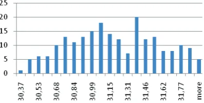
Figure 1. Sample histogram of the eye pupil radius
As Figure 1 shows, an assumption can be made that the radius of the pupil has normal distribution. However, the Kolmogorov-Smirnov test [4] rejects the null hypothesis H0that the random variable has normal distribution with the significance level 0.05. It happens because of the approximation error of the pupil by an ellipse. With a view to filter out outliers that are distant from the series mean value, we applied the rule to the data series. For such data filtering the rule could be applied as well [3]. The standard deviation can be calculated by
¦
Tii i i i
x
E
x
T
1 21
V
,where E(xi) is the arithmetic mean. Then, after the data filtering with the rule, the re-checked null hypothesis
H0 has been satisfied. Figure 2 presents the series histogram.
Figure 2. Histogram of the filtered series
Thus, after filtering and norming the initial data, we get
X
^
X
0,
X
1,
,
X
20`
, where Xi ~N(0,1),X0 is the vector of radii before the first test question show-up time. This vector was omitted from the further investigation. Further, trends of time series have to be explored.
3.1. Moving Average Filtering
Moving average filters are aimed at removing the seasoning effect on the variable xi. According to [3] the variable xi of series Xi can be split into a composition of three:
i i i
i
z
s
u
x
,where zi is a trend component, si is a component of seasoning, and ui is white noise.
Moving average filters are able to decrease or even eliminate the influence of the si and ui components while preserving the coefficients of the polynomials zi. In this case, neither the seasoning nature nor the trend function were known, therefore several moving average filters were applied to eliminate the si and ui
components. The first of the applied moving average filters was a simple mean filter
¿
¾
½
¯
®
]
1
,
1
,
1
,
1
,
1
,
1
,
1
,
1
,
1
,
1
,
1
,
1
,
1
[
25
1
;
25
]
25
[
M
. Thisfilter calculates the average of 25 data points and is able to preserve the first order polynomial coefficients
)
(
a
0a
1t
. Another moving average filter that is able to preserve the fourth order polynomial coefficients was introduced by Spencer [3] and it can be describedas follows: ¿ ¾ ½ ¯ ®
[1,3,5,5,2,6,18,33,47,57,60]
350 1 ; 21 ] 21 [ M .
The results achieved by applying the filter of the data are presented in Figures 3 and 4.
Figure 3.Sample data series for the correct test answer. At the top: initial data series, in the middle: filtered by the moving average filter. At the bottom: Spencer moving average filter has been applied
Figure 4. Sample data series for the incorrect test answer. At the top: initial data series, in the middle: filtered with moving average filter. At the bottom: Spencer moving average filter has been applied
3.2. Comparison of Series
It is important to note that the series are of different length, thus it is impossibleto compare two series using the Euclidean distance. In this case, a technique based on the periodogram metrics will be used [9]. For the stationary process Xi its periodogram can be calculated by the formula:
2
1
1
)
(
ji
i
it T
t t i j
X
x
e
T
P
Z
¦
Z ,here
i
X i
j
j
m
T
j
,
,
1
,
2
S
Z
, and»¼
º
«¬
ª
2
i XT
m
i .
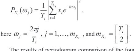
The results of periodogram comparison of the four students during the test are presented in Figure 5.
Considering that for different Xi we have a
different number of elements Ti we use a reduced periodogram comparison approach. The difference is that the frequency is calculated by:
ij i
p
p
m
T
p
,
,
1
,
2
S
Z
,where
min(
,
)
j
i X
X
ij
m
m
m
. Then the distancebetween Xi and Xj can be calculated as follows:
¦
ij i jm
p
p X p X ij j
i
RP
P
P
m
X
X
d
1
2
)]
(
)
(
[
1
)
,
(
Z
Z
.
After calculating the distances between all Xi, a symmetric matrix
D
of distances is obtained. Further, such a matrix can be visualized by multidimensional scaling methods [7]. For the sake of simplicity, we use the principal component analysis method. This method finds new points in the n- dimensional space, such that the corresponding distances from the matrixD
andFigure 5. Test results of the four students applying the principal component analysis method to compare periodogram
Figure 5 presents the stress state of the four students that took the test. Projection points are decoded in the following way: a point represents the correct test answer while the circle represents the incorrect test answer. As it can be seen from the figure, the points tend to group together, i. e., it shows that the periodograms are similar which means that the students are stressed as well. Figure 6 shows the periodogram comparison results when the time series were pre-processed by the Spencer moving average filter. It is obvious that this filtering improves the series projection results. However, to be precise, we need to check thehypothesis
H
0:
f
Xi(
Z
p)
f
Xj(
Z
p)
,where
f
Xi(
Z
p)
is the spectrum function ofX
i.4. Conclusions
In this article, an algorithm is presented for automatic iris and pupil recognition and approximation by curves in the gathered sequence of images. The task was solved by using the Haar classifier for finding the eye region. Further, the detected region was passed to the algorithms for image edge detection and pattern recognition. Finally, parametric estimates of the identified structures were obtained using the least-squares algorithm. The analysed parameter set, composed of ellipses for iris and pupil approximations, described long and short axes. A preliminary data analysis has revealed that an ellipsis that approximates pupil or iris of the eye can be replaced by a circle of radii equal to the major semi-axis of the ellipsis. However, for a better accuracy it is required to assess the spatial eyeball rotation angle.
It is impossible to compare the obtained data using the Euclidean distance measures. For this reason, the metrics based on periodograms were used to compare the data series. The differences calculated between the eye pupil reaction to stimuli and the question show-up time were introduced to multidimensional scaling algorithms to reduce dimensions. We have noticed that stimulitothe false answers tend to cluster, in contrast to stimuli to the correct answers.
Application of different moving average filters to reduce noise has improved the evaluation of similarity (dissimilarity) between the reactions to stimuli. Furthermore, the projections of reactions to stimuli of distinct investigative have yielded different results even when the Spencer moving average filter was introduced. These results suggest that the metrics based on periodograms can be used to spot if the investigated subject is stressed.
We have illustrated that time series of reactions to stimuli have a normal distribution and for the future research, it is expedient to verify the hypothesis on the equality of peridogram spectrum functions.
References
[1] A.Fitzgibbon, M. Pilu, R. B. Fisher. Direct least-squares fitting of ellipses. IEEE Transactions on Pattern Analysis and Machine Intelligence. 1999, vol. 21, no. 5, p. 476-480. ISSN: 0162-8828.
[2] A.Bulling, J.Ward, H. Gellersen, G. Tröster. Eye Movement Analysis for Activity Recognition Using Electrooculography. IEEE Transactionson Patter Analysis and Machine Intelligence (TPAMI). 2011, vol. 33, no. 4, p. 741-753. ISSN: 0162-8828.
[3] C. Gourieroux, A. Monfort. Time series and dynamic models. (G. Gallo, Mont.; G. Gallo, edt.) Cambridge: Cambridge University Press. 1997. ISBN: 0-5214-2308-2.
[4] F. J. Messey. The Kolmogorov-Smirnov Test for Goodness of Fit. Journal of the American Statistical Association. 1951, vol.46 no. 253, p.68-78.ISSN: 0162-1459.
[5] H. D. Crane, C. M. Steele. Generation-Vdual-Purkinje-imageeyetracker. Applied Optics.1985, vol. 24, no. 4, p. 527-537. doi:10.1364/AO.24.000527.
[6] H. Tian, S. K. Lam, T. Srikanthan. Implementing Otsu's Thresholding Process Using Area-Time Efficient Logarithmic Approximation Unit. IEEE International Symposium on Circuits and Systems (ISCAS). 2003, vol. 4p. 21-24.ISSN: 0271-4310.
[7] I. Borg, J. P. Groenen. Modern Multidimensional Scaling: Theory and Applications (SecondEdition). NewYork: Springer. 2005. ISBN: 0-3879-4845-7.
[8] J. A. Canny. Acomputational approach to edge detection. IEEE Trans. Pattern Anal. Mach. Intell. 1986, vol.8, p. 679-698. ISSN: 0162-8828.
[9] J. Caiado, N. Crato, D. Peña. Comparison of time series with unequal length. Munich Personal RePEc Archive. 2007.
[10] J. G. Daugman. High confidence visual recognition of persons by a test of statistical independence. IEEE Trans. Pattern Analysis and Machine Intelligence.
1993, vol. 15 no.11, p. 1148-1161. ISSN: 0162-8828.
[11] J. Zhai, A. Barreto. Stress Detection in Computer Users Throughout Non-Invasive Monitoring of Physiological Signals. Biomed Sci Instrum. 2006 vol. 42, p. 495-500. ISSN: 0067-8856.
[12] L. Liam, A. Chekima, L. Fan, J. Dargham. Iris recognition using self-organizing neural network.
IEEE, Student Conf. On Research and Developing Systems. 2002, p. 169–172. ISBN: 0-7803-7565-3.
[13] N. Otsu. A threshold selection method from gray-level histograms. IEEE Trans. Syst. Man Cybernet. SMC91(1). 1979, p. 62-66.ISSN: 0196-2892.
[14] O. Deniz, M. Castrillon, J. Lorenzo, L. Anton, M. Hernandez, G. Bueno. Computer vision based eye wear selector. Journal of Zhejiang University – Science C. 2010, vol. 11, no. 2, p. 79-91. ISSN: 1869-196X.
[15] Open Source Computer Vision Library reference
manual. Intel. 2010. http://opencv.itseez.com/modules/refman.html.
[16] P. V. C. Hough. A method and means for recognizing complex patterns, U. S. Patent 3069654, 1965.
on Computer Vision and Pattern Recognition. 2001, vol. 1, p. 511-518. ISSN: 1063-6919.
[18] P. Viola, M. Jones. Robust real-time object detection. Inernational Journal of. Computer Vision. 2004, vol. 57, no. 2, p. 137-154.ISSN: 0920-5691.
[19] R. D. Labati, V. Piuri, F. Scotti. Neural-based iterative approach for iris detection in iris recognition systems. IEEE international conference on Computational intelligence for security and defense applications. 2009. ISBN: 978-1-4244-3763-4.
[20] R. P. Wildes. Iris Recognition: An Emerging Biometric Technology. Proceeding of the IEEE. 1997, vol. 85, no. 9 p. 1348-1363. ISSN: 0018-9219.
[21] T. Elbert, W. Lutzenberger, B. Rockstroh, N. Birbaumer. Removal of ocular artifacts from the EEG. A biophysical approach to the EOG.
Electroencephalogr Clin Neurophysiol. 1985, vol. 60, p. 455-463. ISSN: 0013-4694.