R E S E A R C H
Open Access
Population allocation at the housing unit
level: estimates around underground
natural gas storage wells in PA, OH, NY,
WV, MI, and CA
Drew R. Michanowicz
1*, Samuel R. Williams
1,2, Jonathan J. Buonocore
1, Sebastian T. Rowland
3,
Katherine E. Konschnik
4, Shaun A. Goho
5and Aaron S. Bernstein
1,6Abstract
Background:Spatially accurate population data are critical for determining health impacts from many known risk factors. However, the utility of the increasing spatial resolution of disease mapping and environmental exposures is limited by the lack of receptor population data at similar sub-census block spatial scales.
Methods:Here we apply an innovative method (Population Allocation by Occupied Domicile Estimation–ABODE) to disaggregate U.S. Census populations by allocating an average person per household to geospatially-identified residential housing units (RHU). We considered two possible sources of RHU location data: address point locations and building footprint centroids. We compared the performance of ABODE with the common proportional population allocation (PPA) method for estimating the nighttime residential populations within 200 m radii and setback areas (100–300 ft) around active underground natural gas storage (UGS) wells (n= 9834) in six U.S. states. Results:Address location data generally outperformed building footprint data in predicting total counts of census residential housing units, with correlations ranging from 0.67 to 0.81 at the census block level. Using residentially-sited addresses only, ABODE estimated upwards of 20,000 physical households with between 48,126 and 53,250 people living within 200 m of active UGS wells–likely encompassing the size of a proposed UGS Wellhead Safety Zone. Across the 9834 active wells assessed, ABODE estimated between 5074 and 10,198 more people living in these areas compare to PPA, and the difference was significant at the individual well level (p= < 0.0001). By either population estimation method, OH exhibits a substantial degree of hyperlocal land use conflict between
populations and UGS wells–more so than other states assessed. In some rare cases, population estimates differed by more than 100 people for the small 200 m2well-areas. ABODE’s explicit accounting of physical households confirmed over 50% of PPA predictions as false positives indicated by non-zero predictions in areas absent physical RHUs.
(Continued on next page)
© The Author(s). 2019Open AccessThis article is distributed under the terms of the Creative Commons Attribution 4.0 International License (http://creativecommons.org/licenses/by/4.0/), which permits unrestricted use, distribution, and reproduction in any medium, provided you give appropriate credit to the original author(s) and the source, provide a link to the Creative Commons license, and indicate if changes were made. The Creative Commons Public Domain Dedication waiver (http://creativecommons.org/publicdomain/zero/1.0/) applies to the data made available in this article, unless otherwise stated. * Correspondence:michanow@hsph.harvard.edu
1Center for Climate, Health and the Global Environment, Harvard T.H. Chan
School of Public Health, 401 Park Drive, Landmark Center 4th floor west suite 415E, Boston, MA 02215, USA
(Continued from previous page)
Conclusions:Compared to PPA–in allocating identical population data at sub-census block spatial scales–ABODE provides a more precise population at risk (PAR) estimate with higher confidence estimates of populations at greatest risk. 65% of UGS wells occupy residential urban and suburban areas indicating the unique land use conflicts presented by UGS systems that likely continue to experience population encroachment. Overall, ABODE confirms tens of thousands of homes and residents are likely located within the proposed UGS Wellhead Safety Zone–and in some cases within state’s oil and gas well surface setback distances–of active UGS wells.
Keywords:Population at risk, Oil and gas, Underground natural gas storage, Safety, Environmental health, U.S. Census, Setbacks
Background
Estimates of the spatial distribution of human popula-tions supports planning and decision-making across a range of domains, including public health, transporta-tion, sustainable development, and climate change resili-ence [1–3]. Public health research often relies on estimates of the population at risk (PAR), or the number of individuals who may experience known risk factors of disease [4–8], as well as natural and manmade hazards [2, 9–11]. Such estimates support epidemiology, expos-ure assessment, and first-order risk analysis research that assesses the potential impact of an exposure. However, coarse spatial resolution of population data, relative to exposure and hazard location data, has limited advances in estimating PAR for a variety of hazards.
In the United States, population data are publicly available at aggregated aerial units (e.g., census blocks and tracts), and typically represent nighttime residential population since census surveys capture where respon-dents reside, rather than time spent working and travel-ing. Unfortunately, when this population data is applied to health research, these data lead to the classic aerial unit problem (AUP), referring to the statistical biasing observed in a spatial analysis when the geographic con-text or scale is modified [12]. Studies that rely on census data or similar data to estimate PAR are constrained by the AUP and therefore are required to make assump-tions about the spatial structure of populaassump-tions– typic-ally the assumption that populations are homogeneously distributed within aerial units (i.e., proportional weight-ing). Such assumptions are often not explicitly stated, are rarely valid, introduce uncertainly, and are increas-ingly important for spatially discrete phenomena and risk regimes such sea level rise, hazardous containment areas, audible warning systems, and explosion blast radii, among others.
Dasymetric mapping techniques can improve propor-tional population allocation (PPA) methods by allocating census population counts to likely habitable land uses [13–15], but still estimates populations at an area-scale, and therefore relies upon the assumption of uniform population density within those habitable areas.
Population allocation at a discrete location such as a residential housing unit (defined by the U.S. Census as a house, apartment, group of rooms, or a single room oc-cupied or intended for occupancy as a separate living quarters) can attenuate the AUP by avoiding to work at area-scales and thus avoids the assumption of uniform population density across space. Remote sensing tech-nologies can provide more accurate representations of population spatial heterogeneity [2, 16–19], and have been utilized to estimate populations at the individual building/household scale [20–23]. However, building/ household-level predictions have been limited to small study areas, and widescale population allocation to discrete locations such as physical buildings been ultim-ately limited by the availability and quality of residential housing location data.
Here, we first test the efficacy of three geospatial data sources to proxy for residential housing unit (RHU) lo-cations: building footprint data, and two publicly-available address datasets (OpenAddresses.io and the U.S. Department of Transportation’s National Address Database). We then present the population allocation by occupied domicile estimation (ABODE) method that dis-aggregates census block data to discrete RHUs and com-pare it to the common proportional population allocation (PPA) method by enumerating populations living within 200 m of active underground natural gas storage wells (UGS) in six U.S. States. Additionally, we apply ABODE to estimate the number of households and populations within very small areas around UGS wells–state oil and gas surface setback area regulations where applicable. While some studies have provided the-oretical evidence that such setbacks–the minimum dis-tance which an occupied structure must be set back from a well –may not be protective of health or safety [24,25], few have relied on geospatial physical dwelling data to describe extant land use conflicts that could re-sult from population encroachment and the general lack of reverse setback rules.
obsolescence issues identified at UGS facilities (e.g., single-point-of-failure well designs) have placed new scrutiny on the hazards they may pose to nearby popula-tions [26–28]. Second, the Interagency Task Force on Natural Gas Storage Safety, which was formed after the 2015 Aliso Canyon leak, recommended that “ stake-holders should collect and analyze data on the proximity of UGS facilities to population centers to help better quantify some of the risk factors”[27]. Our development of spatially-precise PAR estimates directly responds to this request. Third, though many UGS facilities were ori-ginally sited at city limits decades prior, population en-croachment from urban and suburban sprawl has likely created an understudied area of potential land use con-flicts and PAR to low probability/high impact loss of containment events. Fourth, although numerous studies have attempted to quantify populations potentially at in-creased risk of adverse health effects due to their prox-imity to active oil and gas operations [11,29], UGS wells have largely been excluded from these analyses due to poor well location data availability. Finally, small area population estimates are also informative for assessing consistency with a Wellhead Safety Zone that the Oak Ridge National Laboratory has recently proposed for UGS wells based upon individual well diameter and op-erating pressure [30].
Methods
Study areas
First, we selected UGS wells in states based upon: 1) prevalence of UGS operations (e.g., total facilities, wells, and working gas); 2) total populations of census blocks in which UGS wells are located; 3) address and building data availability and quality; 4) a history of UGS inci-dents; 5) facility- and well ages; and; 6) variability in le-gislative building setback distances. Based on our criteria, we chose UGS wells in Pennsylvania (PA), Ohio (OH), New York (NY), West Virginia (WV), Michigan (MI), and California (CA). For each of these states, we compared PAR estimates from ABODE and PPA under two search distances. The first search distance was 200 m, which corresponds to the U.S. Federal Pipeline Haz-ardous Materials Safety Administration (PHMSA) high consequence area designations intended to mitigate harms from pipeline explosions to adjacent communities [49 U.S.C. § 192.5(a) [1]]. PAR estimates for 200 m radii also likely represent a lower bound of a proposed Well-head Safety Zone for active UGS wells- based on the area that would on average exceed a 5000 Btu/hr-ft2 ra-diant heat flux during the first 30 s of an explosion [30]. The second search distance varied by state, and repre-sented each state’s individual surface setback distance, which ranged from 100 to 300 ft. NY (100 ft), OH (100 ft), PA (200 ft), MI (300 ft), and WV (200 ft) (CA does
not have building setback rules) (See Additional file 1: Table S4 for additional detail). Surface setbacks are one regulation-based strategy that is intended to protect the health and safety of residents by setting an exclusion area around a well that shall not contain an occupied dwell-ing. While these setback rules are typically intended for new producing wells, applicability to certain well types including UGS wells varies by state.
UGS well data
We used previously published data on UGS facilities and wells from Michanowicz [26]. Well counts included all active wells connected to active UGS facilities from the April 2016 Energy Information Administration-191 M
Monthly Underground Gas Storage Report [31]. The six states selected contain 179 UGS facilities and 9834 active wells, representing 47% of facilities and 61% of active UGS wells nationwide. The UGS facilities in these states handle on average 2.1 Bcf, totaling 44% of national stored gas capacity.
Spatial accuracy of UGS well location data by visual inspection
To assess the spatial accuracy of the publicly available well data, we performed a visual verification of wellhead locations for a simple random lottery selection of 5% of wells in each state. Reported well locations were com-pared to visual appearance in aerial images across sea-sons from two sources: the 2.5 - 15 m TerraColor imagery (Earthstar Geographics LLC, imagery) from the Landsat 8 satellite (2013–2017), and the 0.5–1.0 m im-agery from the National Agriculture Imim-agery Program (NAIP) administered every 3 years by the U.S. Depart-ment of Agriculture Farm Services Agency. For each well, we either calculated an offset distance between the reported coordinates and the observed location or re-ported the well as “unidentified.” We took measures to prevent misclassifying well location accuracy during the visual inspection. If a well could not be identified within a search area of 1000 ft2from the administrative coordi-nates or could not be distinguished among multiple wells in the area, then the location was reported as“ un-identified.”The percentage of wells visually verified, and their median offset distances are presented in Table1.
Population allocation by occupied domicile estimation (ABODE)
address and building points that resided in commercial, industrial, or institutional parcels (See Additional file 1: Table S2 for complete listing of land use types). The remaining candidate locations were then assigned as ‘residential housing units’ (RHUs) to represent discrete locations of nighttime residential populations. Because ABODE relies on identification of physical dwellings, both populations and counts of occupied dwellings in an area can be reported.
Address and building location data
Residential housing units are defined by the U.S. Census as a house, apartment, group of rooms, or a single room occupied or intended for occupancy as a separate living quarters. Candidate data consisted of two types – ad-dress coordinate points, and geospatial building foot-prints/centroids. Address location coordinate points were available (as of October 23, 2017) from the US De-partment of Transportation’s National Address Database (NAD) (NY, OH) and OpenAddressess.io (PA, WV, MI) originally sourced from state geographic information systems departments, the U.S. Postal Service, and county property parcel datasets [32, 33]. Geospatial building footprints and centroids were available via academic use waiver for various parts of the country from Building-FootprintUSA (BFUSA, Albany, NY). Address location data were not available for California and certain coun-ties of PA and MI (e.g., twelve PA councoun-ties missing ad-dress data), and therefore only building footprint data or manual entry could be applied in these well areas. Not-ably, address data from the NAD and OpenAddresses.io were assumed to account for multi-residential unit buildings (i.e., multi-family apartment complexes) through duplicate address coordinate points, whereas building location data only provided the location of a building, without indication of whether it was a single residence or a multi-unit building.
Residential housing units
In order to censor only potential RHU’s within residen-tial areas, we applied a dasymetric filter. Based on the 2010 land use parcel model from Theobald [34] at 30 ×
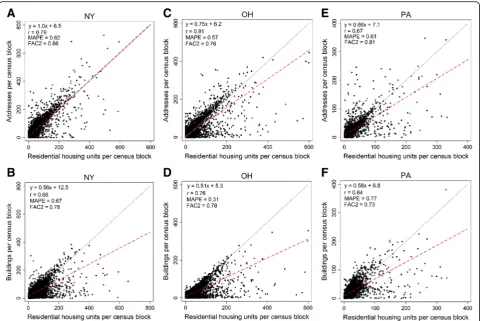
30 m resolution, candidate address and buildings that intersected with built-up (BU) commercial, industrial and institutional use grid cells were excluded from the final RHU list (see Additional file 1: Table S2). Add-itional file1: Table S2 also shows the counts of land use parcels that correspond with all addresses located within 200 m of an active UGS well. RHU counts from each method were summed at the census block level and compared to RHU counts from the 2010 U.S. Census. This comparison was performed for all census blocks within two randomly selected counties of each NY, OH, and PA that contained complete coverage for both ad-dress and building data. In predicting total counts of housing units from the census at the census block level, we presented one-to-one plots, correlation coefficients (Spearman), mean absolute percentage errors (MAPE – with zero predictions removed) and FAC2 which de-scribes the fraction of data that satisfy
0:5≤ Candidate RHUs
Census housing units≤2:0 ð1Þ
The dataset that best predicted U.S. Census RHU counts at the census block level across the two counties of each NY, OH, and PA was selected for the subsequent ABODE estimations for all six states.
Spatial accuracy of residential housing unit locations at state setback distances
To assess the accuracy of the building and address loca-tion data, and resolve reliable RHU estimates within state setback distances, a visual inspection was per-formed for only the well-areas that initially overlapped with a candidate RHU corresponding to applicable state surface setback rules. UGS wells that did not initially intersect with candidate RHU data were not visually inspected. Therefore, RHUs were visually verified around UGS wells in NY (100 ft), OH (100 ft), PA (200 ft), MI (300 ft), and WV (200 ft). Though CA does not have building setback rules, all CA RHUs were manually im-puted due to limited address/building data. Visual in-spection utilized similar aerial imagery products
Table 1Visual verification of well locations
State Active UGS
facilities // wells
Wells visually
verifieda Visually unidentifiedwellsa Median (SD) visualoffset distance (ft.)
CA 12 // 346 17 5 10.9 (7.4)
MI 39 // 2394 119 4 10.9 (8.2)
NY 26 // 972 48 4 52.3 (174.8)
OH 21 // 3318 166 26 55.5 (117.3)
PA 46 // 1332 67 11 62.7 (126.5)
WV 25 // 1472 73 30 82.8 (131.3)
a
described above and entailed removing RHUs that did not appear to represent an inhabitable structure, and no RHUs were added during this inspection process. Visually-verified RHUs were then carried through to subsequent ABODE 200 m RHU counts and population estimates. Generally, address location data correspond to one of four distinct physical location types: 1) physical buildings (e.g., building footprint centroids), 2) land par-cels containing a building, 3) land parpar-cels without build-ing(s), and 4) point at nearest street segment (e.g., mail box location). Generally, address points from criteria“3” were the only candidate RHUs removed. See Additional file 1: Figure S5 for examples of address location types described herein, and Additional file1: Table S4 for re-sults of visual verification. Address and residential hous-ing unit data assumptions and anticipated biases are presented in Additional file1: Table S1.
Population at risk
For each well, we first defined an area (j),representing a radial buffer area around each well drawn using the 200 m search radii. For each given area j, we first identified the number of residential housing units within each cen-sus blocki, partially or completely contained within the areaj,as denoted byRHUijin eq. (2).
Xn
i¼1RHUij ð2Þ
The U.S. Census provides the average ‘person per household’ (i.e., “average household size”- T064_001 from the U.S. Census of Population and Housing Sum-mary File) at census block i denoted by pphi which equates to the total population of census blocki (exclud-ing populations in group quarters) divided by the total number of housing units within that same block. Total population of an area jcan then be calculated by sum-ming the product of the count of residential housing units that intersect with areajmultiplied by the average person per household for census block i at as show in eq. (3).
Popj¼Xn
i¼1RHUijpphi ð3Þ
It is important to note that eq. (3) fails to account for populations residing in group quarters (e.g., prisons, uni-versity dorms). Certain care should be taken at the out-set to account for the presence of group quarters populations injareas of interest that intersect with cen-sus group quarters populations. Within each cencen-sus block, the number of RHUs that contributed to the PAR was capped at the number of housing units reported by the census to help avoid possible inflation from includ-ing non-residential addresses or post 2010 housinclud-ing unit growth–referred to“capped RHU/ABODE” henceforth.
Uncapped population estimates were also reported for comparison (“ABODE”) and may reflect new population-and residential housing unit growth between 2010 population-and 2018. The publishing dates of address data typically at county-level ranged between 2009 to 2018 (See Add-itional file1: Table S5).
ABODE estimates were then compared to a common proportional population allocation (PPA) area weighting approach that allocates census population density (i.e., persons per square mile) to an area of interest. To calcu-late the number of people in area j using PPA, first all 200 m well-area polygons were dissolved to prevent doubling counting then intersected with census block polygons. The overlapping census block segments were then clipped to the well-areas and new geometric areas were calculated. These calculated areas were then multi-plied by the population density of the residing census block to resolve a population estimate that could be summed across all clipped census block segments. To compare PPA and ABODE estimates, we presented well-level prediction differences (ABODE minus PPA) across states with a focus on disagreement scenarios that high-lights PPA false positives (i.e., PPA predicts positive pop-ulations, yet no RHUs are present) (Fig. 2). We also reported one-to-one plots (Additional file 1: Figure S3), tests of equal variances, FAC2, and fractional bias (FB) explained by:
FB¼1 n
Pn
1ABODE−PPA
Pn
1
ABODEþPPA
2
0 B @
1 C
A ð4Þ
where ABODE and PPA represent populations predic-tions for individual well-areas for nwells per state. Sta-tistics were performed using STATA v. 14.2 (College Station, TX), and R v. 3.2.2. (R Core Team, 2019).
Results
The accuracy of publicly available UGS well location data varied by state. MI and CA well locations were more accurate than northeastern states as indicated by proportions of unidentified wells (beyond a 1000 ft. search radius) and shorter offset distances in MI and CA from visual inspection via aerial imagery (Table1).
to residentially-sited buildings (NY: r= .79 vs. 66; OH:
r= .81 vs. 0.76; and, PA: r= 0.67 vs. 0.64, respectively) . There also are differences in deviations from the one-to-one lines between address and building data as indicated by the slope of the liner fit lines, MAPE, and FAC2 values. While OH buildings did produce a smaller MAPE compared to addresses (0.31 vs. 0.57 -Fig. 1, panels c and d), apportioning populations to buildings would likely result in systematic PAR under-estimations in part due its inability to capture multi-dwelling units (e.g., apartment complexes), which are more likely captured by address data. Moreover, the buildings data in OH represents only 84% of the total residential housing units, compared to the 114% of addresses vs. census housing units. Thus, for both data types, candidate RHU counts may disagree with census counts because of temporal misalignment; a portion of RHU location data is likely more recent and may account for changes subsequent to the 2010 census such as new housing development. Address data representativeness ranged at the county level from 2009 to 2018 (Additional file 1: Table S5).
Of addresses from OpenAddresses.io and the National Address Database (NAD) that intersected the 200 m2 well-areas, nearly 65% fell within built-up residential areas (exurban > urban > suburban) as per the Theobald [34] land use classification model (See Additional file1: Table S2). Given the relatively high resolution of this land use model (30 × 30 m), this observation supports the assumption that these address data are sufficiently spatially accurate and sufficiently proxy for census-provided RHUs across various population morphologies (i.e., urban to rural). This observation also highlights the unique land use conflicts presented by UGS systems that were originally cited near city limits many decades prior and have since experienced population encroachment. Considering these results, we elected to use address lo-cation data over building data to proxy for RHUs for census population disaggregation across all six states for consistency, and RHUs henceforth refer to residentially-sited addresses. This decision is considered precaution-ary when considering the preference to overestimate PAR rather than underestimate. In acknowledging sub-optimal address quality, RHUs located within setback
well-areas (likely a higher risk class) were visually inspected via aerial imagery, and results are reported in Additional file1: Table S3.
Uncapped RHU counts were greater than census block housing unit counts by 10, 8, and 19% for the two se-lected counties in PA, OH, and NY (Fig.1), and the dif-ferences were significant (PA: p= <.0001; OH:
p= <.0001; NY: p= <.0001). Under the assumption that overestimates could be due to inclusion of non-residential domiciles (i.e., empty parcels), rather than new RHU development following the 2010 census, we capped RHUs so that they do not exceed counts of housing units within an individual census block. Capped ABODE estimates no longer overestimated census-reported RHU counts for the selected counties, instead differences were−13,−12%, and−4%, respectively. Not-ably, this adjustment only impacts total RHU and popu-lation enumerations, not intra-block RHU spatial heterogeneity. The capped and uncapped ABODE esti-mates in Table2therefore reflect the assumptions of po-tential address misclassification (capped) and popo-tential new population/housing unit growth (uncapped).
By either allocation method–ABODE or PPA– thou-sands of people and homes are likely within the pro-posed UGS Wellhead Safety Zone, and in some cases within state oil and gas well surface setback distances (See Table 4 and Additional file 1: Figure S2). By the PPA method, an estimated 43,052 people live within 200 m of the 9834 active UGS wells across the six states assessed (Table 2), while ABODE predicted between 48, 126 and 53,250 (capped and uncapped) people within the same areas. Population differences between PPA and capped ABODE were significant at the well level (z = 12.5, n= 9834, p= < 0.0001, Wilcoxon signed-rank test). Notably, 6108 of the 200 m well-areas contained zero RHU’s; however, PPA only correctly predicted a zero population for 1082 of these areas, whereas ABODE cor-rectly predicted zero for all 6108. In other words, PPA produced a false-positive non-zero population estimate for at least 5026 well-areas–over 50% of the total well-areas assessed. This difference can be understood
through the underlying processes of the two methods – ABODE assumes residence in discrete spaces (i.e., phys-ical structures), whereas PPA assumes some amount of population across continuous space. For ABODE, areas that do not contain an RHU do not contain people, whereas PPA does not check for RHUs when counting population. Thus, compared to PPA–in allocating iden-tical census data to sub census block areas –ABODE’s discretionary allocation provides more precise PAR esti-mates by reducing PAR misclassification that occurs when PPA counts people in areas that do not contain RHUs.
In general, ABODE captured higher populations within 200 m of wells in OH, WV, and PA, with lower bound increases of 6% (1591), 54% (1081), and 48% (2425), respectively, compared to PPA estimates. Con-versely, ABODE captured lower populations in CA (− 26% or 321). ABODE had similar estimates to PPA for NY and MI where PPA estimates fell within the bounds of capped and uncapped ABODE (see Table 2). Differ-ences between methods were statistically significant for CA, MI, NY, WV, and PA, but not for OH (Table2, and Additional file1: Figure S3). A portion of the population difference observed in CA is likely driven by data quality via manual housing unit identification that likely under-represented multi-dwelling units akin to using building data alone to represent RHUs. Population differences be-tween methods were not mediated by the number of census blocks included or mean block area, and census block area was a poor predictor of census block popula-tions (R2= .02, RMSE = 67).
A comparison of PPA vs. ABODE by state demon-strates the differences at the individual well level both across and within states (Fig.2 & Additional file 1: Fig-ure S3). In some cases, population estimates differed by more than 100 people between the two methods for in-dividual 200 m-radius well-areas. Not surprisingly, the PPA method tends to overpredict populations when no physical housing units are present (Fig.2, panel a - red markers). This was particularly prominent in MI where PPA predicted greater-than-zero estimates around 269
Table 2Population estimates and RHUs within 200 m of active UGS wells
State Wells (% total) with at least one RHU
Uncapped RHUs PAR (PPA) PAR (ABODE) PAR (Uncapped ABODE) Well-level Wilcoxon Signed-Rank (Z) Ho: PPA = ABODE
CA 41 (12%) 400 1216 895 939 3.11*
MI 668 (28%) 2027 4740 4283 5158 6.64***
NY 362 (38%) 996 2495 2393 2691 3.81**
OH 1680 (51%) 12,014 27,593 29,184 31,273 1.11 (p= 0.2)
PA 577 (43%) 3709 4996 7421 9336 −5.99***
WV 488 (33%) 1791 2012 3093 3853 0.79***
Total 3816 (41%) 20,937 43,052 48,126 53,250 12.5***
*
wells that did not contain any housing units within 200 m. Table 3 lists the top ten individual wells across the six states ranked by capped ABODE. Five of the top ten wells identified by ABODE did not make the top ten ac-cording to PPA–for three of these wells, PPA underes-timated PAR by more than 100 people. Only 41 of CA’s 346 UGS wells contained an RHU within 200 m – the lowest percentage of the six states assessed. However, two wells in the Playa Del Rey field in CA ranked first and third respectively in the number of RHUs, and the esti-mated populations within 200 m indicate that UGS well-population relationships are not necessarily generalizable at the state or facility level. Nonetheless, UGS wells in OH, PA, MI, NY, and WV exhibited a much higher degree of land use conflicts in both magnitude and proximity compared to CA UGS wells.
Of the 9384 UGS wells assessed across five states (there are no setback rules for CA wells), 444 wells asso-ciated with 69 storage facilities contained at least one RHU within its state’s regulated setback distance (see Table4and Additional file1: Figure S2). This equated to
a total of 905 visually verified RHUs (304 were manually removed) corresponding to an estimated 2171 people living within their home state’s setback. MI exhibited the most setback conflicts between wells and RHUs, but also promulgates the largest setback distance of the states in-cluded (300 ft). Similarly, over half of PA and WV facil-ities contained at least one well with a setback conflict.
In line with 200 m results, PPA underestimated popu-lations living within setback distances of wells in PA and WV; however, unlike PAR estimates at 200 m, PPA tended to overestimate ABODE at the smaller buffer areas for MI and OH. This suggests that PPA and other aerial weighting population allocation techniques are likely less reliable with decreasing search radii as the likelihood of capturing RHUs decreases with decreasing search radii. In other words, the distinction between areas of homogeneous density and discrete points of nighttime residential population is sharper at smaller spatial scales. Fig. 3 illustrates the principle that spatial heterogeneity of RHU’s can impact PAR estimates. For example, the dark blue 200 m well-area indicates that
A
B
PPA overestimated the ABODE population by 65 (PPA estimated 65; ABODE estimated zero). Less than 400 m from this well location and in the same census block, the well-area in red was estimated to contain 81 people according to PPA–69 fewer people than ABODE’s esti-mate of 151 people.
Figure3 also demonstrates at sub-census block scales how PPA systematically breaks down compared to ABODE when the assumption of evenly distributed pop-ulations is violated –which it often is. Here we observe a patterned relationship between RHUs (grey points) and roadways (yellow) –that in many areas also double as census block boundaries (black lines). ABODE can ac-count for this common pattern of homes (and residents) along roadways/census boundaries by first requiring RHUs in the search area prior to allocating population, whereas PPA treats all areas as if RHUs are evenly dis-tributed within the block. Therefore, under this type of RHU/roadway pattern, PPA for small search areas that overlap with roadway/block boundaries will systematic-ally underestimate the true population (i.e., true nega-tive) and produce many false positives elsewhere. It is also important to note that census block sizes and shapes vary significantly across space and are not deter-mined or controlled for by total population counts like census tracts, as indicated by the poor association
between census block area and total population (R2= 0.02; see Additional file1: Figure S4).
Discussion
The goals of this study were: 1) to develop a housing unit level population allocation method using appropri-ate address location- and building data spanning numer-ous states; 2) to apply these methods to estimate nighttime residential population at risk to UGS wells across six U.S. States; 3) to compare results to common aerial weighting estimates (e.g., PPA) at the sub-census block level to determine potential imprecision in similar PPA-PAR studies, and; 4) to utilize the curated RHU lo-cations to assess the explicit spatial relationships be-tween physical households and UGS wells in relation to the proposed UGS Wellhead Safety Zone and regulatory setbacks, where applicable.
Many studies have quantified populations at potentially higher risk of adverse health and safety effects due to their proximity to active oil and gas operations [35–40]. Most recently, Czolowski, Santoro [11] observed similar dis-crepancies across PAR proximity studies stemming pri-marily from inconsistent inclusion criteria for wells and ancillary infrastructure. However their national PAR esti-mates would likely not vary much vs. ABODE due to the relatively large search radii (one mile) that effectively
Table 3Top ten wells ranked by ABODE population at risk within 200 m
Storage field State RHUs PAR (Capped ABODE) PAR (PPA) PAR difference PPA PAR rank
1. Playa Del Rey CA 150 341 375 −34 1
2. Zane Storage OH 142 318 259 58 3
3. Playa Del Rey CA 107 283 234 48 6
4. Medina OH 88 257 87 170 109
5. Oakford PA 146 255 127 128 43
6. Murrysville PA 98 244 201 43 10
7. Stark-Summit OH 95 236 176 59 16
8. Stark-Summit OH 81 222 66 155 156
9. Stark-Summit OH 95 221 162 59 20
10. Stark-Summit OH 77 221 203 18 9
Table 4Population estimates and RHUs within state setbacks of active UGS wells
State Applicable state
setback distance (ft.)a Facilities // wellswith setback conflict Visually verified RHUswithin Setback PAR (PPA) PAR (ABODE)
CA NA NA NA NA NA
MI 300 16 // 153 344 1277 532
NY 100 5 // 10 10 64 27
OHa 100 9 // 65 83 724 401
PA 200 25 // 124 296 550 792
WV 200 14 // 92 172 246 419
Total – 69 // 444 905 2861 2171
a
reduces the total surface areas around wells that come in contact with non-whole census block areas–the intersti-tial areas where ABODE treats RHUs differently than PPA. McKenzie, Allshouse [29] applied a similar housing unit population allocation to assess population dynamics in Colorado using third-party real estate addresses geo-coded with Google Maps. Our methods differed by using residentially-censored and publicly-available address loca-tion data with a persons-per-household estimate from the residing census block, as opposed to an aggregate multi-county average. Our study also further explored the implications of using discrete household geographic infor-mation to assess PAR using ABODE, particularly in com-parison to PPA techniques and in relation to very small search areas such as state setbacks spanning 100-300 ft2.
A major limitation of all similar distance-based studies is the availability and quality of oil and gas well data,
which can vary across facility, state, and over time [41]. While we did perform a limited sensitivity on well loca-tional accuracy, a true visual verification would require an onsite inspection. Nonetheless, the range of locational accuracies observed herein underscores the importance of accuracy of both RHU proxy data and the hazard of interest when attempting to estimate PAR.
Because population estimates rely on census data, the primary sources of error are attributable to correctly identifying RHUs – both in terms of misclassification and temporal misalignment. It is important to note these errors can independently impact the efficacy of ABODE which could be conflated when comparing to other methods such as PPA. While we attempted to characterize potential for misclassification of RHUs, it is much more difficult to apportion errors to potential temporal misalignment between population data (2010),
and address data that ranged between 2009 and 2018 (See Additional file 1: Table S5). Residentially-sited ad-dresses from OpenAdad-dresses.io and the partial National Address Database, while better than building data alone, only moderately predicted counts of census housing units, and misclassifications of occupied structures were observed in all states. Because estimates relying on building footprints alone tended to underpredict census housing units–but better captured physical domicile lo-cations over address location–a better proxy for RHUs could be obtained by combining additional ancillary datasets such as parcel data or hybrid address/building data. The ongoing development of the U.S. Department of Transportation’s National Address Database stands to provide an authoritative source of accurate residence ad-dress location data nationwide that could support hous-ing unit population mapphous-ing at larger scales, though much progress is still required [33]. Similarly, advances in remotely sensed object recognition and resolution re-finement [42] have led to the first publicly available data-base of building footprint vector data for the entire U. S that could provide physical locations and verification to link to aforementioned address data [43].
Since residential structures do not move over time, whereas census aggregation units can, population esti-mates anchored to RHUs can attenuate the modifiable areal unit problem. However, some error remains in assuming an average person-per-household size. The number of residents in each household cannot be per-fectly measured without labor intensive surveys; how-ever household sizes could be further refined by using additional information about the residential housing units. A few studies have allocated populations based on building footprint area [22], and building volume estimated from aerial imagery data [20, 23], though these likely perform optimally for larger buildings in more urbanized areas. Estimates at the housing unit level also does not require census survey coverage if remote sensing building data are made available globally, and reasonable estimates of persons per household can be made. It is also important to note that population disaggregation methods that utilize census data are estimating the nighttime residential population- based on where people sleep. This ig-nores mobility of people, and the dynamic nature of populations in space and time, which also can intro-duce exposure and risk misclassification in epidemio-logical studies, and in other applications [44–46].
The major strength of ABODE is that it does not rely on the assumption of uniform spatial homogeneity of populations within an aerial unit. The formulation of ABODE better represents the real world – nighttime residence occurs in discrete locations (homes) rather than continuously across space. Violations of PPA’s
assumption of spatial homogeneity were clearest in well-areas where zero visible RHU structures exist, yet PPA estimated a positive population (greater than zero) for over 50% of the total well-areas assessed. These esti-mates therefore can be confirmed as false positives (see Fig.2). Based on our results across multiple sub-census block search areas, we expect PPA and similar aerial weighting techniques to lose precision and increase the likelihood of false positives with decreasing search radii. In tandem, PAR estimates backed by identification of RHUs provides an improved population density metric that carries a co-benefit of internal validation through the mutual inclusion of people and their physical dwell-ings. Such improved precision has relevance for estimat-ing PAR to hazards with relatively short distance-based thresholds such as explosions, noise, air pollution, odors, sea level rise, radiation, and flooding.
Data presented herein provides new information re-garding how close some homes and residents are to ac-tive UGS wells that are predominately located in suburban areas. The portion of RHUs identified within regulatory setback distances may result from several rea-sons. A significant portion of UGS wells likely predate any setback regulations for conventional wells (setback rules do not generally exist for other types of wells) due to their age (i.e., grandfathering). Other explanations in-clude: 1) misclassification or spatial imprecision of UGS well and/or RHU, 2) a homeowner’s and/or regulatory agency’s consent to waive setback requirements for the drilling of new wells; and/or, 3) setback rules in the states assessed pertain only to placement of new wells in relation to existing buildings, not to the placement of homes in relation to existing wells (i.e., encroachment).
Conclusion
populations and UGS wells – more so than the other states assessed; and, 6) likely tens of thousands of homes and residents are located within the proposed UGS Wellhead Safety Zone –and in some cases within state oil and gas well surface setback distances – of active UGS wells.
Additional file
Additional file 1:SI Figure 1.Methodological workflow and destination of results.SI Table 1.Methodological assumptions, anticipated biases, tests, data adjustments, and implications.SI Table 2.
Number of individual land use parcels intersected by address points located within 200m of an active UGS well across the six states observed. Bold highlighted rows indicated land use types that contain addresses that were censored from inclusion as a residential housing unit.SI Figure 2.Frequency histograms of housing units within 200 m (657 ft) of active UGS well(s) by distance from well. Red lines indicate each state’s applicable regulatory surface setback distance for conventional oil and gas wells. The number displayed represents the number of visually verified housing units within the setback distance. The number displayed in the top right corner signifies total intersects including duplicates.SI Figure 3.PPA vs. ABODE population estimates of areas within 200m of active UGS wells. Dashed lines represent linear fits. Note each state plot contains unique scales.SI Table 3.UGS well and building counts within surface setbacks with visual verification results.SI Table 4.Legislative oil and gas setback restrictions for buildings.SI Figure 4.Total populations at the census block level vs. census block area for all six states assessed.
SI Figure 5.Neighborhood level view of housing unit/address point and well data quality issues.SI Table 5.Address data original sources and publish date. OA = OpenAddresses.io, NAD = National Address Database. (DOCX 85961 kb)
Abbreviations
ABODE:Allocation by occupied domicile estimate; AUP: Aerial unit problem; BU: Built-up; CA: California; MI: Michigan; NAD: National Address Database; NAIP: National Agriculture Imagery Program; NY: New York; OH: Ohio; PA: Pennsylvania; PAR: Population at risk; PPA: Proportional population allocation; RHU: Residential housing unit; RMSE: Root mean square error; SD: Standard deviation; UGS: Underground natural gas storage; WV: West Virginia
Acknowledgements
Not applicable
Authors’contributions
DM and AB designed the study. SW, DM, JB, SR conducted data analyses and visual inspections. KK and SG performed analyses related to legislative setbacks. DM, SW drafted the manuscript and all authors contributed to its contents. All authors read and approved the final manuscript.
Funding
The Heinz Endowments Grant E5489; The Environmental Defense Fund Project Code: 0136–101000-10615.
Availability of data and materials
RHU data are available from corresponding author on reasonable request.
Ethics approval and consent to participate
Not applicable
Consent for publication
Not applicable
Competing interests
The authors declare they have no competing interests.
Author details
1Center for Climate, Health and the Global Environment, Harvard T.H. Chan
School of Public Health, 401 Park Drive, Landmark Center 4th floor west suite 415E, Boston, MA 02215, USA.2Department of Environmental Health, Boston University, Boston, MA 02215, USA.3Department of Environmental Health
Sciences, Columbia University, New York City, NY 10027, USA.4Nicholas
Institute for Environmental Solutions, Duke University, Durham, NC 27708, USA.5Emmett Environmental Law & Policy Clinic, Harvard Law School, Cambridge, MA 02138, USA.6Division of General Medicine, Boston Children’s
Hospital, Boston, MA 02115, USA.
Received: 14 January 2019 Accepted: 13 June 2019
References
1. Saporito S, Chavers JM, Nixon LC, McQuiddy MR. From here to there: methods of allocating data between census geography and socially meaningful areas. Soc Sci Res. 2007;36(3):897–920.
2. Balk D, Yetman G. The global distribution of population: evaluating the gains in resolution refinement. New York: Center for International Earth Science Information Network (CIESIN), Columbia University; 2004. 3. Hay S, Noor A, Nelson A, Tatem A. The accuracy of human population maps
for public health application. Tropical Med Int Health. 2005;10(10):1073–86. 4. Tatem AJ, Campiz N, Gething PW, Snow RW, Linard C. The effects of spatial
population dataset choice on estimates of population at risk of disease. Popul Health Metrics. 2011;9(1):4.
5. Linard C, Tatem AJ. Large-scale spatial population databases in infectious disease research. Int J Health Geogr. 2012;11(1):7.
6. Tatem AJ. Mapping the denominator: spatial demography in the measurement of progress. Int Health. 2014;6(3):153–5.
7. Richardson DB, Volkow ND, Kwan M-P, Kaplan RM, Goodchild MF, Croyle RT. Spatial turn in health research. Science. 2013;339(6126):1390–2.
8. Tatem AJ, Adamo S, Bharti N, Burgert CR, Castro M, Dorelien A, et al. Mapping populations at risk: improving spatial demographic data for infectious disease modeling and metric derivation. Popul Health Metrics. 2012;10(1):8.
9. Hauer ME, Evans JM, Mishra DR. Millions projected to be at risk from sea-level rise in the continental United States. Nat Clim Chang. 2016;6(7):691. 10. Nadim F, Kjekstad O, Peduzzi P, Herold C, Jaedicke C. Global landslide and
avalanche hotspots. Landslides. 2006;3(2):159–73.
11. Czolowski ED, Santoro RL, Srebotnjak T, Shonkoff SB. Toward consistent methodology to quantify populations in proximity to oil and gas development: a National Spatial Analysis and review. Environ Health Perspect. 2017;86004:1.
12. Dorling D. Map design for census mapping. Cartogr J. 1993;30(2):167–83. 13. Mennis J. Dasymetric mapping for estimating population in small areas.
Geogr Compass. 2009;3(2):727–45.
14. Eicher CL, Brewer CA. Dasymetric mapping and areal interpolation: implementation and evaluation. Cartogr Geogr Inf Sci. 2001;28(2):125–38. 15. Bhaduri B, Bright E, Coleman P, Urban ML. LandScan USA: a high-resolution
geospatial and temporal modeling approach for population distribution and dynamics. GeoJournal. 2007;69(1–2):103–17.
16. Stevens FR, Gaughan AE, Linard C, Tatem AJ. Disaggregating census data for population mapping using random forests with remotely-sensed and ancillary data. PLoS One. 2015;10(2):e0107042.
17. Patel NN, Stevens FR, Huang Z, Gaughan AE, Elyazar I, Tatem AJ. Improving large area population mapping using geotweet densities. Trans GIS. 2017;21(2):317–31. 18. Wardrop N, Jochem W, Bird T, Chamberlain H, Clarke D, Kerr D, et al. Spatially
disaggregated population estimates in the absence of national population and housing census data. Proc Natl Acad Sci. 2018;115(14):3529–37.
19. Deville P, Linard C, Martin S, Gilbert M, Stevens FR, Gaughan AE, et al. Dynamic population mapping using mobile phone data. Proc Natl Acad Sci. 2014;111(45):15888–93.
20. Tomás L, Fonseca L, Almeida C, Leonardi F, Pereira M. Urban population estimation based on residential buildings volume using IKONOS-2 images and Lidar data. Int J Remote Sens. 2016;37(sup1):1–28.
21. Xie Z. A framework for interpolating the population surface at the residential-housing-unit level. GISci Remote Sensing. 2006;43(3):233–51. 22. Mathews AJ, Ellis EA. An evaluation of tornado siren coverage in Stillwater,
23. Zhao Y, Ovando-Montejo GA, Frazier AE, Mathews AJ, Flynn KC, Ellis EA. Estimating work and home population using lidar-derived building volumes. Int J Remote Sens. 2017;38(4):1180–96.
24. Banan Z, Gernand JM. Evaluation of gas well setback policy in the Marcellus shale region of Pennsylvania in relation to emissions of fine particulate matter. J Air Waste Manage Assoc. 2018; just-accepted.
25. Haley M, McCawley M, Epstein AC, Arrington B, Bjerke EF. Adequacy of current state setbacks for directional high-volume hydraulic fracturing in the Marcellus, Barnett, and Niobrara shale plays. Environ Health Perspect. 2016; 124(9):1323.
26. Michanowicz DR, Buonocore JJ, Rowland ST, Konschnik KE, Goho SA, Bernstein AS. A national assessment of underground natural gas storage: identifying wells with designs likely vulnerable to a single-point-of-failure. Environ Res Lett. 2017;12(6):064004.
27. Interagency Task Force on Natural Gas Storage Safety. Ensuring safe and reliable underground natural gas storage. NETL-TRS-15-2016. US Department of Energy Office of Fossil Energy Energy Do; 2016. 28. 49 C.F.R § 191 & 192.
29. McKenzie LM, Allshouse WB, Burke T, Blair BD, Adgate JL. Population size, growth, and environmental justice near oil and gas wells in Colorado. Environ Sci Technol. 2016;50(21):11471–80.
30. Sulfredge CD, Rose SD. Development of Wellhead Safety Zone Criteria for Underground Gas Storage Facilities. Oak Ridge: Oak Ridge National Lab.(ORNL); 2018.
31. U.S. Energy Information Administration. 191M - monthly natural gas storage report. 2016.
32. OpenAddresses.io. OpenAddresses. 2018.https://github.com/ openaddresses/openaddresses. Accessed 17 May 2019.
33. U.S. Department of Transportation. National Address Database 2018 [Available from:https://www.transportation.gov/nad. Accessed 17 May 2019.
34. Theobald DM. Development and applications of a comprehensive land use classification and map for the US. PLoS One. 2014;9(4):e94628.
35. Adgate JL, Goldstein BD, McKenzie LM. Potential public health hazards, exposures and health effects from unconventional natural gas development. Environ Sci Technol. 2014;48(15):8307–20.
36. Hays J, McCawley M, Shonkoff SB. Public health implications of environmental noise associated with unconventional oil and gas development. Sci Total Environ. 2017;580:448–56.
37. Shonkoff SB, Hays J, Finkel ML. Environmental public health dimensions of shale and tight gas development. Environ Health Perspect. 2014;122(8):787. 38. Vengosh A, Jackson RB, Warner N, Darrah TH, Kondash A. A critical review of
the risks to water resources from unconventional shale gas development and hydraulic fracturing in the United States. Environ Sci Technol. 2014; 48(15):8334–48.
39. Werner AK, Vink S, Watt K, Jagals P. Environmental health impacts of unconventional natural gas development: a review of the current strength of evidence. Sci Total Environ. 2015;505:1127–41.
40. McKenzie LM, Blair B, Hughes J, Allshouse WB, Blake NJ, Helmig D, et al. Ambient nonmethane hydrocarbon levels along Colorado’s northern front range: acute and chronic health risks. Environ Sci Technol. 2018;52(8):4514–25. 41. Glosser D, Rose K, Bauer JR. Spatio-temporal analysis to constrain uncertainty in
wellbore datasets: an adaptable analytical approach in support of science-based decision making. J Sust Energy Eng. 2016;3(4):299–317.
42. Lin G, Milan A, Shen C, Reid ID, editors. RefineNet: multi-path refinement networks for high-resolution semantic segmentation. Cvpr; 2017. 43. Microsoft Inc. U. S. Building Footprints. 2018.https://github.com/Microsoft/
USBuildingFootprints;.
44. Park YM, Kwan M-P. Individual exposure estimates may be erroneous when spatiotemporal variability of air pollution and human mobility are ignored. Health Place. 2017;43:85–94.
45. Kwan M-P. The uncertain geographic context problem. Ann Assoc Am Geogr. 2012;102(5):958–68.
46. Kwan M-P. The neighborhood effect averaging problem (NEAP): an elusive confounder of the neighborhood effect. Int J Environ Res Public Health. 2018; 15(9):1841.
Publisher’s Note