A novel approach to determine two optimal cut-points of a continuous predictor with a U-shaped relationship to hazard ratio in survival data: simulation and application

(1)

T E C H N I C A L A D V A N C E

Open Access

A novel approach to determine two

optimal cut-points of a continuous

predictor with a U-shaped relationship to

hazard ratio in survival data: simulation and

application

Yimin Chen

1

, Jialing Huang

1

, Xianying He

2

, Yongxiang Gao

1

, Gehendra Mahara

1

, Zhuochen Lin

1

and

Jinxin Zhang

1*

Abstract

Background:In clinical and epidemiological researches, continuous predictors are often discretized into categorical variables for classification of patients. When the relationship between a continuous predictor and log relative hazards is U-shaped in survival data, there is a lack of a satisfying solution to find optimal cut-points to discretize the continuous predictor. In this study, we propose a novel approach named optimal equal-HR method to discretize a continuous variable that has a U-shaped relationship with log relative hazards in survival data.

Methods:The main idea of the optimal equal-HR method is to find two optimal cut-points that have equal log relative hazard values and result in Cox models with minimumAICvalue. An R package‘CutpointsOEHR’has been developed for easy implementation of the optimal equal-HR method. A Monte Carlo simulation study was carried out to investigate the performance of the optimal equal-HR method. In the simulation process, different censoring proportions, baseline hazard functions and asymmetry levels of U-shaped relationships were chosen. To compare the optimal equal-HR method with other common approaches, the predictive performance of Cox models with variables discretized by different cut-points was assessed.

Results:Simulation results showed that in asymmetric U-shape scenarios the optimal equal-HR method had better performance than the median split method, the upper and lower quantiles method, and the minimump-value method regarding discrimination ability and overall performance of Cox models. The optimal equal-HR method was applied to a real dataset of small cell lung cancer. The real data example demonstrated that the optimal equal-HR method could provide clinical meaningful cut-points and had good predictive performance in Cox models.

Conclusions:In general, the optimal equal-HR method is recommended to discretize a continuous predictor with right-censored outcomes if the predictor has an asymmetric U-shaped relationship with log relative hazards based on Cox regression models.

Keywords:Optimal cut-points, Discretization, Categorize, U shape, Cox regression model, Survival analysis

© The Author(s). 2019Open AccessThis article is distributed under the terms of the Creative Commons Attribution 4.0 International License (http://creativecommons.org/licenses/by/4.0/), which permits unrestricted use, distribution, and reproduction in any medium, provided you give appropriate credit to the original author(s) and the source, provide a link to the Creative Commons license, and indicate if changes were made. The Creative Commons Public Domain Dedication waiver (http://creativecommons.org/publicdomain/zero/1.0/) applies to the data made available in this article, unless otherwise stated. * Correspondence:[email protected]

1_{Department of Medical Statistics and Epidemiology, School of Public Health,}

Sun Yat-sen University, Guangzhou 510080, China

(2)

Background

In survival analysis, Cox regression models [1], which are the most popular model in this field, are frequently used to investigate the effects of explanatory variables on right-cen-sored survival outcomes. The explanatory variables may be continuous, such as age or weight, or they may be discrete variables, such as gender or treatment factors. When con-tinuous explanatory variables have nonlinear effects on out-comes, it is of interest to investigate U-shaped relationships [2–5] between continuous explanatory variables and health-related outcomes in many researches. Although the U-shaped effects of continuous variables can be modeled in Cox models with flexible smoothing techniques [6–8], such as penalized splines and restricted cubic splines, many clin-ical and epidemiologclin-ical researchers would rather discretize continuous explanatory variables [9,10] to reflect high-risk and low-risk values of the independent variables and com-pare the risks of developing survival outcomes (i.e. deaths or relapses) between different groups of patients. Moreover, optimal cut-points could help identify thresholds of import-ant predictors, which could be used to provide classification schemes of the patients and assist in making clinical treat-ment decisions. In practice, it is sensible to use standard clinical reference values as cut-points to discretize continu-ous predictors. But when it comes to lack of standard refer-ence ranges for newly discovered risk factors or the reference ranges can’t be applied to the population with dif-ferent characteristics, how to find the scientific and reason-able cut-points to categorize continuous independent variables has been an important issue to be addressed [11– 13].

There are two widely adopted approaches to discretize continuous independent variables in survival analysis. One is the data-oriented cut-points approach [14, 15], which uses the median value, quartiles or other percentile values based on the distribution of continuous variables as cut-points. Owing to its simplicity and easiness of imple-mentation, median value and upper and lower quantiles (noted as Q1Q3) have been widely used in many studies as cut-points. However, this approach provides arbitrary cut-points regardless of the relationships with survival outcomes and might lead to wrong estimates of the true effects. Another approach named maximum statistic ap-proach or minimump-value approach was first developed by Miller and Siegmund [16] to dichotomize continuous predictors with binary outcomes. The minimum p-value approach selects a cut-point with maximumχ2statistic as the optimal cut-point when the outcomes are binary. When it is extended to survival outcomes, the optimal cut-point is the one that results in a minimump-value of log-rank tests [17]. In the simulation studies of the minimum p-value approach, it is usually assumed that there is a single theoretical threshold of continuous variables, which means relationships between independent variables and survival

outcomes are stepwise functional relations. In practice, in-dependent variables and survival outcomes generally have smooth relationships instead of biologically implausible stepwise functional relationships. In addition, U-shaped re-lationships between continuous variables and outcomes are commonly seen in the clinical and epidemiological studies [2–5] but little considered in the study of the discretization methods. In the case of body mass index (BMI), a too low and a high BMI value both cause harmful effects on overall health [3,18]. When a prognostic variable has a U-shaped relationship with outcomes, the effect of the prognostic variable may be underestimated using high and low-risk groups divided by a single cut-point.

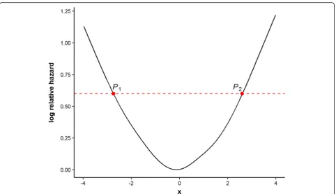
To overcome the shortcomings of the common discretization methods in survival data and meet the needs of finding optimal cut-points for a continuous predictor that has a U-shaped relationship with survival outcomes, we propose a new approach named optimal equal-HR method to estimate two optimal cut-points that have approximately equal log hazard values based on Cox regression models. The main idea of the optimal equal-HR method is derived from the clinical need of classifying patients into high-risk and low-risk groups according to a categorized prognostic variable. In clinical practice, the classification of high-risk or low-risk patients is based on their risks of developing unfavored survival outcomes, such as deaths or relapses. And the larger log relative hazards correspond to the higher risks of developing the observed survival outcomes. Despite the reference ranges, common methods for classification in practical epidemiology studies, such as the Q1Q3 method, are not accurate to define such low-risk or high-risk groups when there exists a U-shaped relationship. It is because the individuals with the same risks (the same log relative hazards) could be divided into opposite risk groups by the Q1Q3 method. During the pro-cedures of finding optimal cut-points, it is important to consider the effects of log relative hazards. Hence, we use log relative hazards to find two optimal cut-points (P1,P2) of the prognostic variableX (as shown in Fig. 1). The pa-tients withXsmaller thanP1or larger thanP2are classified into two high-risk groups (or two low-risk groups in an in-verse U-shaped relationship) respectively. By doing this, the two high-risk groups are defined according to the same threshold of log relative hazards, which makes the classifi-cation more reasonable in clinical explanations. Our method can provide more accurate optimal cut-points and avoid the individuals with the same risks (the same log rela-tive hazards) being divided into opposite risk groups. An R package named‘CutpointsOEHR’has been originally devel-oped to help investigators easily implement the optimal equal-HR method.

(3)

equal-HR method is compared with other commonly used discretization methods regarding discrimination power and overall performance via a simulation study. We present the simulation settings in Section‘The Simulation Study’. The results of the simulation study and the appli-cation of the optimal equal-HR method on a real dataset of small cell lung cancer are presented in Section‘Results’. Finally, there are discussion and conclusions.

Methods

The optimal equal-HR method is based on Cox propor-tional hazards regression models [1] which have the following structure:

h tð Þ ¼h0ð Þt expðβ0XÞ ð1Þ

where h(t) denotes the hazard function,h0(t) denotes the

baseline hazard function,tis the observed survival times,

X is a vector of covariates, andβis a vector of estimated regression coefficients. The relative hazardλcan be calcu-lated as the above equation divided byh0(t) in both side:

λ¼ h tð Þ

h0ð Þt ¼ exp β

0_X

ð Þ ð2Þ

The optimal equal-HR method uses log(λ) values to search for optimal cut-points. Hazard ratios (HR) could

be easily calculated from the relative hazardsλwhen inves-tigators choose a reference value of an independent vari-able and control other varivari-ables at average levels. And the relationship between HR and a continuous variable is iden-tical to that betweenλand the continuous variable. There-fore, the method of finding the optimal cut-points with approximate equal log(λ) values is named as optimal equal-HR method. The procedure of the optimal equal-HR method contains two main steps described as follows.

Graphical diagnostic plot

The optimal equal-HR method proposed in this study aims to solve the problem of discretizing a continuous variable that has a U-shaped relationship with log(λ) in the Cox model. Therefore, the first step of adopting the optimal equal-HR method is to determine the relationship between a continuous covariate and log(λ) and plot the curve. Previous researches have already proposed several methods for estimating nonlinear relationships, including the multiple β method [19], martingale residual based method [20], spline methods [21], etc. The performance of the multipleβmethod for Cox models is unstable and largely depends on the number of selected groups because a Cox model is a semi-parametric model and its likelihood is based on the order of events rather than their distribu-tions. The martingale residual based method, which uses

(4)

martingale residuals from Cox models to test the log-linearity, cannot plot the relationship between a con-tinuous covariate and log(λ). Due to the limitations of the above two methods, this study used Cox regression models with penalizedB-splines (P-splines) [7,22], which balances goodness of fit and variance, to curve the relationship and determine whether the non-linear term is statistically sig-nificant. The smoothing parameter of theP-splines of de-gree 3 with 22 evenly spaced knots is automatically chosen by minimizing AIC, which is achieved through the R-function‘pspline’in the‘suevival’package under the uni-variate situation. If there are two or above couni-variates with nonlinear effects, the R-function ‘dfmacox’ in the

‘smoothHR’package [23] could be used to obtain the opti-mal smoothing parameter. Then the estimated log(λ) values are plotted against the continuous variable to give an insight into the biological nature of the continuous variable.

Find two optimal cut-points

If the plotted curve suggests of a U-shaped relationship (such as Fig. 1), two optimal cut-points of the continu-ous variable are searched based on the relationship curve of the continuous variable and log(λ). Specific steps of the optimal equal-HR method are as follows:

(1) Calculate the percentiles of the estimated log(λ) values, denoted asQ_k,k= 1, 2, , 100. For each percentile value between the 5th and the 95th percentile of the estimated log(λ), draw a straight line parallel to the x-axis, y =Q_k,k= 5, 6,…, 95. The line crosses the fitted U-shaped curve with two intersections (illustrated in Fig.1). The two obser-vationsP1kðX1k; logð^λjX¼X1kÞÞ;P2kðX2k; logð^λjX

¼X2kÞÞ;X1k <X2k, which are closest to the two

intersections respectively, are found as a pair of candidate cut-points with a constraint that jlogð^λj

X ¼X1kÞ−logð^λjX¼X2kÞj≤0:01. If the constraint

is violated, the linear interpolate method is used to construct new data points as candidate cut-points, which ensures candidate cut-points have equal log(λ) values.

(2) The continuous predictorXis discretized into a categorical covariateX′with low range (X<X1k),

median range (X1k<X<X2k), and high range (X>

X2k) according to each pair of candidate cut-points.

(3) Then the categorical covariateX′(reference level is the median range) is fitted in a Cox model and the concomitant Akaike Information Criterion (AIC) value is calculated. The pair of cut-points that mini-mizesAICvalues is defined as optimal cut-points. Moreover, choosing cut-points by the Bayesian information criterion (BIC) has the same results asAIC(Additional file1: Tables S1, S2 and S3).

Implementation in R

The optimal equal-HR method was implemented in the language R (version 3.3.3). The freely available R package

‘survival’was used to fit Cox models withP-splines. The R package‘pec’was employed for computing the Integrated Brier Score (IBS). The R package‘maxstat’was used to im-plement the minimump-value method with log-rank sta-tistics. And an R package named ‘CutpointsOEHR’ was developed for the optimal equal-HR method. This package could be installed in R by coding devtools::install_githu-b(“yimi-chen/CutpointsOEHR”). All tests were two-sided and considered statistically significant atP< 0.05.

The simulation study

A Monte Carlo simulation study was used to evaluate the performance of the optimal equal-HR method and other discretization methods including the median split (Median), the upper and lower quartiles values (Q1Q3), and the minimum log-rank test p-value method (minP). We generated right-censored survival data with known U-shaped exposure-response relationships. To investi-gate the performance of these methods, the predictive performance of Cox models fitted with different discre-tized variables was assessed.

Design of the simulation study

The survival timesT0were generated from the Weibull dis-tribution using the method from Bender’s research [24] as

T0¼ − logð ÞU

λ expðs xð ÞÞ

1=v

ð4Þ

where U followed a uniform distribution on the interval from 0 to 1, abbreviated asU~U(0, 1),λwas the scale par-ameter of Weibull distribution,vwas the shape parameter of Weibull distribution,xwas a continuous covariate from a standard normal distribution, and s(x) was the given function of interest. To simulate U-shaped relationships betweenxand log(λ), the form ofs(x) was set to be

s xð Þ ¼ k1x;x≤a k2x; x>a

ð5Þ

where parametersk1,k2andawere used to control the

sym-metric and asymsym-metric U-shaped relationships. When -k1

was equal tok2, the relationship was almost symmetric. For

each subject, censoring timeCwas simulated by the uniform distribution with [0, r]. The final observed survival time was T= min(T0,C), and d was a censoring indicator

of whether the event happened or not in the observed time T (d= 1 if T0≤C, else d= 0). The parameter r

was used to control the censoring proportion Pc.

(5)

results of different sample sizes were shown in the supple-mentary file, Additional file 1: Figures S1 and S2. The values of (k1,k2,a) were set to be (−2, 2, 0), (−8/3, 8/5,− 1/2), (−8/5, 8/3, 1/2), (−4, 4/3, −1), and (−4/3, 4, 1), which were intuitively presented in Fig. 2. Large absolute values ofameant that the U-shaped relationship was more asymmetric than that with small absolute values ofa. Peak asymmetry factor [25] of the above (k1, k2, a) values were 1, 5/3, 3/5, 3, 1/3, respectively. The survival times were Weibull distributed with the decreasing (v= 1/2), constant (v= 1) and increasing (v= 5) hazard rates. The scale par-ameter of Weibull distribution was set to be 1. The censor-ing proportionPc was set to be 0, 20 and 50%. For each scenario, the median method, the Q1Q3 method, the minP method and the optimal equal-HR method were performed to find the optimal cut-points.

Measures of predictive performance

The predictive performance of Cox regression models fitted with covariates discretized by different methods was assessed in two aspects, which were discrimination power and overall performance (explained variance). Harrel’s con-cordance index (c-index) [26], Gönen and Heller’s concord-ance probability estimate (CPE) [27], and Graf’s integrated Brier Score (IBS) [28], Kent’sRPM2[29] and Royston’sRD2 [30] were used to access the performance of Cox models. Both c-index and CPE are estimators of concordance

probability. In general, the concordance probability is the probability that the one of two randomly selected patients with the shorter survival time has a higher predicted risk. Integrated Brier Score (IBS), which ranges from 0 to 1, measures the mean squared difference between forecast probability and true disease status. A predictive model with the lower IBS value has more accurate forecasts. RPM2 and RD2 both measure the proportion of the ex-plained variance of outcomes by the model. The two-fold cross-validation approach [31] was applied to confirm the significance of the cut-points and obtain almost unbiased estimates ofHR,c-index,CPE,IBS,RPM2andRD2.

Results

Results of the simulation study

In this simulation study, we found that different v values didn’t influence the results. Therefore, we only illustrated the results whenvwas equal to 1 (constant hazards). There were similar results when (k1,k2,a) was set to be (−8/3, 8/ 5, −1/2) and (−8/5, 8/3, 1/2), as well as when (k1, k2, a) was set to be (−4, 4/3,−1) and (−4/3, 4, 1). Therefore, we only showed the results when (k1,k2,a) equaled (−2, 2, 0), (−8/5, 8/3, 1/2), and (−4/3, 4, 1), which corresponded to symmetric, moderate asymmetric and severe asymmetric U-shaped relationships respectively.

Tables1,2,3presented the estimated cut-points of the median method, the Q1Q3 method, the minP method

(6)

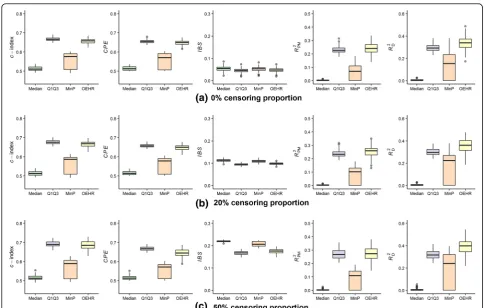
and the optimal equal-HR method under different par-ameter scenarios. Figures3,4, 5 examined the perform-ance of Cox models with a continuous covariate discretized by the four different discretization methods.

When (k1, k2, a) equaled (−2, 2, 0), the relationship between the continuous covariate and log(λ) was almost symmetric (censoring might cause mild asymmetry). The median method had the worst performance out of the four discretization methods (Fig.3). The cut-points found by the minP method had much larger simulation standard errors than the other methods (Table 1). The median values of cut-points selected by the minP method were 0.60 (Pc= 0%), 0.00 (Pc= 20%), and−0.76 (Pc= 50%), which also reflected the considerable variation. The minPmethod per-formed better than the median method, but worse than the optimal equal-HR method and the Q1Q3 method. In terms ofc-index,CPE,andIBS measures, using Q1Q3 values as cut-points was slightly better than the other methods in-cluding the optimal equal-HR method (Fig.3). As forRPM2 andRD2measures, the optimal equal-HR method had the better performance than the other three methods.

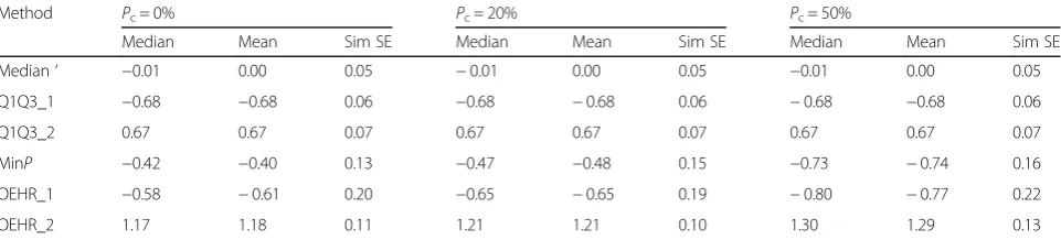
When (k1,k2,a) equaled (−8/5, 8/3, 1/2), the relation-ship between the continuous covariate and log(λ) was moderate asymmetric. The median value method had the worst performance among the four discretization

methods (Fig.4). In this case, the variation of cut-points found by the minP method was smaller than that in the symmetric situation (Table 2), and the minP method ranked the third regarding overall performance. The Q1Q3 method ranked the second. Overall, the optimal equal-HR method had the best performance out of the four methods. However, the advantage of the optimal equal-HR method over the Q1Q3 method was quite slight in terms ofc-index,CPE, andIBS.

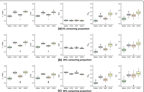
When (k1,k2,a) equaled (−4/3, 4, 1), the relationship between the continuous covariate and log(λ) was severe asymmetric. In this case, the optimal equal-HR method had an obvious advantage over the other three methods in terms of c-index, CPE, IBS, RPM2 andRD2 measures (Fig. 5). Quantitatively, the differences between the performance of the optimal equal-HR method and the Q1Q3 method were larger than those in the moderate situation under different censoring proportions. For example, comparing the optimal equal-HR method with the Q1Q3 method, the difference of their c-indexes changed from 0.008 (moderate asymmetric situation) to 0.043 (severe asymmetric situation) when the Pc was 0%. Therefore, when the relationship between the con-tinuous covariate and log(λ) was severe asymmetric, the optimal equal-HR method had much better Table 1Estimated cut-points when (k1,k2,a) equals (−2, 2, 0) in simulation data

Method Pc= 0% Pc= 20% Pc= 50%

Median Mean Sim SE Median Mean Sim SE Median Mean Sim SE

Median‘ −0.01 0.00 0.05 −0.01 0.00 0.05 −0.01 0.00 0.05

Q1Q3_1 −0.68 −0.68 0.06 −0.68 −0.68 0.06 −0.68 −0.68 0.06

Q1Q3_2 0.67 0.67 0.07 0.67 0.67 0.07 0.67 0.67 0.07

MinP 0.60 0.06 0.77 0.00 −0.02 0.84 −0.76 −0.01 1.03

OEHR_1 −0.90 −0.89 0.15 −0.93 −0.93 0.16 −1.02 −1.03 0.17

OEHR_2 0.90 0.90 0.15 0.94 0.93 0.15 1.01 1.03 0.17

Pc= censoring proportion; Sim SE = simulation standard error; Median‘= using the median value of the continuous covariate as a cut-point; Q1Q3 = using the upper and lower quartiles values as cut-points, Q1Q3_1 is the upper quartile value and Q1Q3_2 is the lower quantile value; MinP= the single cut-point minimum

p-value method with log-rank test; OHER = the optimal equal-HR method proposed in this study, OEHR_1 is the left estimated cut-point and OEHR_2 is the right estimated cut-point

Table 2Estimated cut-points when (k1,k2,a) equals (−8/5, 8/3, 1/2) in simulation data

Median_‘ ₋0.01 0.00 0.05 ₋0.01 0.00 0.05 ₋0.01 0.00 0.05

Q1Q3_1 ₋0.68 ₋0.68 0.06 ₋0.68 ₋0.68 0.06 ₋0.68 ₋0.68 0.06

Q1Q3_2 0.67 0.67 0.07 0.67 0.67 0.07 0.67 0.67 0.07

Min_P ₋0.42 ₋0.40 0.13 ₋0.47 ₋0.48 0.15 ₋0.73 ₋0.74 0.16

OEHR_1 ₋0.58 ₋0.61 0.20 ₋0.65 ₋0.65 0.19 ₋0.80 ₋0.77 0.22

OEHR_2 1.17 1.18 0.11 1.21 1.21 0.10 1.30 1.29 0.13

(7)

performance than the Q1Q3 method, the median split method and the minPmethod.

According to the above results, we could get the following messages

The Q1Q3 method and the optimal equal-HR

method have comparable good performance when the U-shaped relationship between the continuous

covariate and log(λ) is almost symmetric. As the U-shaped relationship becomes asymmetric, the optimal equal-HR method has better perform-ance than the Q1Q3 method.

The median method and the minPmethod are

not recommended when there exist U-shaped relationships between the continuous covariates and log(λ) since these two methods don’t have good performance under all simulation scenarios.

Table 3Estimated cut-points when (k1,k2,a) equals (−4/3, 4, 1) in simulation data

Median‘ −0.01 0.00 0.05 −0.01 0.00 0.05 −0.01 0.00 0.05

Q1Q3_1 −0.68 −0.68 0.06 −0.68 −0.68 0.06 −0.68 −0.68 0.06

Q1Q3_2 0.67 0.67 0.07 0.67 0.67 0.07 0.67 0.67 0.07

MinP −0.08 −0.08 0.15 −0.19 −0.20 0.17 −0.51 −0.51 0.20

OEHR_1 −0.41 −0.39 0.23 −0.45 −0.46 0.24 −0.60 −0.59 0.26

OEHR_2 1.49 1.49 0.08 1.51 1.52 0.08 1.55 1.55 0.10

p-value method with log-rank test; OHER = the optimal equal-HR method proposed in this study, OEHR_1 is the left estimated cut-point and OEHR_2 is the right estimated cut-point

(8)

Results of the application on a real dataset

Small cell lung cancer (SCLC) is a subtype of lung cancer with terrible survival outcomes. It is characterized by high invasiveness, high growth fraction, and poor prognosis. Fibrinogen (FIB), a protein that is synthesized by the liver and has a blood coagulation function, plays an important role in the pathogenesis of cardiovascular diseases. The reference range of FIB is 2–4 g/L. Several studies have found that the higher FIB level was associated with shorter overall survival (OS) [32–34]. Some authors used the median value of FIB as a cut-point of low and high FIB level [32, 33], when some others used the upper limit of the reference range as a cut-point [34].

We used the data of 275 patients with SCLC in the First Affiliated Hospital of Guangzhou Medical University from January 2009 to December 2013 [35]. FIB ranged from 0.98 to 9.23 g/L (mean ± SD: 4.78 ± 1.56 g/L). There were 235 events (deaths) during the study period. The OS ranged from 0 to 86 months (median: 12 months), and the 1-, 2-year OS rates were 50 and 21%, respectively.

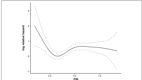
First, the effect of FIB on log relative hazards was curved by a Cox model with P-splines. The U-shaped graph (Fig. 6) indicated that the patients with low and

high FIB values might have a higher risk of deaths when compared to those with FIB values in the median range. It meant that the data was suitable to apply the optimal equal-HR method. Then, the median method, the Q1Q3 method, the minP method and the optimal equal-HR method were applied in the data.

Table 4 showed the cut-points found by the four methods. The median method selected 4.52 as a cut-point, the Q1Q3 method selected two cut-points at 3.59 and 5.84, the minP method selected 4.02, and the optimal equal-HR method chose 2.62 and 4.06 as cut-points. The cut-points of the optimal equal-HR method were closest to the reference range of FIB (2–4 g/L).

Four Cox models were fitted with the discretized FIB variable. Reference levels of the discretized FIB were < 4.52 for the median method, 3.59–5.84 for the Q1Q3 method, < 4.02 for the minP method, and 2.62–4.06 for the optimal equal-HR method. In the Cox model with the FIB discretized by the optimal equal-HR method, both low FIB level (< 2.62) and high FIB level (> 4.06 g/ L) had adverse effects (P-value < 0.05) on survival outcomes, while it was not statistically significant using the Q1Q3 method.

(9)

Table 5 illustrated the performance of different esti-mated cut-points in Cox models. 100-times five-fold cross-validation was used to obtain accurate estimations of the performance. The cut-points estimated by the op-timal equal-HR method had the best performance in dis-crimination power and overall performance (explained variance) in terms of c-index, CPE, IBS, RPM2 and RD2 measures. In conclusion, the optimal equal-HR method provided clinical meaningful and well-performed cut-points in the case study.

Discussion

In this study, we propose the optimal equal-HR method to discretize a continuous predictor when the relationship between the predictor and log(λ) is U-shaped. We demon-strate the results of the Monte Carlo simulation study with different censoring proportions, baseline functions, and relationship curves. When the relationship between the predictor and log(λ) is symmetric (peak asymmetry factor equals 1), it’s hard to describe whether the Q1Q3 method or the optimal equal-HR method has better performance. At a first look, it surprises us a little that the Q1Q3 method has such good performance. The two possible reasons for

the good performance of the Q1Q3 method are as follows. One is that under the symmetric scenario, the Q1Q3 method finds two cut-points with close log(λ) values, which conforms to the principle of the optimal equal-HR method. The other is that the Q1Q3 method divides samples into three groups with 1:2:1 sample sizes while the optimal equal-HR method might result in more unbalanced ratios of sample sizes. When the relationship becomes asymmet-ric, which is common in practice, the optimal equal-HR method has better performance than the Q1Q3 method, the median method, and the minPmethod. The SCLC case study has also proved that the cut-points selects by the op-timal equal-HR method have more plausible biological sense and better model performance in the asymmetric situation.

We have only used the optimal equal-HR method under univariate Cox regression models in this study. The effect of continuous predictors on survival outcome might be influenced by other confounding variables. Therefore, it is important to include those variables in Cox models. Mazumber, et al [36] suggested that when we add a new categorical predictor to an existing multi-variate model, searching the cut-points for the new

(10)

variable should be done in the existing multivariate setting. The optimal equal-HR method could easily extend to multivariate Cox models after the selection of confounding variables is made depend on the ground of clinical and epidemiological understandings. As mentioned before, the optimal equal-HR method includes two main steps: (1). the graphical diagnostic plots, (2). find two optimal cut-points. The optimal equal-HR method could be applied in a multi-variate context as follows. First, the diagnostic plots and estimated log relative hazards could be obtained from a multivariate Cox regression model with penalized B-splines, which means the functional form for the interested ate is determined under the condition that all other covari-ates remain constant. Then, the optimal cut-points of the interested covariate will be the cut-points in the multivari-ate Cox regression model with minimumAICvalue. Add-itionally, the simulation results in Additional file 1: Tables

S4 and S5 showed that applying our method in a multivari-ate context will provide more reasonable estimmultivari-ates of both optimal cut-points (smaller variations) and Cox regression coefficients (closer to the true regression coefficients) than that in a univariate context if the survival outcomes are truly affected by other covariates. Nevertheless, the R pack-age ‘CutpointsOEHR’ already supports seeking optimal cut-points in a multivariate context. However, when there are two or more covariates that need to be categorized, the implementation of the optimal equal-HR method remains to be addressed in further studies.

Other researchers have also proposed different ways to find two optimal cut-points. Camp, et al [37] developed X-Tile, a bio-informatics tool to find optimal cut-points, which is widely used in genetic data. The X-Tile accesses all combinations of two cut-points and selects the one with the highest log-rankχ2value as the optimal pair of cut-points.

Fig. 6The relationship between FIB and log(λ) in small cell lung cancer data. The black solid line is the estimated log relative hazard of FIB by Cox model withP-spline, the grey dashed lines present 95% confidence interval of the estimated log relative hazard

Table 4Estimated cut-points of FIB and results of Cox models with discretized FIB

Method cut-point1 cut-point2 β1 HR1 P-value1 β2 HR2 p-value2

Median 4.52 – 0.43 1.54 0.002 – – –

Q1Q3 3.59 5.84 −0.33 0.72 0.059 0.17 1.18 0.295

minP 4.02 – 0.46 1.59 0.001 – – –

OEHR 2.62 4.06 1.08 2.94 < 0.001 0.61 1.83 < 0.001

Median denotes using the median value of the continuous covariate as a cut-point. Q1Q3 denotes using the upper and lower quartiles values as cut-points. MinP

(11)

Compared to the X-Tile, the optimal equal-HR method finds two cut-points with approximately equal log(λ) values, which is based on the underlying idea of classifying high-risk or low-risk population according to their log rela-tive hazards. In this way, the optimal equal-HR method might provide more clinical valuable cut-points than the X-tile, offer clues for finding reasonable reference ranges, and reduce the number of computer operations. We might expect a better prediction performance if we allow different hazard values for two cut-points. Therefore, it is possible to improve our strategy with a trade-off between prediction performance and clinical meaning in further studies.

There are more works to be done in the future to generalize the utilization of the optimal equal-HR method: (1) This method uses Cox models with penalized B-splines to curve U-shaped relationships, which requires covariates to satisfy the proportional hazard (PH) assumption. There-fore, further studies are needed to release the PH assump-tion. (2) We focus on the U-shaped relationships between covariates and log relative hazards in this study. The modifi-cation and applimodifi-cation of the optimal equal-HR method to other types of nonlinear relationships remain to be explored. It is important to remember that lots of literature have proved that discretization will inevitably result in infor-mation loss [38–40]. This study did not encourage researchers to blindly discretize continuous independent variables when fitting Cox models. The decision to discretize a continuous covariate should be cautiously made by the investigators based on clinical needs. What’s more, the precondition of our method is the U-shaped relationship between an interested continuous covariate and survival outcomes. We recommend using the graphical diagnostic plots, which are based on Cox models with penalized B-splines, to visualize the data and determine whether there exists U-shaped relation-ships or not. Besides the graphical diagnostic plots, formal tests, such as the two-lines test [41], could also facilitate the judgement of U-shaped relationships.

Conclusions

In general, the optimal equal-HR method proposed in our study offers researchers a solution to find optimal cut-points of continuous predictors that have U-shaped

relationships with log(λ) in survival analysis. If researchers have decided to discretize a continuous predictor in Cox models, we highly advise them to explore the relationships between continuous predictors and survival outcomes firstly. When the relationships are U shapes, of which the majority are asymmetric in real-world data, the optimal equal-HR method is recommended to find two optimal cut-points. In addition, an R package called ‘ Cutpoint-sOEHR’has been developed for easy use of this method-ology in practice.

Additional file

Additional file 1:Table S1.Comparison of the cut-points selected by

the optimal equal-HR method usingAICandBICin simulated datasets when (k1,k2,a) equals (−2, 2, 0).Table S2.Comparison of the cut-points selected by the optimal equal-HR method usingAICandBICin simulated datasets when (k1,k2,a) equals (−8/5, 8/3, 1/2).Table S3.Comparison of the cut-points selected by the optimal equal-HR method usingAICand BICin simulated datasets when (k1,k2,a) equals (−4/3, 4, 1).Table S4. The estimated cut-pointsaby the multivariate and univariate approaches of the optimal equal-HR method.Table S5.The estimated Cox regression coefficientsaof covariates discretized by the multivariate and univariate approaches of the optimal equal-HR method.Figure S1.Predictive per-formance of estimated cut-points when sample sizes are 250.Figure S2.

Predictive performance of estimated cut-points when sample sizes range from 100 to 500 (DOCX 441 kb)

Abbreviations

AIC:Akaike Information Criterion; CPE: Concordance probability estimate; HR: Hazard ratio; IBS: Integrated brier score; Min_P: Minimum_p-value approach to find optimal cut-points;Pc: Censoring proportion; Q1Q3: Upper quantile and lower quantile values; SE: Standard error

Acknowledgments

We would like to thanks Hui Pan for giving access to the small cell lung cancer data for this study.

Funding

This study was supported by the Natural Science Foundation of Guangdong Province, China (2016A030313365), the Science and Technology Program of Guangdong Province, China (2014A020212713) and the National Natural Science Foundation of China (NSFC, 81773545) in the design of the study, simulation and analysis of data and in writing the manuscript.

Availability of data and materials

The main codes of the simulation study are provided on the Supplementary Material. The small cell lung cancer data applied in this study are available from Hui Pan but restrictions apply to the availability of these data, which were used under license for the current study but not publicly available. The small cell lung cancer data are however available from the authors upon reasonable request and with permission of Hui Pan.

Table 5Performance of different estimated cut-points of FIB in Cox models by 100-times five-fold cross-validation

Performance measures (mean ± standard error)

Method c-index CPE IBS RPM2 RD2

Median 0.552 ± 0.006 0.554 ± 0.005 0.141 ± 0.004 0.037 ± 0.009 0.065 ± 0.017

Q1Q3 0.555 ± 0.010 0.557 ± 0.009 0.141 ± 0.005 0.040 ± 0.012 0.036 ± 0.015

minP 0.538 ± 0.009 0.543 ± 0.008 0.142 ± 0.004 0.027 ± 0.010 0.047 ± 0.019

OEHR 0.569 ± 0.010 0.572 ± 0.009 0.138 ± 0.006 0.069 ± 0.015 0.076 ± 0.020

Median denotes using the median value of the continuous covariate as a cut-point. Q1Q3 denotes using the upper and lower quartiles values as cut-points. MinP

(12)

Authors’contributions

JZ, YC, JH and XH conceived and designed the study. All authors have made contributions to the development of the optimal equal-HR method. YC per-formed the simulations and made the data analyses. YC and GM drafted the manuscript. All authors interpreted the study. JZ supervised YC at all stages. All authors read and approved the final manuscript.

Ethics approval and consent to participate

The small cell lung cancer data from Hui Pan’s published article [35] was used in the manuscript as an example. The ethical statement in the published article is as follows: This retrospective study was approved by the Institutional Review Board of GMUFAH and Cancer Center of Guangzhou Medical University (GMUCC) (GMUFAH approval No: 2017–03; GMUCC approval No: P2017_–001).

Consent for publication

The manuscript does not contain any individual person’s data.

Competing interests

The authors declare that they have no competing interests.

Publisher’s Note

Springer Nature remains neutral with regard to jurisdictional claims in published maps and institutional affiliations.

Author details

1_{Department of Medical Statistics and Epidemiology, School of Public Health,}

Sun Yat-sen University, Guangzhou 510080, China.2National Engineering Laboratory for Internet Medical Systems and Applications, the First Affiliated Hospital of Zhengzhou University, Zhengzhou 450052, Henan, China.

Received: 19 December 2018 Accepted: 22 April 2019

References

1. Cox DR. Regression models and life-tables. J R Stat Soc. 1972;34(2):187–220. 2. Calabrese EJ, Baldwin LA. U-shaped dose-responses in biology, toxicology,

and public health. Annu Rev Public Health. 2001;22:15_–33.

3. Hamer M, Stamatakis E. U-shaped association between body mass index and psychological distress in a population sample of 114,218 British adults. Mayo Clin Proc. 2017;92(12):1865–6.

4. Ervasti J, Kivimaki M, Head J, Goldberg M, Airagnes G, Pentti J, Oksanen T, Salo P, Suominen S, Jokela M, et al. Sickness absence diagnoses among abstainers, low-risk drinkers and at-risk drinkers: consideration of the U-shaped association between alcohol use and sickness absence in four cohort studies. Addiction. 2018;113(9):1633_–42.

5. Du X, Zhu B, Hu G, Mao W, Wang S, Zhang H, Wang F, Shi Z. U-shape association between white blood cell count and the risk of diabetes in young Chinese adults. Diabet Med. 2009;26(10):955–60.

6. Govindarajulu US, Spiegelman D, Thurston SW, Ganguli B, Eisen EA. Comparing smoothing techniques in Cox models for exposure-response relationships. Stat Med. 2007;26(20):3735–52.

7. Roshani D, Ghaderi E. Comparing smoothing techniques for fitting the nonlinear effect of covariate in Cox models. Acta Inform Med. 2016;24(1):38_–41. 8. Therneau TM, Grambsch PM. Modeling survival data: extending the Cox

model. New York: Springer; 2000.

9. Bouwmeester W, Zuithoff NP, Mallett S, Geerlings MI, Vergouwe Y, Steyerberg EW, Altman DG, Moons KG. Reporting and methods in clinical prediction research: a systematic review. PLoS Med. 2012;9(5):1–12. 10. Mabikwa OV, Greenwood DC, Baxter PD, Fleming SJ. Assessing the

reporting of categorised quantitative variables in observational epidemiological studies. BMC Health Serv Res. 2017;17(1):201. 11. Budczies J, Klauschen F, Sinn BV, Gyorffy B, Schmitt WD, Darb-Esfahani S,

Denkert C. Cutoff finder: a comprehensive and straightforward web application enabling rapid biomarker cutoff optimization. PLoS One. 2012;7(12):e51862. 12. Raghavan R, Ashour FS, Bailey R. A review of cutoffs for nutritional

biomarkers. Adv Nutr. 2016;7(1):112–20.

13. Prince Nelson SL, Ramakrishnan V, Nietert PJ, Kamen DL, Ramos PS, Wolf BJ. An evaluation of common methods for dichotomization of continuous variables to discriminate disease status. Commun Stat Theory Methods. 2017;46(21):10823–34.

14. Knuppel L, Hermsen O. Median split, k-group split, and optimality in continuous populations. Asta-Adv Stat Anal. 2010;94(1):53_–74.

15. Iacobucci D, Posavac SS, Kardes FR, Schneider MJ, Popovich DL. Toward a more nuanced understanding of the statistical properties of a median split. J Consum Psychol. 2015;25(4):652–65.

16. Miller R, Siegmund D. Maximally selected chi square statistics. Biometrics. 1982;38(4):1011–6.

17. Mazumdar M, Glassman JR. Categorizing a prognostic variable: review of methods, code for easy implementation and applications to decision-making about cancer treatments. Stat Med. 2000;19(1):113_–32. 18. Thinggaard M, Jacobsen R, Jeune B, Martinussen T, Christensen K. Is the

relationship between BMI and mortality increasingly U-shaped with advancing age? A 10-year follow-up of persons aged 70-95 years. J Gerontol Ser A-Biol Sci Med Sci. 2010;65(5):526_–31.

19. Gamel JW, McLean IW. A method for determining the optimum transform for covariates of the Cox model with application to 3680 cases of intraocular melanoma. Comput Biomed Res. 1988;21(5):471–7. 20. Klein JP, Wu JT. Discretizing a continuous covariate in survival studies.

Handbook Stat. 2003;23(03):27–42.

21. Molinari N, Daures JP, Durand JF. Regression splines for threshold selection in survival data analysis. Stat Med. 2001;20(2):237–47.

22. Eilers PHC, Marx BD. Flexible smoothing with B-splines and penalties. In: Statistical Science, vol. 1996; 1996. p. 89–121.

23. Meira-Machado L, Cadarso-Suarez C, Gude F, Araujo A. smoothHR: an R package for pointwise nonparametric estimation of hazard ratio curves of continuous predictors. Comput Math Methods Med. 2013;2013:745742. 24. Bender R, Augustin T, Blettner M. Generating survival times to simulate Cox

proportional hazards models. Stat Med. 2005;24(11):1713_–23.

25. Foley JP, Dorsey JG. Equations for calculation of chromatographic figures of merit for ideal and skewed peaks. Anal Chem. 1983;55(4):730_–7.

26. Harrell FE Jr, Lee KL, Califf RM, Pryor DB, Rosati RA. Regression modelling strategies for improved prognostic prediction. Stat Med. 1984;3(2):143_–52. 27. Gonen M, Heller G. Concordance probability and discriminatory power in

proportional hazards regression. Biometrika. 2005;92(4):965_–70.

28. Graf E, Schmoor C, Sauerbrei W, Schumacher M. Assessment and comparison of prognostic classification schemes for survival data. Stat Med. 1999;18(17–18): 2529–45.

29. Tawn JA. Measures of dependence for censored survival data. Biometrika. 1988;75(3):525–34.

30. Royston P, Sauerbrei W. A new measure of prognostic separation in survival data. Stat Med. 2004;23(5):723–48.

31. Faraggi D, Simon R. A simulation study of cross-validation for selecting an optimal cutpoint in univariate survival analysis. Stat Med. 1996;15(20):2203–13. 32. Ferrigno D, Buccheri G, Ricca I. Prognostic significance of blood coagulation

tests in lung cancer. Eur Respir J. 2001;17(4):667–73.

33. Tas F, Kilic L, Serilmez M, Keskin S, Sen F, Duranyildiz D. Clinical and prognostic significance of coagulation assays in lung cancer. Respir Med. 2013;107(3):451–7.

34. Zhu LR, Li J, Chen P, Jiang Q, Tang XP. Clinical significance of plasma fibrinogen and D-dimer in predicting the chemotherapy efficacy and prognosis for small cell lung cancer patients. Clin Transl Oncol. 2016;18(2):178–88.

35. Pan H, Shi X, Xiao D, He J, Zhang Y, Liang W, Zhao Z, Guo Z, Zou X, Zhang J, et al. Nomogram prediction for the survival of the patients with small cell lung cancer. J Thorac Dis. 2017;9(3):507_–18.

36. Mazumdar M, Smith A, Bacik J. Methods for categorizing a prognostic variable in a multivariable setting. Stat Med. 2003;22(4):559–71. 37. Camp RL, Dolled-Filhart M, Rimm DL. X-tile: a new bio-informatics tool for

biomarker assessment and outcome-based cut-point optimization. Clin Cancer Res. 2004;10(21):7252–9.

38. Royston P, Altman DG, Sauerbrei W. Dichotomizing continuous predictors in multiple regression: a bad idea. Stat Med. 2006;25(1):127–41.

39. Altman DG, Royston P. The cost of dichotomising continuous variables. BMJ. 2006;332(7549):1080.

40. Barnwell-Menard JL, Li Q, Cohen AA. Effects of categorization method, regression type, and variable distribution on the inflation of type-I error rate when categorizing a confounding variable. Stat Med. 2015;34(6):936_–49. 41. Simonsohn U. Two lines: a valid alternative to the invalid testing of