Winter and summer
differences in probability
of fish encounter (spatial overlap) with MHK devices
Haley Viehman
#1, Tyler Boucher
*2, Anna Redden
#3#Acadia Centre for Estuarine Research, Acadia University
23 Westwood Ave., Wolfville, Nova Scotia B4P 2R6, Canada
*Fundy Ocean Research Center for Energy PO Box 2573, Halifax, Nova Scotia B3J 1V7, Canada
Abstract—The likelihood of fish encountering an MHK device, and therefore the risk posed to fish, depends largely on the natural distribution of fish at tidal energy development sites. In temperate locations, such as the Bay of Fundy, seasonal changes in the environment and fish assemblage may alter the likelihood of fish encounters with MHK devices. We examined two one-month hydroacoustic datasets collected in winter 2015 and summer 2016 by an upward-facing echosounder deployed at the Fundy Ocean Research Center for Energy test site in the Minas Passage. Fish density was higher and less variable in winter than in summer, likely due to the presence of migratory vs. overwintering fish. The vertical distribution of fish varied with sample period, diel stage, and tidal stage. The proportion of fish at MHK device depth was greater, but more variable, in summer than in winter. Encounter probability, or potential for spatial overlap of fish with an MHK device, was < 0.002 for winter and summer vertical distributions. More information on the distribution of fish (horizontal and vertical), species present, fish sensory and locomotory abilities, and nearfield behaviours in response to MHK devices is needed to improve our understanding of likely device effects on fish.
Keywords—Fish, encounter risk, MHK, hydroacoustics, Bay of Fundy, FORCE
I. INTRODUCTION
The effects of marine hydrokinetic (MHK) devices on fish are generally unknown, but of high concern to industry, regulators, the scientific community, fishers and other stakeholders. To address this knowledge gap, the Fundy Ocean Research Center for Energy (FORCE) developed a series of marine sensor platforms to monitor physical and biological characteristics of the test site, where multiple MHK technologies will be deployed in coming years.
The FORCE test site is in the Minas Passage of the Bay of Fundy, where tidal range reaches 13 m and current speeds can exceed 5 m·s-1 [1]. The fish assemblage of this region changes seasonally [2]. Differences in fish assemblage and species behaviour with temperature means the risk MHK devices pose to fish will also vary seasonally. Depth preferences and vertical migration patterns vary with species and life stage of fish, so the likelihood of physical overlap with a fixed-depth MHK device will change with the fish assemblage. Additionally, temperature-related changes in physiology and behaviour alter the likelihood of fish interacting with an MHK device. For
example, striped bass were recently found to be present in the passage near year-round, but with reduced diel vertical migration during periods of very low temperatures [3].
The goal of this project was to compare the pre-device density and vertical distribution of fish at the FORCE site in winter 2015 and summer 2016 and consider the implications for the likelihood of fish interactions with a Cape Sharp Tidal MHK device (OpenHydro). This device spans 0-20 m above the sea floor and was installed in November 2016. We analysed hydroacoustic data collected at the FORCE site in winter and summer months to examine natural differences in (1) overall fish density, (2) fish vertical distribution, and (3) the proportion of fish at device depth, with respect to tide, diel stage, and time of year. This information was used to calculate the likelihood of spatial overlap of fish with an MHK device, a basic probability of encounter model.
II. METHODS
A. Data Collection
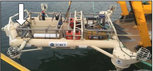
Hydroacoustic data were collected with an upward-facing ASL Environmental Sciences Acoustic Zooplankton and Fish Profiler (AZFP), mounted approximately 1.5 m above the sea floor on the FAST-1 bottom platform (Fig. 1).
Fig. 1 FAST-1 sensor platform developed by FORCE and deployed at the FORCE test site. White arrow indicates location of AZFP transducer.
Photo credit: Tyler Boucher.
The AZFP utilized a 125 kHz, 8° (half-power beam angle) circular transducer, which operated at a 300 μs pulse duration and ping rate of 1 Hz. Current speed and water temperature were recorded for 10 minutes every half hour by a Nortek
SPECIAL ISSUE OF THE TWELFTH EUROPEAN WAVE AND TIDAL ENERGY CONFERENCE, 27 SEPTEMBER - 1 AUGUST 2017, CORK, IRELAND
©EWTEC 2017. THIS IS AN OPEN ACCESS ARTICLE DISTRIBUTED UNDER THE TERMS OF THE CREATIVE COMMONS ATTRIBUTION 4.0 LICENCE (CC BY
h p://creativecommons.org/licenses/by/4.0/). UNRESTRICTED USE (INCLUDING COMMERCIAL), DISTRIBUTION AND REPRODUCTION IS PERMITTED PROVIDED THAT CREDIT IS GIVEN TO THE ORIGINAL AUTHOR(S) OF THE WORK, INCLUDING A URI OR HYPERLINK TO THE WORK, THIS PUBLIC LICENSE AND A COPYRIGHT NOTICE.
Signature 500 Acoustic Doppler Current Profiler (ADCP), also mounted on the platform. The platform was deployed at the FORCE test site for approximately one-month intervals. The first deployment spanned 8 December 2015 to 5 January 2016 (the “winter” dataset) and the second deployment was from 17 June to 13 July 2016 (the “summer” dataset).
The platform was deployed at the south-western corner of the FORCE test area in winter, and in summer, at a site nearer to the Cape Sharp Tidal MHK device location (site D, Fig. 2). Both sites are on a volcanic plateau formation that extends into Minas Passage, the 5.5-km-wide connection between Minas Basin and Minas Channel. The sites were approximately 1 km apart and experienced similar environmental conditions, including current velocity (mid-water-column current speed exceeding 4 m∙s-1 at peak flood tide and 3 m∙s-1 at peak ebb tide) and depth range (spring tide depths of 33 to 45 m at the winter site, 30 to 43 m at the summer site). Temperatures ranged from 5.4°C to 8.4°C during the winter deployment, and from 9.9°C to 13.6°C during the summer deployment.
B. Data Processing
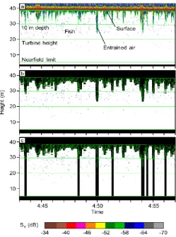
Hydroacoustic data were processed in Echoview® software (8.0, Myriax, Hobart, Australia). Steps included applying calibration constants, setting a -60 dB target strength threshold to remove most non-fish targets and fish under a few cm in length [5-11], excluding data that has acoustic interference from the ADCP, and removing acoustic signal from the acoustic nearfield and from entrained air (Fig. 3).
Calibration of the echosounder was carried out by the manufacturer prior to the December 2015 deployment. A second calibration conducted in January 2017 revealed the echosounder had drifted by several dB over that time. The majority of this drift appears to have occurred after the June 2016 deployment: examination of surface backscatter from the December 2015 and June 2016 deployments showed a drop of approximately 2 dB from December to June, which was within the error range of the manufacturer’s calibration. The
December and June datasets are therefore comparable using the factory calibration settings, but this difference should be kept in mind when interpreting results.
A layer of entrained air was almost always present near the surface, and at peak flows, turbulence frequently drew air to depths near the seafloor. Entrained air is a common issue at tidal energy sites [12-14]. Because air is a strong acoustic target, any fish that may have been within the entrained air layer were not detectable. Entrained air was removed from the data with a series of steps in Echoview® that used a modified bottom-detection algorithm to isolate the air layer (Fig. 3a), then expanded its boundaries slightly to remove any fringe signal that was not encompassed by the line (Fig. 3b).
Due to the high prevalence of entrained air at 0-10 m depth, the subsequent analyses were limited to depths greater than 10 m. Additionally, any pings in which entrained air surpassed 10 m depth were entirely excluded from the dataset (Fig. 3c). This resulted in more pings lost during periods of high flow (i.e., mid-tide; Fig. 4a), particularly during the flood tide, which was more turbulent. However, excluding entire pings improved comparability of values obtained from throughout the water column.
Fig. 2 Study site with deployment locations. Lower panel shows site bathymetry and proposed MHK device sites (A-D) at the FORCE test site. Location of the FAST-1 platform in winter 2015 indicated by , summer by
. Upper panel maps made in QGIS with data obtained from GeoGratis
Canada and bathymetry data from [4]. Lower panel map produced by Seaforth Geosurveys, Inc.
Fig. 3 Example of volume backscatter (SV) data collected from
4:43 to 4:57 UTC on 9 December 2015. (a) Raw data, showing entrained air and lines in data processing. (b) Processed data, with entrained air removed.
C. Data Analysis
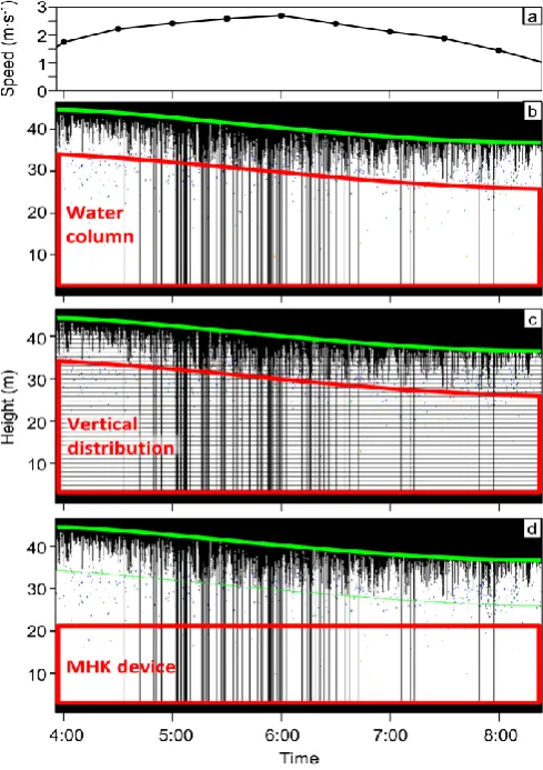
Analysis was divided into three parts: (1) analysis of fish backscatter from the whole water column (Fig. 4b), (2) inspection of the vertical distribution of backscatter (Fig. 4c), and (3) comparison of backscatter from the depths spanned by the proposed MHK device to that from the water column (Fig. 4d).
Hydroacoustic data were first split into segments according to tidal (ebb or flood) and diel (day or night) stages. Slack tides were defined as periods when mid-water-column current speed was less than 1 m∙s-1. The rise and fall in current speed was slightly asymmetrical (Fig. 4a). Low slack tide averaged 70 min (9.4 min standard deviation) in length while high slack tide averaged 44 min (7.1 min standard deviation). Slack tides were then omitted from analyses in order to focus on ebb and flood tides, when an MHK turbine would be rotating (depending on cut-in speed) and thus a potentially greater risk to fish. Periods of dusk and dawn were then defined as the hours centred at sunrise and sunset, and were also excluded in order to avoid likely periods of vertical fish migration that could confound
analysis of vertical distribution. The remaining data segments were classified by tidal stage and diel stage, and were treated as separate samples. Any of these samples missing more than half of their data points due to entrained air were omitted from analyses.
Further analysis required partitioning the water column in three different ways (Fig. 4). The water column used in analyses was limited to the portion between the acoustic nearfield (3.2 m height above the sea floor) and the 10-m depth line (Fig. 4b). Assessing the vertical distribution of backscatter required splitting this analysis region into 1-m-deep layers measured upward from the face of the transducer (Fig. 4c). To compare MHK device depth to the rest of the water column, the analysis region was split at proposed device height (20 m above the seafloor; Fig. 4d). From here onward, “water column” refers to the portion of the true water column which we were able to analyse.
The acoustic metrics exported from these portions of the water column for each time segment were mean volume backscatter and the area backscattering coefficient. Volume backscatter, SV, is the amount of acoustic energy scattered by a unit volume of water and is a rough proxy for fish density [15, 16]. SV is expressed logarithmically in units of decibels (dB re 1 m-1) or in the linear domain as sv, with units of m2·m-3. Mean SV was calculated for the entire (analysed) water column to examine general differences in fish density with respect to tidal stage, diel stage, and sampling period. The area backscattering coefficient, sa, is sv integrated over a given layer of the water column (units of m2·m-2), and so is also a proxy of fish density. sa was used to calculate the proportion of acoustic backscatter contributed by each 1-m layer of water and from the depths spanned by the proposed MHK device.
Statistical analyses were carried out in R (3.3.1, R Core Team, Vienna, Austria). Differences in water column SV and the proportion of backscatter from the MHK device depths related to tidal stage (ebb or flood), diel stage (day or night), and sampling period (winter or summer) were examined using analysis of variance (ANOVA) tests with a significance level of 0.05. Comparisons between factor groups found to have significant effects were carried out with Tukey-type multiple comparisons. Nonparametric versions of these tests
(permutation ANOVA, nonparametric Tukey-type
comparisons) were used for water column SV data, which did not meet the assumptions of normality. The linear form of SV (𝑠𝑣= 10𝑆𝑉⁄10) was used in significance testing and to calculate summary statistics.
The probability that fish might encounter an MHK device was estimated as the probability of spatial overlap with the device under three fish distribution scenarios: (1) uniform vertical distribution; (2) winter vertical distribution; and (3) summer vertical distribution. For this exploratory exercise, fish horizontal distribution (across the breadth of the passage) was assumed uniform, and the proportion of backscatter at turbine depth was assumed equivalent to the proportion of fish at that depth range (i.e., acoustic properties were assumed the same for all fish). Under scenario 1, the probability of encounter was simply the cross-sectional area of the turbine divided by that of Fig. 4 Data from one ebb tide from 3:56 to 8:23 UTC on 9 December
2015. (a) Current speed from 16-17 m above the sea floor. (b-d) The three water column partitions used in analysis: (b) entire water column, defined as
the passage. For scenarios 2 and 3, the probability was the proportion of passage cross-section spanned by the turbine’s width multiplied by the proportion of fish at turbine depth in winter and summer (the median proportion of backscatter at turbine depth). The passage cross-sectional area at site D (Fig. 2) was estimated as 338,814 m2 at mean tidal height, using bathymetry data in [4] and Quantum GIS open source software package (2.18.7, QGIS Development Team). The area of a single Cape Sharp Tidal device was approximated as 320 m2 (16 m width x 20 m height), and the area of the vertical slice of the passage spanned by the turbine was 592 m2 (16 m width x 37 m depth).
III.RESULTS
After data processing, 51 flood tides and 64 ebb tides remained for analysis in the winter dataset, and 66 flood tides and 71 ebb tides remained in the summer dataset (Fig. 5, full page display). In the winter dataset, fish were almost always present, mainly as individuals spread out in the water column, though small, compact aggregations were also present during the day. In the summer dataset, there were long spans of empty water column or water column interspersed with a few individual traces, punctuated occasionally during the day by loose or compact aggregations of fish. Aggregations of fish were not observed at night in either dataset. During calm periods with little entrained air, fish could often be seen in the upper 10 m of water that were excluded from analyses (Fig. 3, Fig. 4), which should be kept in mind while interpreting results.
A. Water column fish density
The water column mean SV (index of fish density) was significantly higher in the winter dataset than in the summer one, by approximately 8 dB (Fig. 6a). The median (IQR) SV in winter was -84.2 dB (-85.6, -83.1) and in summer was -92.7 dB (-94.9, -88.7). Tidal and diel stage were not found to significantly affect water column mean SV, but it is worth noting that in the summer, mean SV was noticeably lower at night than during the day (Fig 6b).
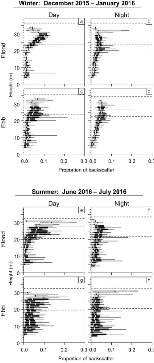
Fig. 7 Vertical distribution of area backscatter during time periods of interest, from the winter (a-d) and summer (e-h) datasets. Thick vertical lines indicate median, boxes encompass the interquartile range, and whiskers
span the 10th to 90th percentiles of each 1-m layer of the water column. Grey boxes indicate sample sizes less than 10. Horizontal dashed lines are
the minimum and maximum height of the analysed water column (which extended upward to 10 m below the true surface) for the duration of each
time period. Height is measured upward from the sea floor. Fig. 6 Water column mean volume backscatter, SV (proportional to fish
density). (a) Winter vs. summer. (b) Day vs. night in winter and summer. Sample sizes are shown at top. Letters indicate groups with significantly
different means (a highest, b lowest), where tested. White diamonds are means, horizontal bars are medians, boxes span 25th to 75th percentiles, and
B. Vertical distribution
Vertical distributions were generally ‘top-heavy’ regardless of sample period, tidal stage, or diel stage. Backscatter was typically strongest in the upper layers that were analysed, though a secondary increase was present at times in the lowest layers (Fig. 7). Differences in vertical distribution related to tidal stage, diel stage, and sampling period were also apparent. Diel differences were particularly noticeable in the winter dataset: during the day (Fig. 7a,c), backscatter was strongest in the upper layers of the water column, with a minimum centred at approximately 15 m above the sea floor. At night (Fig. 7b,d), backscatter was distributed more evenly across depths, increasing from the lowest layers to approximately 20 m height above the sea floor, and remaining similar or decreasing slightly in higher layers. In the summer dataset (Fig. 7e-h), higher variability in the backscatter within each layer made vertical distributions less distinct than in winter, and indicated vertical distribution was less consistent over time. In the summer, a diel difference in vertical distribution similar to that of winter was apparent for flood tide (Fig. 7e,f) but not for ebb tide (Fig. 7g,h). During the ebb tide, backscatter was more uniformly spread across layers during the day and slightly higher in the uppermost layers (though variability was high; Fig. 7g); at night, most of the backscatter was contributed by the upper- and lower-most layers (Fig. 7h).
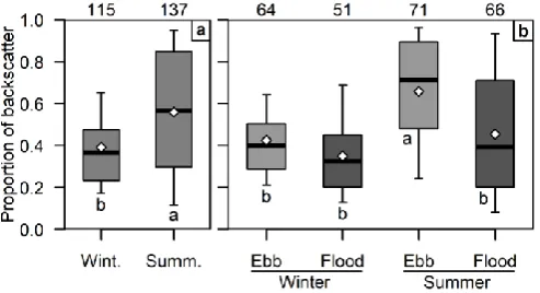
C. Fish at MHK device depth
The proportion of fish backscatter from the depths spanned by the MHK device (0-20 m height) was significantly higher in summer than in winter (median and IQR for winter: 0.365, 0.232-0.476; summer: 0.566, 0.297-0.848; Fig. 8a). The interaction of sample time with tidal stage was also significant: in winter, flood and ebb tide had similar proportions of backscatter at device depth (flood: 0.325, 0.202-0.451; ebb: 0.401, 0.288-0.504), while in summer ebb-tide proportions were higher than flood (flood: 0.393, 0.201-0.710; ebb: 0.714, 0.481-0.895; Fig. 8b). Diel stage did not significantly affect the proportion of backscatter within the device layer, despite visual differences in vertical distribution (Fig. 7). However, the proportion at device depth in summer was noticeably more
variable than in winter, which agrees with water column mean SV and fish vertical distribution.
D. Probability of encounter
The probability that fish would encounter the MHK device based on spatial overlap alone (assuming uniform horizontal distribution) was 0.00175 with uniform vertical distribution. The probability of encounter was 0.00064 with the winter vertical distribution of fish (median proportion of fish at turbine depth = 0.365), and 0.00099 with the summer vertical distribution (median proportion of fish at turbine depth = 0.566).
IV.DISCUSSION
Fish density and vertical distribution in the analysed water column (3.2 m above the bottom to 10 m depth) were found to differ between winter and summer and with tidal and/or diel stage. Potential MHK device effects therefore also differ in winter and summer and on shorter time scales. Overall, fish density was found to be higher and less variable in winter than in the summer, though the proportion of fish backscatter within depths spanned by the device was higher in the summer than in the winter. Smaller-scale temporal patterns in water column fish density and vertical distribution were also evident, including tidal and diel differences, which encourage a closer look with greater temporal resolution. Studies of other tidal energy sites have found patterns in nekton density and distribution (vertical and horizontal) occurring over a wide range of temporal and spatial scales [17-20]. In this study, we took a broad approach, limiting temporal resolution to entire tidal stages and omitting slack tides, dawn, and dusk. Movements and density changes were likely occurring within each tidal stage (e.g., in response to current speed) that would not be apparent with this approach. Additionally, slack tides, dawn, and dusk are likely associated with different fish behaviours (e.g., vertical migration [17-20]) than the periods of day, night, and running tides which were examined here. Changes in fish density and distribution occurring on these finer time scales can alter the likelihood of MHK device interaction and should be examined in future assessments.
The proportion of fish backscatter at device depth was found to differ between winter and summer and with tidal stage, though not with the diel stage, despite diel differences in vertical distribution (in winter) and in density (in summer). Unfortunately, backscatter cannot be easily changed to an absolute number or density of fish in a mixed fish assemblage without knowledge of the species of each individual fish or aggregation [16]. This is because the acoustic reflectivity of fish is largely determined by their anatomy (species, life stage, and size) and orientation within the acoustic beam [16]. If all fish are assumed to be the same, the proportion of backscatter at device depth can be a direct estimate of the proportion of fish. In reality, this proportion must be scaled depending on the acoustic properties of the fish detected, but from this rough starting point it is clear that a large proportion of fish within the region analysed was at device depth. The proportion would decrease if the uppermost 10 m of water could be included in analysis. Near low slack water, an additional 10 m would more than double the amount of water above the MHK device. A Fig. 8 Proportion of water column area backscatter, sa, from depths
spanned by the proposed MHK device (0-20 m above sea floor). (a) Winter vs. summer; (b) flood tide vs. ebb tide in winter and summer. Sample sizes shown at top. Letters indicate groups with significantly different means (a highest, b lowest). White diamonds are means, horizontal bars are medians,
better method for dealing with surface turbulence should be investigated to avoid complete omission of the upper 10 m of water.
The decrease in water column backscatter, and therefore fish density, from winter to summer was not expected. More fish were expected in summer than in winter because many migratory fish species use Minas Basin and Minas Channel from spring through fall for spawning and feeding purposes [2, 21]. This apparent contradiction by water column backscatter may reflect differing uses of Minas Passage by fish in the winter and summer. Fish present in the passage in summer are likely to be using it to reach the habitats of Minas Basin or the outer Bay of Fundy (or beyond). Based on sampling in Minas Basin and other parts of the Bay of Fundy, some species known to be in the area from spring through fall that are also likely to be detected mid-water-column include anadromous species, e.g. alewife (Alosa pseudoharengus), blueback herring (Alosa aestivalis), American shad (Alosa sapidissima), Atlantic salmon (Salmo salar), striped bass (Morone saxatilis), rainbow smelt (Osmerus mordax), sea lamprey (Petromyzon marinus), and Atlantic sturgeon (Acipenser oxyrhynchus); the catadromous American eel (Anguilla rostrata); seasonally present species such as Atlantic mackerel (Scomber scombrus), pollock (Pollachius virens), and blackspotted stickleback (Gasterosteus wheatlandi); and species present year-round in various life stages, including Atlantic herring (Clupea harengus) and threespine stickleback (Gasterosteus aculeatus) [2, 3, 21, 22]. Various shark species may also be present in the summer, the most common being porbeagles (Lamna nasus) and spiny dogfish (Squalus acanthias), which likely follow their migrating fish prey [21]. The summer dataset was likely collected between the major inward and outward migration periods in the spring and fall. Additionally, any fish using the passage to travel to or from Minas Basin would be unlikely to pass through it many times. Fish density in Minas Passage could therefore be low and variable even when fish abundance in nearby, lower-flow areas is known to be high.
In contrast to summer, water column fish density in the winter was higher and much less variable. The majority of fish in the passage at that time was likely to be herring, whose presence was supported by frequent trails of bubbles seen rising from schools or individuals in the echogram (herring and other clupeids are known to release swim bladder gas through the anal duct [23, 24]). Rainbow smelt and sticklebacks were also potentially present in the area based on what is generally known of their life histories [21], and acoustically tagged striped bass have been recorded repeatedly passing through Minas Passage in the winter [3]. The repeated movement of striped bass through Minas Passage indicated they were overwintering rather than migrating, moving more or less with the tidal currents, and it is possible this would be the case for other overwintering species. Fish moving back and forth through the passage with the currents would result in stronger and more consistent backscatter over time in the winter, as opposed to the intermittent acoustic signal of species passing quickly through in the summer. The somewhat counterintuitive relationship between fish density and season within Minas Passage
highlights the need for more information on fish use of these unique, fast-paced environments—observations from low-flow areas nearby may simply not be applicable within.
The density difference between winter and summer could have been partially due to the vertical extent of the water column we were able to use in analyses. The decrease in fish density in the summer, for instance, could have been caused by increased use of the upper- and lower-most layers of the water column. These layers were omitted from analyses, but it would not be surprising to find migratory fish within them, especially considering the extreme current speeds of the passage. Many species have been found to use selective tidal stream transport (STST) to facilitate migration through areas with fast tidal currents. This involves timing movements between shelter (e.g., slow-moving bottom water) and fast-moving surface water to utilise the currents moving in the desired direction of travel. STST has been observed for American eel [25], American shad [26], Atlantic cod (Gadus morhua) [27], sockeye salmon (Oncorhynchus nerka) [28], sea trout (Salmo trutta) [29], and plaice (Pleuronectes platessa) [30, 31]. Migrating Atlantic mackerel [32] and Atlantic herring [33] have also been observed to alter their behaviour to oppose unfavourable tidal flows, though not necessarily via vertical migrations. STST has not been observed for many of the species present in Minas Passage, but fine-scale fish distribution in fast-paced tidal environments has not been of particular interest until recent years. Movements in such environments may not adhere to what is ‘typical’ for species in other locations; for example, Atlantic sturgeon, which are classified as demersal fish, were recently found to pass through Minas Passage pelagically [22]. Differences between ebb and flood tides were not evident in the vertical distributions presented here, but the omission of the upper 10 m of the water column makes it difficult to rule out STST and other vertical movements, or to assess their effects on results. Assessing these data on a finer time scale (sub-tidal-stage) and including more of the upper 10 m of water, where possible, may allow better assessment of flow-related behaviours such as STST.
Diel vertical migration could have also influenced some of the observed differences between winter and summer. Though typical fish movements may be altered in these areas of fast flow [22], many of the fish species present in Minas Passage in the summer have exhibited nightly migrations upward into the water column in other locations. These species include alewife [34], American shad and blueback herring [35], Atlantic herring [36], and striped bass [3]. Any fish moving into the upper 10 m of water at night would be outside the portion of the analysis region, which would be recorded as lower density. There was not a distinct difference in vertical distribution between night and day in the summer sample, but again, without information from the upper 10 m, fish cannot be assumed absent there.
redistribution of fish was more likely related to the dissolution of schools at night, as schooling fish rely heavily on vision to remain aggregated [37, 38]. Numerous aggregations of fish were visible in the middle and upper water column during the day that were not seen at night, and the majority of these were likely Atlantic herring [13, 21]. Herring is a schooling species, and their daily school dispersion and re-formation would generate a much more obvious diel change in vertical distribution than vertical movements of less abundant species. Striped bass, for example, were likely migrating upward at night [3], but this pattern was not strongly evident.
The locations of the summer and winter deployments were different, and could also have contributed to the differences we observed. The sites were nearly 1 km apart, and while current speed and direction and water depth were similar at both locations, it is possible the winter sampling location was in a part of the passage more frequented by fish [3, 22]. Fish and other marine animals have been found to associate with fine-scale hydrodynamic features at other locations (e.g., eddies and fronts) [13, 39], and turbulence could influence their vertical distribution, particularly for small animals [40]. If this is the case in Minas Passage, fine-scale hydrodynamics at even nearby sites could affect how fish use those locations. Further study of the relationship between fish and the hydrodynamic features of tidal energy sites would help determine how fish densities are likely to differ spatially. Eddies, fronts, and regions of high turbulence are often indicated in hydroacoustic data by the plumes of entrained air [12], which have thus far been omitted from analyses. These may prove to be valuable environmental data points to consider in future assessments. Examining the association of fish with any of these features will require more advanced techniques for separating fish signal from entrained air, and potentially the operation of more than one hydroacoustic tool simultaneously (e.g., multibeam and split beam systems of one or more frequencies) [12, 13]. Assessment of the spatial representativeness of one point in the FORCE test site would also aid in determining whether data from one location can be extrapolated to others [19].
Given the lack of echosounder calibration immediately before and after the summer deployment, we were concerned that echosounder performance could have affected our results. We explored the potential effect of transducer drift by applying gain offsets ranging from 0 to 5 dB to the acoustic data, which should more than compensate for the ~2 dB drift observed in surface backscatter. We found that even a correction of 5 dB did not alter results noticeably, so findings are likely independent of echosounder drift. However, this uncertainty highlights the importance of calibrating echosounders before and after every deployment (e.g., as described in [41]). This is particularly true at tidal energy sites, where gear is subjected to constant motion, wear by sediment-laden currents, and increased rates of corrosion, all of which can lead to earlier equipment failure than may generally be expected.
In the future, the ability to separate species, or even groups of them, will be essential to understanding fish use of tidal energy development sites. Using multiple acoustic frequencies simultaneously could help separate anatomically distinct
groups of fish [42]. Emerging broadband echosounders have the potential to further improve species identification in acoustic data [43]. There is also a need to physically sample fish in these areas to ground-truth any acoustic information collected. Much of our knowledge of fish use of Minas Passage is based on samples taken from weirs within Minas Basin (predominantly spring through fall) [2], or from studies carried out long ago (see references in [2, 21]). Physical sampling within the passage, e.g. with midwater trawls, is likely to be incredibly difficult, if not impossible. However, sampling at either end of the passage near slack tide could potentially provide insight into what fish were moving through the passage just prior, and may be more logistically feasible. Such sampling cannot provide the spatial and temporal resolution of hydroacoustic methods, but it is essential for our understanding of the local ecosystem and for interpretation of hydroacoustic data.
More information on the species present would also allow us to better predict the likelihood of fish interaction with MHK devices at the species level. This would be helpful in the cases of commercially important or threatened/endangered species. Knowing what part of the water column is preferred by these species would aid in evaluating their potential for interacting with an MHK device at a known depth, and therefore the potential for impacts on fish populations. Knowledge of species composition would also improve our ability to convert hydroacoustic backscatter into more useful values for effects modelling, such as fish biomass or numbers of individuals. In a mixed-species assemblage, converting between backscatter and biomass is difficult, particularly with no way to estimate which backscatter comes from which species [15, 16]. In previous studies, echograms from multiple acoustic frequencies have been combined with prior knowledge of species present and their behaviours, such as depth preference, to estimate biomass [42, 43]. This is not yet possible in the Minas Passage and most other mixed-species tidal energy sites, where little fine-scale information is available on species presence and their behaviours in very fast tidal flows.
The winter and summer vertical distributions presented allowed the estimation of the probability that fish may encounter an MHK device at this site. The use of the water column by fish, many of which vertically migrate, affected their likelihood of being within the depths occupied by the MHK device. In winter, this probability was substantially lower than in summer due to a greater presence of fish in the upper water column, above depths spanned by the device. Additionally, in both months sampled, the probability of fish being at device depth was lower than if fish had been uniformly distributed in the water column. The opposite would be true if the MHK device under consideration were surface-oriented rather than bottom-mounted. Device depth must be taken into account along with fish use of the water column when estimating encounter probability.
channel. However, as with vertical distribution, the horizontal distribution of fish is likely to be non-uniform and dependent on the species present. For example, Atlantic sturgeon utilized the southern side of Minas Passage more than the northern [22], whereas striped bass were more often detected mid-passage [3]. Sturgeon may therefore be less likely to overlap with MHK devices at the FORCE site than if they were evenly distributed across the passage, whereas striped bass may be more likely. More information on fish distribution at the species level would be necessary to adjust the above probabilities for each species present. Data on the horizontal distribution of fish in general would be best acquired via mobile hydroacoustic transects across the passage [44], and FORCE is currently working with University of Maine researchers to carry out such transects [45]. In the future, results from these mobile surveys can be combined with results presented here to build a better understanding of the likelihood that fish may encounter MHK devices. This information will be increasingly useful as tidal energy deployments expand from individual devices to arrays.
It is important to recall that estimates of encounter probability based on spatial overlap of fish with devices do not take into account the behavioural responses of fish to MHK devices. Though the distribution of different fish species and life stages will influence their likelihood of encountering tidal energy devices, fish sensory and locomotory abilities will influence if and how they physically interact. We have little reason to believe fish are passive particles in this environment, despite the strong currents. There is evidence of fish responding to MHK devices at a variety of spatial scales, from potential avoidance beginning as far as 140 m upstream [46] to evasion by even small fish (~ 10 cm) occurring within the nearest few meters [47, 48]. The sensory abilities of fish will affect at what distance they detect an MHK device, and subsequently their likelihood for avoidance or evasion. Fish have a wide variety of senses to inform them of their environment, including vision, hearing, and the lateral line system [49-51], all of which are likely to be of use in avoiding MHK devices [47]. The sensitivity of each sensory system varies with species and life stage [52] and can be modified by the environment—for example, striped bass may be less responsive to environmental cues at very low temperatures [3]. Assuming a fish detects an MHK device, swimming power then becomes important for avoidance or evasion. Swimming power is proportional to fish length [52], and larger fish may be less likely to enter a turbine than smaller ones [47]. More observations of fish behaviour near MHK devices, as well as information on the perception and locomotion thresholds of different species and life stages of fish in loud, turbulent, high-speed environments, is necessary to better predict if fish will avoid or enter MHK devices.
If a fish does not avoid an MHK device and instead enters an operational turbine, it then risks contact with turbine blades. Quantifying strike in the field is likely to be incredibly difficult, if not impossible. This is primarily due to resolution limitations of acoustic equipment [47] and the difficulty of seeing in dark, turbid water by other means (e.g. video [54]). However, laboratory simulations have found it difficult to make fish enter
MHK turbines even in confined spaces, and have measured survival rates greater than 90% for those fish that do pass through [55, 56]. These studies have not examined survival rates in the dark, which may be an important factor in turbine avoidance and evasion [47]. Also, conditions in laboratory flumes differ substantially from those in the field, e.g. with much slower current speeds, less turbulent flow, and different acoustic environments. There is a need for laboratory testing under more realistic conditions to better describe which MHK device cues elicit responses in which species and life stages of fish, in addition to estimating survival rates. By combining such information with knowledge of the species present at tidal energy sites and their natural distribution and behaviours on various time scales, we can build a more complete picture of fish interactions with MHK devices and better predict their effects on fish from individual to population levels.
ACKNOWLEDGMENT
We would like to thank the staff of FORCE for their contribution of time and resources to this research, and to Dominion Diving (Dartmouth, NS) for their aid in deploying and retrieving the sensor platform. Thanks also to the members of the Acadia Tidal Energy Institute for providing support and information, and to Briony Hutton and Toby Jarvis for their assistance with Echoview processing techniques. Funding for this work was provided by the Offshore Energy Research Association of Nova Scotia, the Mitacs Accelerate Program, and FORCE. The comments of two anonymous reviewers and Brian Sanderson improved this manuscript.
REFERENCES
[1] R. Karsten, A. Swan, and J. Culina, “Assessment of arrays of in-stream tidal turbines in the Bay of Fundy,” Phil. Trans. R. Soc. A, vol. 371, 2013.
[2] M. Baker, M. Reed, and A.M. Redden, “Temporal Patterns in Minas Basin
Intertidal Weir Fish Catches and Presence of Harbour Porpoise during April – August 2013.” ACER, Wolfville, NS, Tech. Rep. 120, 2014. [3] F.M. Keyser, J.E. Broome, R.G. Bradford, B. Sanderson, and A.M.
Redden, “Winter presence and temperature-related diel vertical migration of Striped Bass (Morone saxatilis) in an extreme high flow site in Minas Passage, Bay of Fundy,” Can. J. Fish. Aquat. Sci., vol. 73(12), pp. 1777-1786, 2016.
[4] R. Karsten, “Tidal energy resource assessment map for Nova Scotia,” Acadia University, Wolfville, NS, Canada, Report prepared for OEER/OETR, November, 2012.
[5] O. Nakken, K. Olsen, “Target strength measurements of fish,” Rap. Proces., vol. 170, pp. 52-69, 1977.
[6] A. Bonanno, S. Goncharov, T. Knutsen, T. van der Meeren, L. Calise, E. Montella, A.R. Angotzi, A. Cuttitta, B. Patti, G. Basilone, G. Buscaino, J. Brunskog, S. Mazzola, “Experimental evaluation of target strength for herring larvae (Clupea harengus) at early developmental stages,” in Proc.
International Conference Underwater Acoustic Measurements:
Technologies & Results, 2005.
[7] V. Ermolchev, M. Zaferman, “Results of experiments on the video-acoustic estimation of fish target strength in situ,” ICES Journal of Marine Science, vol. 60, pp. 544-547, 2003.
[8] J.R. Nielsen, B. Lundgren, “Hydroacoustic ex situ target strength measurements on juvenile cod (Gadus morhua L.),” ICES J. Mar. Sci., vol. 56, pp. 627-639, 1999.
[9] E. Ona, “Detailed in situ target strength measurements of O-group cod,” ICES CM 1994/B, vol. 30, 9 p.p., 1994.
[11]K.G. Foote, “Importance of the swimbladder in acoustic scattering by fish: a comparison of gadoid and mackerel target strengths. J. Acoust. Soc. Am., vol. 67(6), pp. 2084-2089, 1980.
[12]S. Fraser, V. Nikora, B.J. Williamson, B.E. Scott, “Automatic active acoustic target detection in turbulent aquatic environments,” Limnol. Oceanogr.-Meth., vol. 15, pp. 184-190, 2017.
[13]G.D. Melvin, N.A. Cochrane, “Multibeam acoustic detection of fish and water column targets at high-flow sites,” Estuar. Coast., vol. 38(suppl. 1), pp. S227-S240, 2015.
[14]H. Viehman, G.B. Zydlewski, J. McCleave, and G. Staines, “Using acoustics to understand fish presence and vertical distribution in a tidally dynamic region targeted for energy extraction,” Estuar. Coast., vol. 38(suppl. 1), pp. S215-S226, 2015.
[15]K.G. Foote, “Linearity of fisheries acoustics, with addition theorems,” J. Acoust. Soc. Am., vol. 73(6), pp. 1932-1940, 1983.
[16]J. Simmonds and D.N. MacLennan, Fisheries acoustics: theory and practice, Oxford: Blackwell, 2005.
[17]H.A. Viehman and G.B. Zydlewski, “Multi-scale temporal patterns in fish presence in a high-velocity tidal channel,” PLoS ONE, accepted. [18]S.S. Urmy and J.K. Horne, “Multi-scale responses of scattering layers to
environmental variability in Monterey Bay, California,” Deep Se Res. A., vol. 113, pp. 22-32, 2016.
[19]D.A. Jacques and J.K. Horne, “Scaling of spatial and temporal biological variability at marine renewable energy sites,” Proc. 2nd Marine Energy Technology Symposium, 2014.
[20]S.S. Urmy, J.K. Horne, D.H. Barbee, “Measuring the vertical
distributional variability of pelagic fauna in Monterey Bay,” ICES J. Mar. Sci., vol. 69(2), pp. 184-196, 2012.
[21]M.J. Dadswell, “Occurrence and migration of fishes in Minas Passage and their potential for tidal turbine interaction,” BioIdentification Associates, Report prepared for Fundy Ocean Research Centre for Energy, 2010.
[22]M.J.W. Stokesbury, L.M. Logan-Chesney, M.F. McLean, C.F.
Buhariwalla, A.M. Redden, J.W. Beardsall, J.E. Broome, M.J. Dadswell, “Atlantic sturgeon and temporal distribution in Minas Passage, Nova Scotia, Canada, a region of future tidal energy extraction,” PLoS ONE, vol. 11(7), e0158387, 2017.
[23]I. Solberg and S. Kaartvedt, “Surfacing behavior and gas release of the physostome sprat (Sprattus sprattus) in ice-free and ice-covered waters,” Mar. Biol., vol. 161, pp. 285-296, 2014.
[24]B. Wilson, R.S. Batty, L.M. Dill, “Pacific and Atlantic herring produce burst pulse sounds,” Proc. R. Soc. Lond. B, vol. 271(suppl.), pp. S95-S97, 2004.
[25]J.D. McCleave, R.C. Kleckner, “Selective tidal stream transport in the estuarine migration of glass eels of the American eel (Anguilla rostrata),” J. Cons. Int. Explor. Mer., vol. 40, pp. 262-271, 1982.
[26]J.J. Dodson and W.C. Leggett, “Behavior of adult American shad (Alosa sapidissima) homing to the Connecticut River from Long Island Sound,” J. Fish. R. Board Can., vol. 30, pp. 1847-1860, 1973.
[27]G.P. Arnold, M. Greer Walker, L.S. Emerson, B.H. Holford, “Movements
of cod (Gadus morhua L.) in relation to the tidal streams in the southern North Sea,” ICES J. Mar. Sci., vol. 51, pp. 207-232, 1994.
[28]D.A. Levy and A.D. Cadenhead, “Selective tidal stream transport of adult sockeye salmon (Oncorhynchus nerka) in the Fraser River Estuary, Can. J. Fish. Aquat. Sci., vol. 52, pp. 1-12, 1995.
[29]A. Moore, M. Ives, M. Scott, S. Bamber, “The migratory behavior of wild sea trout (Salmo trutta L.) smolts in the estuary of the River Conwy, North Wales,” Aquaculture, vol. 198, pp. 57-68, 1998.
[30]J.F. de Veen, “On selective tidal transport in the migration of North Sea Plaice (Pleuronectes platessa) and other flatfish species,” Netherlands J. Sea Res., vol. 12(2), pp. 115-147, 1978.
[31]M. Greer Walker, F.R. Harden Jones, G.P. Arnold, “The movements of plaice (Pleuronectes platessa L.) tracked in the open sea,” J. Cons. Int. Explor. Mer., vol. 38(1), pp. 58-86, 1978.
[32]M. Castonguay, D. Gilbert, “Effects of tidal streams on migrating Atlantic mackerel, Scomber scombrus L.,” ICES J. Mar. Sci. vol. 52(6), pp. 941-954, 1995.
[33]K.N. Lacoste, J. Munro, M. Castonguay, F.J. Saucier, J.A. Gagné, “The influence of tidal streams on the pre-spawning movements of Atlantic herring, Clupea harengus L., in the St Lawrence estuary,” ICES J. Mar. Sci., vol. 58, pp.1286-1298, 2001.
[34]J. Janssen, S.B. Brandt, “Feeding ecology and vertical migration of adult alewives (Alosa pseudoharengus) in Lake Michigan,” Can. J. Fish. Aquat. Sci., vol. 37, pp. 177-184, 1980.
[35]J.G. Loesch, W.H. Kriete Jr., E.J. Foell, “Effects of light intensity on the catchability of juvenile anadromous Alosa species,” T. Am. Fish. Soc., vol. 111(1), pp. 41-44, 1982.
[36]M. Cardinale, M. Casini, F. Arrhenius, N. Håkansson, “Diel spatial distribution and feeding activity of herring (Clupea harengus) and sprat (Sprattus sprattus) in the Baltic sea,” Aquat. Living Resour., vol. 16, pp. 283-292, 2003.
[37]C.W. Glass, C.S. Wardle, W.R. Mojsiewicz, “A light intensity threshold for schooling in the Atlantic mackerel, Scomber scombrus,” J. Fish. Biol., vol. 29(suppl. A), pp. 71-81, 1986.
[38]L.A.F. Nilsson, U.H. Thygesen, B. Lundgren, B.F. Nielsen, J.R. Nielsen, J.E. Beyer, “Vertical migration and dispersion of sprat (Sprattus sprattus) and herring (Clupea harengus) schools at dusk in the Baltic Sea,” Aquat. Living Resour., vol. 16, pp. 317-324, 2003.
[39]S. Benjamins, A. Dale, G. Hastie, J.J. Waggitt, M. Lea, B. Scott, B. Wilson, “Confusion reigns? A review of marine megafauna interactions with tidal-stream environments,” In: Hughes RN, Hughes DJ, Smith IP, Dale AC, editors. Ocean. Mar. Biol., vol. 53, Boca Raton: CRC Press, pp. 1-54, 2015.
[40]M. Heath, K. Brander, P. Munk, P. Rankine, “Vertical distributions of autumn spawned larval herring (Clupea harengus L.) in the North Sea,” Cont. Shelf Res., vol. 11(12), pp. 1425-1452, 1991.
[41]K.G. Foote, H.P. Knudsen, G. Vestnes, D.N. MacLennan, E.J. Simmonds,
“Calibration of acoustic instruments for fish density estimation: a practical guide,” ICES Coop. Res. Rep., vol. 144, 1987.
[42]R.J. Korneliussen and E. Ona, “Verified acoustic identification of Atlantic mackerel,” ICES CM2004, paper R20, 14 pp., 2004.
[43]J.K. Horne, “Acoustic approaches to remote species identification: a review,” Fish Oceanogr., vol. 9(4), pp. 356-371, 2000.
[44]G.D. Melvin, N.A. Cochrane, “Investigation of the vertical distribution, movement and abundance of fish in the vicinity of proposed tidal power energy conversion devices,” Final report to the Offshore Energy Research Association, OEER/OETR Research Project 300-170-09-12, 2014. [45]Fundy Ocean Research Center for Energy, “Environmental effects
monitoring program quarterly report: January 1-March 31, 2017,” available at http://fundyforce.ca/environment/monitoring.
[46]H. Shen, G.B. Zydlewski, H.A. Viehman, G. Staines, “Estimating the probability of fish encountering a marine hydrokinetic device,” Renew. Energy, vol. 97, pp. 746-756, 2016.
[47]H. Viehman, G.B. Zydlewski, “Fish interaction with a commercial-scale tidal energy device in a field setting,” Estuaries Coast., vol. 38(suppl. 1), pp. S241-S252, 2015.
[48]L. Hammar, S. Andersson, L. Eggertsen, J. Haglund, M. Gullström, Jimmy Ehnberg, Sverker Molander, “Hydrokinetic turbine effects on fish swimming behavior,” PLoS ONE, vol. 8(12), e84141, 2013.
[49]A.N. Popper and C.R. Schilt, “Hearing and acoustic behavior (basic and applied),” in J.F. Webb, R.R. Fay, A.N. Popper, editors. Fish Bioacoustics, New York: Springer Science+Business Media, pp. 17-48, 2008. [50]H. Bleckmann and R. Zelick, “Lateral line system of fish,” Int. Zool., vol.
4, pp. 13-25, 2009.
[51]D.H. Evans, editor, The physiology of fishes, Boca Raton: CRC Press, 1993.
[52]J.H.S. Blaxter, “Development of sense organs and behavior of teleost larvae with special reference to feeding and predator avoidance,” T. Am. Fish. Soc., vol. 115(1), pp. 98-114, 1986.
[53]F.W.H. Beamish, “Swimming capacity,” in W.S. Hoar, D.J. Randal, editors, Fish Physiology, Volume VII: Locomotion, New York: Academic Press, pp.101-187, 1978.
[54]A. Avila, R. Hull, S. Matzner, G. Staines, C. Trostle, G.E.L. Harker-Klimeš, “Triton: Igiugig video analysis,” Pacific Northwest National Laboratory, Richland, WA, Report prepared for the U.S. Department of Energy contract DE-AC05-76RL01830, September 2016.
[55]S.V. Amaral, M.S. Bevelhimer, G.F. Čada, D.J. Giza, P.T. Jacobson, B.J. McMahon, B.M. Pracheil, “Evaluation of behavior and survival of fish exposed to an axial-flow hydrokinetic turbine,” N. M. J. Fish. Manage., vol. 35(1), pp. 97-113, 2015.