Int. J. IndustrialMathematics (ISSN 2008-5621) Vol. 5, No. 4, 2013 Article ID IJIM-00296, 15 pages
Research Article
Some traveling wave solutions of soliton family
S. Dhawan∗ †‡ , D. Grover §, S. Kumar ¶
————————————————————————————————–
Abstract
Solitons are ubiquitous and exist in almost every area from sky to bottom. For solitons to appear, the relevant equation of motion must be nonlinear. In the present study, we deal with the Korteweg-de Vries (KdV), Modified Korteweg-de Vries (mKdV) and Regularised Long Wave (RLW) equations using Homotopy Perturbation method (HPM). The algorithm makes use of the HPM to determine the initial expansion coefficients using the initial value and boundary conditions. The physical structures of the nonlinear dispersive equation have been investigated for different parameters involved. It is shown how the nature of the waves look like in a simple way by considering the value of a certain single combination of constant parameters. The proposed scheme is standard, direct and computerized, which allow us to do complicated and tedious algebraic calculations. The ease of using this method to determine shock or solitary type of solutions, shows its power.
Keywords: Nonlinear partial differential equations; solitary waves; Homotopy perturbation method (HPM).
—————————————————————————————————–
1
Introduction
I
tmodel problems as they interpret a variety ofis significant to seek solutions of nonlinear physical phenomenon. Apart from some partic-ular cases, most of them do not have a precise analytical solution. Therefore, some various ap-proximate methods have recently been developed to tackle them [1]. It has also been observed∗Corresponding author. dhawan311@gmail.com †Department Of Mathematics, Dr. B. R. Ambedkar
National Institute Of Technology Jalandhar, India.
‡Department Of Mathematics, D. A. V. University
Ja-landhar, India.
§Graphic Era University Dehradun, India.
¶Department Of Mathematics, Dr. B. R. Ambedkar
National Institute Of Technology Jalandhar, India.
from the literature that as an important nonlin-ear topic, nowadays, the solitary waves are be-ing studied extensively both theoretically and ex-perimentally. It is so because in various fields of science and engineering, nonlinear evaluation equations, as well as their analytic and numer-ical solutions, are of fundamental importance. One of the most attractive and surprising wave phenomenon is the creation of solitary waves or solitons. Solitons are self-localized wave packets arising from a robust balance between dispersion and nonlinearity. In small amplitude approxima-tion, one ends up deriving some forms of nonlin-ear differential equations like Korteweg-de Vries (KdV) or modified Korteweg-de Vries (mKdV) or nonlinear Schrodinger equation, etc. which have solitary or solitonic solutions. It was
proximately two centuries ago that an adequate theory for solitary waves was developed for the well-known Korteweg-de Vries (KdV) equation. Historically, these types of equations first arose in the study of 2D shallow wave propagation, but have since appeared as limiting cases of many dis-persive models. In 1895 Korteweg and deVries [2] showed that long waves, in water of relatively shallow depth, could be described approximately by a nonlinear equation and can be used as a model describing the lossless propagation of shal-low water waves, magneto hydrodynamics waves in warm plasma, ion-acoustic waves in plasma, acoustic waves in an inharmonic crystal and ion-acoustic waves [3, 4]. It is well known that the Korteweg-de Vries equation is the generic out-come of a weakly nonlinear long-wave asymptotic analysis of many physical systems. It is catego-rized by its family of solitary wave solutions, with the familiar sech2 profile.
Due to its properties, the KdV equation was the source of many applications and results in a large area of nonlinear physics [5]. Certain theoretical physics phenomena in the quantum mechanics domain are explained by means of a KdV model. It is used in fluid dynamics, aero-dynamics, and continuum mechanics as a model for shock wave formation, solitons, turbulence, boundary layer behavior, and mass transport. The alternative equation of the non-linear dis-persive waves to the more usual KdV-equation, modelled to govern a large number of physical phenomena such as shallow waters and plasma waves, is the Regularised Long Wave (RLW) equation u˙t+ u˙x+u u˙x- u˙xxt=0, The regular-ized long wave (RLW) equation belongs to a class of the nonlinear evolution equations which pro-vide good models for predicting a variety of phys-ical phenomena. Solitary waves are wave pack-ets or pulses which propagate in nonlinear media. Due to dynamical balance between the non-linear and dispersive effects these waves retain a sta-ble waveform. The regularized long wave (RLW) equation was originally introduced to describe the behavior of the undular bore [6]. It has also been derived from the study of water waves and ion acoustic plasma waves. It was first proposed by
Peregrine [7] for modelling the propagation of uni-directional weakly nonlinear and weakly disper-sive water waves. A rather interesting property of the RLW equation is that the collision of two soli-tary waves may result in the creation of secondary solitary waves or sinusoidal solutions. This phe-nomenon is somewhat analogous to what happens in subatomic physics where the collisions of par-ticles create another parpar-ticles and/or radiation. Therefore, a study of RLW equation provide the opportunity of investigating the creation of sec-ondary solitary waves and/or radiation to get in-sight into the corresponding processes of particle physics [8].
The homotopy perturbation method of He [11]-[15] is well addressed and needs less compu-tations in addition to high accuracy. Recently, Grover et.al. [16] have used HPM to obtain ap-proximate analytic solutions of parabolic (heat) PDE and non-linear equations. Fascinated by the efficiency of HPM, in this paper we design a numerical technique i.e. homotopy perturbation method for new solitary-wave solutions of the KdV, mKdV and RLW equations. In HPM the solution is considered as the summation of an infinite series which converges rapidly to exact solution. The methods presented here can also be used to obtain the numerical solution of some other wider class of PDEs describing wave propagation. At present, we consider following two nonlinear models:
Model 1 : The given KdV equation be u˙t-6uu˙x+u˙xxx=0, 0 ≤x≤l
u(0, t) = 0 =u(l, t), u(x,0) =asinπxl
Model 2 : The given mKdV equation be u˙t+24uˆ2 u˙x+u˙xxx=0
Model 3 :The given RLW equation be × equation u˙t+u˙x+uu˙x-u˙xxt=0,
u(0,t)=0=u(l,t), u(x,0)= a sinπxl
2
Homotopy
Perturbation
Method (HPM)
In 1992, Liao employed the basic ideas of the ho-motopy in topology to propose a general analytic method for nonlinear problems, namely homo-topy analysis method (HAM), [17]-[20]. Recently, it has been successfully applied to solve many types of nonlinear problems [21]-[26]. Moreover, in [26], the basic idea of the HAM is introduced and then its application in some heat transfer equations is studied by making different compar-isons. More theoretical details about the HAM can be found in [26].
Next, we outline the general procedure of ho-motopy perturbation method developed and ad-vanced by He [11]. We consider the differential equation
A(u)−f(r) = 0, r∈Ω (2.1)
B
(
u,∂u ∂x
)
, r∈Γ (2.2)
where A is a general differential operator, linear or non-linear, f(r) is a known analytic function, B is boundary operator and Γ is the boundary of the domain Ω. The operator A can be generally divided into two operators,L andN , whereLis linear and N is a non-linear operator. Equation (2.1) can be written as
L(u) +N(u)−f(r) = 0 (2.3)
Using homotopy technique, we can construct a homotopy
v(r, p) : Ω×[0,1]→R (2.4)
which satisfies the relation
H(v, p) = (1−p)[L(v)−L(u0)]+p[A(v)−f(r)] = 0.
Here p∈[0,1] is called homotopy parameter and u0 is an initial approximation for the solution of Equation (2.1) which satisfies the boundary con-ditions. Clearly, from equation (2.5), we have
H(v,0) =L(v)−L(u0) (2.5)
H(v,1) =A(v)−f(r) (2.6)
We assume that the solution of Equation (2.5) can be expressed as a series in pas follows:
v=v0+pv1+p2v2+p3v3+... (2.7)
On setting p= 1, we obtain the approximate so-lution of equation (2.1) as
u= lim
p→1v=v0+v1+v2+v3+... (2.8)
Above series (2.8) is convergent for most of the cases. The convergent rate depends upon the nonlinear operator used. Some of the suggested opinions are [11].
• The second derivative ofN(v) w.r.t. V must be s mall because the parameter may be rel-atively large.
• The norm of L−1∂N∂v must be smaller than one so that the series converges.
In the next Section we illustrate the application of HPM for the model problems considered above. According to the HPM, we can initially use the embedding parameterpas a small parameter and assume that the solutions of can be represented as a power series in p. To demonstrate the conver-gence of the scheme, the results of the numerical example are presented in the next Sections to ob-tain accurate solutions.
3
HPM for KdV equation
The given RLW equation be
ut−6uux+uxxx = 0, 0≤x≤l (3.9)
The homotopy equation for the model problem under consideration is
∂v
∂t − ∂u0
∂t +p
(
∂u0 ∂t −6v
∂v
∂x+ ∂3v
∂x3
)
= 0. (3.10)
with initial approximation u0 =asinπxl which satisfies the given boundary conditions. Let the solution of (3.9) be of the form
Using (3.11) in (3.10) and comparing the like powers of p, we have
∂v0 ∂t =
∂u0 ∂t ,
∂v1 ∂t = 6v0
∂v0 ∂x −
∂3v0 ∂x3 −
∂u0 ∂t ,
v1 =asin πx
l att= 0 ∀x, ∂v2
∂t = 6v1 ∂v0
∂x + 6v0 ∂v1
∂x − ∂3v
1 ∂x3 ,
v2 =asin πx
l att= 0 ∀x,
∂v3 ∂t = 6v2
∂v0 ∂x + 6v1
∂v1 ∂x + 6v0
∂3v2 ∂x3 −
∂3v2 ∂x3 ,
v3 =asin πx
l att= 0 ∀x, ∂v4
∂t = 6v3 ∂v0
∂x + 6v2 ∂v1
∂x + 6v1 ∂v2
∂x
+ 6v0 ∂v3
∂x − ∂3v3
∂x3 ,
v4 =asin πx
l att= 0 ∀x, ∂v5
∂t = 6v4 ∂v0
∂x + 6v3 ∂v1
∂x + 6v2 ∂v2
∂x
+ 6v1 ∂v3
∂x − ∂3v4
∂x3 ,
v5 =asin πx
l att= 0 ∀x.
and so on proceeding in the same way for other terms. Solving this system of equations (4.13), we get
v0=asin[ πx
l ]
v1 =t
(
aπ3cos[πxl ] l3 +
6a2πcos[πxl ]sin[πxl ] l
)
v2=
15a2π4t2cos[2πxl ]
l4 +
9a3π2t2sin[πxl ] l2
−aπ6t2sin[πxl ]
2l6
+ 27a
3π2t2cos[2πx l ]sin[
πx l ]
l2
v3=−
189a3π5t3cos[πxl ]
l5 −
aπ9t3cos[πxl ] 6l9 +
351a3π5t3cos[πxl ]cos[2πxl ] l5
−216a4π3t3cos[πxl ]sin[ πx
l ]
l3 −
84a2π7t3cos[πxl ]sin[πxl ] l7
+144a
4π3t3cos[πx l ]sin[
3πx l ]
l3
v4 =−
342a4π6t4cos[2πxl ]
l6 −
85a2π10t4cos[2πxl ] l10
+1854a
4π6t4cos[4πx l ]
l6
+621a
5π4t4sin[πx l ]
4l4 −
2583a3π8t4sin[πxl ] 2l8
+aπ
12t4sin[πx l ]
24l12
+297a
5π4t4cos[2πx l ]sin[
πx l ]
l4
− 5265a3π8t4cos[2πxl ]sin[ πx
l ]
2l8
+ 3375a
5π4t4cos[4πx l ]sin[
πx l ]
4l4
v5 =
96309a5π7t5cos[πxl ] 4l7 +
73857a3π11t5cos[πxl ] 10l11
+aπ
15t5cos[πx l ]
120l15
− 48141a5π7t5cos[πxl ]cos[ 2πx
l ]
l7
−29403a3π11t5cos[
πx l ]cos[ 2πx l ] 2l11 +148095a
5π7t5cos[πx l ]cos[
4πx l ]
4l7
+9720a
6π5t5cos[πx l ]sin[
πx l ]
l5
+ 298728a
4π9t5cos[πx l ]sin[
πx l ]
5l9
+ 1364a
2π13t5cos[πx l ]sin[
πx l ]
5l13
− 9396a6π5t5cos[
πx l ]sin[
3πx l ]
l5
−55800a4π9t5cos[πxl ]sin[ 3πx
l ]
l9
+26244a
6π5t5cos[πx l ]sin[
5πx l ]
v6 =
1701a6π8t6cos[2πxl ] l8
+44088a
4π12t6cos[2πx l ]
5l12
+182a
2π16t6cos[2πx l ]
l16
−375192a6π8t6cos[4πxl ]
5l8
−316884a4π12t6cos[4πxl ]
l12
+891567a
6π8t6cos[6πx l ]
5l8
−81a7π6t6sin[πxl ]
16l6
+3429a
5π10t6sin[πx l ]
40l10
−3267a3π14t6sin[
πx l ]
80l14
−aπ18t6sin[πxl ]
720l18 +
177147a7π6t6sin[3πxl ] 80l6
+5466771a
5π10t6sin[3πx l ]
80l10
+2675673a
3π14t6sin[3πx l ]
80l14
−253125a7π6t6sin[5πxl ]
16l6
−7648155a5π10t6sin[5πxl ]
16l10
+1361367a
7π6t6sin[7πx l ]
80l6
and proceeding in the same way for other terms, we obtainv7,v8,v9.... By takingp= 1, in (4.13), we can obtain the solution of given model prob-lem (3.9), so thatu= limp→1v=v0+v1+v2+
v3+....
4
HPM for mKdV equation
We have mKdV equation in hand u˙t+24uˆ2 u˙x+u˙xxx=0 Following the procedure mentioned above, the homotopy equation for the model problem under consideration is given by
∂ϑ ∂t −
∂u0 ∂t +χ
(
∂u0
∂t + 24ϑ 2 ∂ϑ
∂x + ∂3ϑ ∂x3
)
= 0.
(4.12) with initial approximation u0 = asinπxl which satisfies the given boundary conditions. Let the solution of (4) be of the form ϑ = ϑ0 +χϑ1 + χ2ϑ2+χ3ϑ3+.... Using this in (4.12) and com-paring the like powers ofχ, we have relations
∂ϑ0 ∂t −
∂u0 ∂t = 0,
∂ϑ1 ∂t + 24ϑ
2 0
∂ϑ0 ∂x +
∂3ϑ0 ∂x3 +
∂u0 ∂t = 0,
∂ϑ2
∂t + 24ϑ0ϑ1 ∂v0
∂x + 24ϑ 2 0
∂ϑ1 ∂x +
∂3ϑ1 ∂x3 = 0, ∂ϑ3
∂t + 24(2ϑ0ϑ2+ϑ 2 1)
∂v0
∂x + 48ϑ0ϑ1 ∂ϑ1
∂x
+ 24ϑ20∂ 3ϑ
2 ∂x3 +
∂3ϑ2 ∂x3 = 0, ∂ϑ4
∂t + 24(ϑ0ϑ3+ 2ϑ1ϑ2) ∂v0
∂x
+ 24(2ϑ0ϑ2+ϑ21) ∂v1
∂x + 48ϑ0ϑ1 ∂ϑ2
∂x
+∂ 3v
2 ∂x3 = 0.
and so on. Solving this system of equations (4.13), we get
ϑ0= 0.8
√
sech[kx]
ϑ1 =t(−1.4k3sech[kx]3/2sinh[kx]
+ 6.144ksech[kx]5/2sinh[kx]
+ 1.5k3sech[kx]7/2sinh[kx]3)
ϑ2 = 1 2k
2t2√sech[kx](334.08k2sech[kx]
(−0.9166 + tanh[kx]2)(−0.200642 + tanh[kx]2)
+ tanh[kx]2)(−0.136689 + tanh[kx]2)
+sech[kx]2(−94.3718
+ 283.116)tanh[kx]2)
Similarly we obtain ϑ3, ϑ4, ϑ5.... By taking χ = 1, in (4.13), we can obtain the solution of given model problem (4), so thatu= limχ→1ϑ=ϑ0+ ϑ1+ϑ2+ϑ3+....
5
HPM for RLW equation
The given RLW equation be u˙t+u˙x+uu˙x-u˙xxt=0, subject to the conditions
u(0, t) = 0 =u(l, t), u(x,0) =asinπx l
The homotopy equation for the model problem under consideration be
∂v
∂t − ∂u0
∂t +p
(
∂u0 ∂t +
∂v
∂x +v ∂v
∂x+ ∂3v
∂x3
)
= 0.
with initial approximation u0 = asinπxl which satisfies the given boundary conditions. Let the solution of (5) be of the form v=v˙0+pv˙1+ pˆ2
v˙2+pˆ3 v˙3+... . Using (5) in (5.13) and com-paring the like powers ofp, we have
∂v0 ∂t =
∂u0 ∂t ,
∂v1 ∂t =−
∂u0 ∂t −
∂v0 ∂x −v0
∂v0 ∂x −
∂3v0 ∂x3 ,
v1 =asin πx
l att= 0 ∀x,
∂v2 ∂t =−
∂v1 ∂x −v1
∂v0 ∂x −v0
∂v1 ∂x −
∂3v1 ∂x3 ,
v2 =asin πx
l att= 0 ∀x, ∂v3
∂t =− ∂v2
∂x −v2 ∂v0
∂x −v1 ∂v1
∂x −v0 ∂v2
∂x
−∂3v2 ∂x3 ,
v3 =asin πx
l att= 0 ∀x, ∂v4
∂t =− ∂v3
∂x −v3 ∂v0
∂x −v2 ∂v1
∂x −v1 ∂v2
∂x
−v0 ∂v3
∂x − ∂3v3
∂x3 ,
v4 =asin πx
l att= 0 ∀x,
and so on proceeding in the same way for other terms. Solving this system of equations (5.13), we get
v0 =asin[ πx
l ]
v1 =t(−
aπcos[πxl ]
l +
aπ3cos[πxl ] l3
−a2πcos[
πx l ]sin[
πx l ]
l )
v2 =
aπ3tcos[πxl ] l3 +
a2π2t2cos[2πxl ] l2
−a2π4t2cos[
2πx l ]
2l4 −
aπ2t2sin[πxl ] 2l2
+a
3π2t2sin[πx l ]
4l2 +
aπ4t2sin[πx l ]
2l4
+3a
3π2t2cos[2πx l ]sin[
πx l ]
4l2
v3=
aπ3t3cos[πxl ] 6l3 +
a3π3t3cos[πxl ] 8l3
−aπ5t3cos[πxl ]
3l5 −
a3π5t3cos[πx l ]
24l5
+aπ
7t3cos[πx l ]
6l7 −
a2π4t2cos[2πx l ]
2l4
−9a3π3t3cos[3πxl ]
8l3 +
31a3π5t3cos[3πx l ]
8l5
+aπ
4t2sin[πx l ]
2l4 −
aπ6t2sin[πxl ] 2l6
+a
2π3t3sin[2πx l ]
l3 +
a4π3t3sin[2πxl ] 6l3
−7a2π5t3sin[2πxl ]
2l5 +
3a2π7t3sin[2πxl ] 2l7
−a4π3t3sin[4πxl ]
3l3
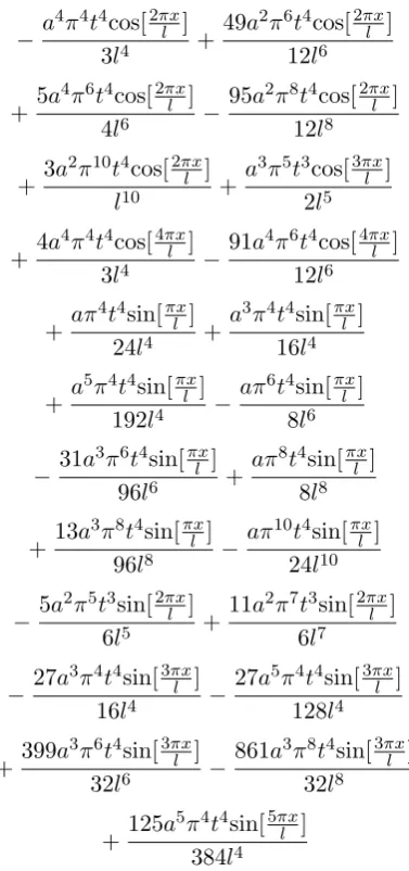
v4 =−
aπ5t3cos[πxl ] 6l5 +
aπ7t3cos[πxl ] 3l7
−aπ9t3cos[πxl ]
6l9 −
−a4π4t4cos[2πxl ]
3l4 +
49a2π6t4cos[2πxl ] 12l6
+5a
4π6t4cos[2πx l ]
4l6 −
95a2π8t4cos[2πxl ] 12l8
+3a
2π10t4cos[2πx l ]
l10 +
a3π5t3cos[3πxl ] 2l5
+4a
4π4t4cos[4πx l ]
3l4 −
91a4π6t4cos[4πx l ]
12l6
+aπ
4t4sin[πx l ]
24l4 +
a3π4t4sin[πxl ] 16l4
+a
5π4t4sin[πx l ]
192l4 −
aπ6t4sin[πxl ] 8l6
− 31a3π6t4sin[
πx l ]
96l6 +
aπ8t4sin[πxl ] 8l8
+13a
3π8t4sin[πx l ]
96l8 −
aπ10t4sin[πxl ] 24l10
− 5a2π5t3sin[2πxl ]
6l5 +
11a2π7t3sin[2πxl ] 6l7
−27a3π4t4sin[3πxl ]
16l4 −
27a5π4t4sin[3πxl ] 128l4
+399a
3π6t4sin[3πx l ]
32l6 −
861a3π8t4sin[3πxl ] 32l8
+125a
5π4t4sin[5πx l ]
384l4
and proceeding in the same way for other terms, we obtainv5,v6,v7.... By takingp= 1, in (5.13), we can obtain the solution of given model prob-lem (5), so that u = limp→1v =v0+v1+v2+
v3+....
6
Numerical Experiments
In this Section, we reveal physical behaviors of so-lution profiles for the equations discussed above by solving different cases with different ranges of all the parameters under consideration. In all the cases, we observe that for t > 0 the solu-tion evolves so that all the conservasolu-tion laws are satisfied.
Example 6.1 In case I, the KdV equation u˙t+u˙x+6 u u˙x+ u˙xxx=0, 0 ≤x≤l.
Figure 1: Wave profiles at time 0.1,1 forρ= 1,0.1 respectively.
with the initial condition at t = 0 is given
by u0(x) = ρ2sech2
(√ ρx 2 −7
)
. Solution profiles
Figure 2: Wave profiles at different times t = 0.6,0.8,1 andt= 0.01 respectively.
at time 0.1,1 forρ = 1,0.1 respectively. Here we have monitored sharp peaks achieving maximum height 0.005089,0.0002188 atx= 14,43. Surface plots for this case study can be seen in Fig. 2for ρ = 1,0.5 in the time interval −1≤t≤1. If we
look at these plots, it is observed that the con-tinuous solution profile that comes into picture is associated with dispersive wave component of the solution. next wave solution is depicted in Fig. 3
within the range−10≤x≤10 at timest= 0.5,1 and corresponding surface plot is plotted in Fig.
4within the spatial range−10≤x≤10 and time range−0.5≤t≤0.5,−1≤t≤1 respectively. In case II, we have KdV equation (6.1), for the initial stateu0(x) =−n(n+ 1)sec2x, which results inn solitons that propagate with different velocities. Particularly for n= 2, we have u0(x) =−6sec2x for which results are shown through figs. 5 achiev-ing different depth levels. At negative times, the deeper soliton, which moves faster, approaches the shallower one. At t = 0 they combine to give u0(x) = −6sec2x, which is a single trough of depth 6 and, after the encounter, the deeper soliton has overtaken the shallower one and both resume their original shape and speed. However, as a result of the interaction, the shallower soli-ton experiences a delay and the deeper solisoli-ton is speeded up. The wave profile plotted at different times t= 0.6,0.8,1 andt= 0.01 is shown in Fig.
5. In Fig. 6, the solution profile depicts two waves where the taller one catches the shorter coalesces to form a single wave. The interaction seems vis-ible at the very first sight. A careful examination of the wave profiles shows that the taller one has moved forward and the shorter goes backward.
Example 6.2 In the second example, we con-sider numerical experiments made for the prob-lem (4).
In the first case we have the given initial condi-tion u0 = 0.8
√
sech[kx]. In Fig. 7, simulation is carried out at different times t = 0,0.5,1,1.5,2 by taking a = 2, b = 1, k = 1, c = 4 in the range
−15 ≤ x ≤ 20 which produces each soliton of amplitude 1.215 moving to the left.
In the next case, for the initial condition
u(x,0) =
(
12c A′+B′
)1/2 ,
where
Figure 3: Wave profiles plotted at different times t= 0.6,0.8,1 andt= 0.01.
B′ =αsinh[2√c/bx]
corresponding analytical solution is
u(x, t) =
(
12c A+B
)1/2
Figure 4: Surface plots within the time range−0.5≤ t≤0.5,−1≤t≤1 respectively.
where
A=a(1 +√1 +α2cosh[2√c/b(x−ct)],
Figure 5: Wave profiles plotted at different times t= 0.6,0.8,1 andt= 0.01.
In 2D case, results are produced by taking a = 24, b= 1, α= 0.1 within the range−15≤x≤20 with c = 2, at times 0.1,0.5,1 and 0,0.8,1.5 re-spectively. Here, we observe soliton amplitude to be 0.7137 and 0.4986 for 2D plots (xranging from
Figure 6: Wave profiles plotted att= 0.05 andt= 0.1 .
Figure 7: Solution u(x, t) at different times t = 0,0.5,1,1.5,2 withc= 4,3 respectively.
solution is obtained for this case is
u(x, t) =
(
12c A1 +B1
)1/2 .
Figure 8: Solution u(x, t) at different times t = 0.1,0.5,1 andt= 0,0.8,1.5 withc= 2,1 respectively for 2D plots and surface plot within the time range t∈[0,1].
where
Figure 9: Solution u(x, t) at different times t = 0,0.5,1 withc= 2,1 respectively for 2D plots and sur-face plot within the time ranget∈[0,1] andt∈[−7,7] respectively.
B1=ıαsinh[2√−c/b(x−ct)]A perspective view of the solution for this case is given in Fig. 9we ob-serve the periodic solution profiles and emerge on
Figure 10: Wave profiles att= 0,15,30 and surface plot for the time range 0≤t≤50.
respec-Figure 11: Wave profiles at t = 2 and surface plot for the time range 0≤t≤2.
tively. It leads to wave amplitudes 0.5035 and 0.7062. Snapshots of the function profile in the form of surface can also be seen with c= 2, with x ∈ [−6,6], t ∈ [0,1] and x ∈ [−4,4], t ∈ [−7,7] respectively.
Example 6.3 This time we deal with RLW equa-tion. With the boundary conditions u → 0
as x → ±∞, and initial condition u(x,0) = 3csech2(k(x−x0)), this solution corresponds to
the motion of a single solitary wave with ampli-tude 3c and width k, initially centered at x0 is presented trough figs.
In the first simulation, a wave profile is ob-served at different times t = 0,15,30. At the very beginning, near x = 0, sharp edge at t = 0 is observed and later as the wave front moves on, its position is changed with the passage of time from x = 20,40 and corre-sponding surface plot is shown in Fig. 10. In the next case, we study the interaction of two solitary waves. As initial condition, we have u(x,0) = 3c1sech2(k1(x−x1)) + 3c2sech2(k2(x−
x2)) where k1 = 1/2
√
εc1/µ(1 +εc1), and k2 = 1/2√εc2/µ(1 +εc2). Here, the one of the ampli-tude is 3c1sited atx=x1and amplitude 3c2sited atx=x2. An interaction occurs when the larger is placed to the left of the smaller. We study such an interaction with k1 =k2 = 0.5, x1 = 15, x2 = 35, c1 = 1.0, c2 = 0.5 running the simulation us-ing the range 0 ≤ x ≤ 40 which can be seen in Fig. 11.
7
Conclusion
In this work, we have used the homotopy per-turbation method (HPM) for standard KDV and RLW equations. The HPM has the capabilities to bereave the complicated differential equation models to number of simple iterative models once the effective initial guess satisfying the boundary conditions is made and leads to generic solutions in addition to their rapid convergence. The algorithm developed facilitates for less time consuming. Also even for smaller values desirable solutions are obtained. The results are comparable to analytic ones. The HPM has been observed to be powerful tool with its addition advantages and suitability for computer simula-tions over the existing tools having potential to be used in more complicated partial differential equation systems.
References
[1] S. Dhawan, S. Kapoor, S. Kumar, S. Rawat,
Contemporary review of techniques for the so-lution of nonlinear Burgers equation, Journal of Computational Science, J. Comput. Science 3 (2012) 405-419.
[2] D.J. Korteweg , G. de Vries,On the change of form of long waves advancing in a rectangular canal and on a new type of long stationary waves, Phil. Mag. J. Science 39 (1895) 422-443.
[4] A. C. Vliegenthart, On finite difference method for Korteweg-de Vries equation, J. Eng. Math. 5 (1971) 137-155.
[5] S. V. Vladimirov, M. Y. Yu, V. N. Tsytovich,
Recent advances in the theory of nonlinear surface waves, Physics Reports 241 (1994) 1-63.
[6] D. H. Peregrine, Calculations of the develop-ment of an undular bore, J. Fluid Mech 25 (1966) 321-330.
[7] D. H. Peregrine, Long waves on a beach, J. Fluid Mech 27 (1967) 815-827.
[8] R. K. Dodd, J. C. Eilbeck, J. D. Gibbon, H. C. Morris, Solitons and nonlinear wave equa-tions, New York: Academic Press (1982).
[9] Siraj-ul-Islam, A. J. Khattak, Ikram A. Tir-mizi, A meshfree method for numerical solu-tion of KdV equasolu-tion, Engineering Analysis with Boundary Elements 32 (2008) 849-855.
[10] A. A. Soliman, M. H. Hussien, Collocation solution for RLW equation with septic spline, Applied Mathematics and Computation 161 (2005) 623-636.
[11] J. H. He, Homotopy perturbation technique, Comp. Meth. Appl. Mech. Engng 178 (1999) 257-262.
[12] J. H. He,The homotopy perturbation method for nonlinear oscillators with discontinuities, Appl. Math. Comput 151 (2004) 287-292.
[13] Sh. S. Behzadia, A.Yildirim,A method to es-timate the solution of a weakly singular non-linear integro-differential equations by ap-plying the Homotopy methods, International Journal of Industrial Mathematics 4 (2012) 41-51.
[14] E. Babolian, A. R. Vahidi, Z. Azimzadeh,
An improvement to the homotopy perturba-tion method for solving integro-differential equations, International Journal of Industrial Mathematics 4 (2012) 353-363.
[15] J. H. He, A note on the homotopy perturba-tion method, Thermal Science 14 (2010) 565-568.
[16] D. Grover, Virendra Kumar and Dinkar Sharma, A Comparitive Study Of Numeri-cal Techniques And Homotopy Perturbation Method For Solving Parabolic Equation And Non-Linear Equations, International Journal for Computational Methods in Engineering Science & Mechanics (Accepted).
[17] S. J. Liao, The proposed homotopy analysis technique for the solution of nonlinear prob-lems, PhD thesis, Shanghai Jiao Tong Uni-versity, 1992.
[18] S. J. Liao, Beyond Perturbation: Intro-duction to the Homotopy Analysis Method, Chapman and Hall/CRC Press, Boca Raton, (2003).
[19] S. J. Liao, Notes on the homotopy analysis method, some definitions and theorems, Com-mun. in Nonlinear Sci. and Numer. Simulat 14 (2009) 983-997.
[20] S. J. Liao, Topology and geometry for physi-cists, Academic Press, Florida Press (1983).
[21] S. Abbasbandy, Homotopy analysis method for heat radiation equations, International Communications in Heat and Mass Transfer 34 (2007) 380-387.
[22] S. Abbasbandy, Y. Tan, S. J. Liao, Newton-homotopy analysis method for nonlinear equa-tions, Applied Mathematics and Computa-tion 188 (2007) 1794-1800.
[23] M. Sajid, T. Hayat, S. Asghar, On the an-alytic solution of the steady flow of a fourth grade fluid, Phy. Lett. A 355 (2006).
[25] Sushila Rathore, Devendra Kumar, Jagdev Singh, Sumit Gupta, Homotopy Analysis Sumudu Transform Method for Nonlinear Equations, International Journal of Industrial Mathematics 4 (2012) 301-314.
[26] S. Abbasbandy,The application of homotopy analysis method to nonlinear equations aris-ing in heat transfer, Physics Letters A 360 (2006) 109-113.
S. Dhawan received Ph.D in Math-ematics from National Institute of Technology Jalandhar India, in 2012, Post-doctoral fellow, Na-tional Board for Higher Mathemat-ics, Department of Atomic Energy, Govt. of India. She is currently working as Assistant Professor in Mathematics at D.A.V. University Jalandhar, India. Her re-search interests are heat transfer, fluid dynamics, FEM, Wavelets and related areas.
D. Grover is working as Assitant Professor at Graphic Era Univer-sity Dehradun, India. He has been working in several research fields on computational , numerical anal-ysis techniques. He is member of various National/International sci-entific bodies. He has (co)authored many re-search papers in the Journals of high interna-tional repute.
S. Kumar is Professor, Department of Mathematics, Dr. B. R. Ambed-kar National Institute of Technol-ogy, Jalandhar, India. He re-ceived M.Sc. degree in Mathemat-ics in 1973, from Indian Institute of Technology, Kanpur, India and Ph.D. degree in 1981, from Indian Institute of Technology, Delhi, India. His research interests are Numerical Analysis: Finite element methods,