VOLUME 39, ARTICLE 35, PAGES 927
,
962
PUBLISHED 25 OCTOBER 2018
https://www.demographic-research.org/Volumes/Vol39/35/ DOI: 10.4054/DemRes.2018.39.35
Research Article
Fertility responses to individual and contextual
unemployment: Differences by socioeconomic
background
Wei-hsin Yu
Shengwei Sun
© 2018 Wei-hsin Yu & Shengwei Sun.
This open-access work is published under the terms of the Creative Commons Attribution 3.0 Germany (CC BY 3.0 DE), which permits use, reproduction, and distribution in any medium, provided the original author(s) and source are given credit.
1 Introduction 928
2 Research on unemployment and childbearing 930
3 Heterogeneous effects of unemployment on fertility 933
4 Data and variables 936
5 Analytic strategy 941
6 Results 943
7 Discussion and conclusions 953
8 Acknowledgements 956
Fertility responses to individual and contextual unemployment:
Differences by socioeconomic background
Wei-hsin Yu1
Shengwei Sun2
Abstract
BACKGROUND
Although research on the consequences of economic recession has long linked unemployment with childbearing, it rarely distinguishes the effects of individuals’ own unemployment and their surroundings’ unemployment levels on their likelihood of having children. Even fewer studies compare how these effects vary for different groups of individuals.
OBJECTIVE
In this study we specifically ask whether fertility timings in the United States are more sensitive to the unemployment rates of individuals’ immediate surroundings or to their own unemployment. Moreover, we investigate whether young adults with different educational levels and parental resources may adjust their childbearing timing differently in response to their own employment status and local unemployment rates.
METHODS
Using 17 rounds of data from the National Longitudinal Survey of Youth 1997, we fit discrete-time event history models predicting men’s and women’s pace of childbearing.
RESULTS
The analysis indicates that relatively disadvantaged young adults, such as those with low education or parents with low education, tend to delay childbirth in response to high local unemployment rates but are less likely than the more advantaged to defer childbearing when facing their own unemployment.
CONCLUSIONS
We argue that the disadvantaged are relatively sensitive to the local unemployment rate but relatively insensitive to their own unemployment compared to those with fewer disadvantages, because the former suffer more from unemployment in times of
economic turmoil, while having lower prospects of economic improvement once having become unemployed.
CONTRIBUTION
Results from this study elucidate how rising unemployment rates shape fertility patterns and indicate the need to consider the effect of parental socioeconomic status on men’s childbearing transitions. Furthermore, our findings help reconcile the debate on how well disadvantaged women’s childbearing timing corresponds to their varying economic conditions.
1. Introduction
Research on life course transitions has long emphasized the impact of economic prospects on the decision to bear children (Becker 1960; Easterlin 1973). Because drastic changes in macroeconomic conditions, such as economic recession, likely alter individuals’ economic prospects, they may further affect fertility rates (Sobotka, Skirbekk, and Philipov 2011). Although much prior research has tested the theory that individuals’ pursuit of parenthood corresponds to macroeconomic shifts (Sobotka, Skirbekk, and Philipov 2011), the recent experience of the Great Recession and its slow recovery has led researchers to pay increasing attention to how changing economic environments are responsible for alterations in childbearing patterns in the United States and elsewhere (Kreyenfeld, Andersson, and Pailhé 2012; Morgan, Cumberworth, and Wimer 2011; Schneider 2017; Schneider and Hastings 2015).
more individuals suffering from job loss, and how much it results from increased anxiety due to the fear of losing jobs among those who have not been unemployed.
Aside from rarely distinguishing fertility responses to individual unemployment from responses to contextual unemployment, prior research has not examined whether different groups of people respond in the same way to changes in their own employment status and in their labor markets’ unemployment rates. Because economic recessions often lead to more job losses for workers with less education (Hoynes, Miller, and Schaller 2012; Sobotka, Skirbekk, and Philipov 2011), those among the employed with less education or fewer other resources may be more sensitive to increasing unemployment in their local economies. However, experiencing unemployment differs from witnessing rising unemployment rates in that in the former situation people with different skill levels are not subject to a different likelihood of losing their job – they are all jobless already. Therefore, if different people have different tendencies to postpone parenthood based upon their own unemployment, it should have to do with their varying prospects of recovering from unemployment rather than their risk of unemployment. Because unemployment is more harmful to and more enduring for those with less skills and resources (Gangl 2004), once unemployed such people may expect less economic improvement in the near future and thus see less benefit in postponing childbearing. As some researchers suggest, women with generally low income potential may delink their fertility decisions from their economic condition because full financial security seems unattainable anyway (Edin and Kefalas 2005; Gibson-Davis 2009).
family socioeconomic status, a factor that has long been shown to shape long-term occupational attainment (Blau and Duncan 1967; Laurison and Friedman 2016; Sewell, Haller, and Portes 1969) but is generally overlooked in research on economic prospects and childbearing. By analyzing different people’s responses to their own unemployment and to their local economy’s unemployment rates, we shed light on the ways in which increases in unemployment during economic downturns may contribute to changes in fertility.
2. Research on unemployment and childbearing
Classic economic theories of fertility have long provided the foundation for understanding the effect of unemployment on childbearing (Sobotka, Skirbekk, and Philipov 2011). Likening children to durable goods, Becker (1960) argues that couples’ demand for children is conditioned by the extent to which they can afford them. Because the cost of childrearing spans many years, couples may consider not only a certain level of financial resources but also economic stability to be prerequisites for parenthood. Concerned about the affordability of children, couples are also likely to postpone or forgo parenthood when the cost of childrearing increases in relation to their long-term income. One way in which the relative cost of having a child rises is through individuals’ unemployment. As prior research has shown, a period of unemployment subjects individuals to a considerable, if not complete, loss of income, a heightened sense of anxiety over their economic future, and decreased earnings even after they land jobs (DiPrete 2002; DiPrete and McManus 2000; Gangl 2004). These changes are likely to raise the relative cost, or the perceived relative cost, of childbearing. Consequently, unemployed people may be less likely to transition to parenthood.
An alternative perspective concerning unemployment and childbearing focuses on the opportunity cost of childbearing, rather than the relative cost to income (Butz and Ward 1979; Inanc 2015; Schmitt 2012; Sobotka, Skirbekk, and Philipov 2011). Because motherhood tends to decrease women’s time and energy for paid work, resulting in their lower earnings (Budig and England 2001), in contexts where most women spend a considerable part of their life being employed, childbearing almost always comes with an opportunity cost for women. This cost varies by women’s job status and economic prospects. For example, once a woman becomes unemployed she no longer faces the possibility of losing earnings through childbearing. Her opportunity cost of having a child hence reduces to zero (as far as earnings are concerned). Because a low opportunity cost constitutes an incentive to have a child, the experience of unemployment may accelerate women’s transition to motherhood. By the same token, women are likely to perceive greater chances of job and income losses when unemployment rates rise in their local economies, even if they do not actually become unemployed. At the very least, as local unemployment grows, women are likely to see fewer promising job opportunities and expect less earnings growth. Either way, higher contextual unemployment can be expected to decrease women’s perceived opportunity cost of childbearing, thereby raising fertility.
Given the inconsistency in fertility responses to individual and contextual unemployment in existing research, we propose a third perspective, derived from prospect theory, and contend that individuals ultimately evaluate the uncertainty related to the risk of unemployment differently from how they evaluate the uncertainty after becoming unemployed. Prospect theory, originating in social psychology and advocated by behavioral economists, posits that individuals are not always rational when evaluating their risk of gain and loss (Kahneman and Tversky 1979). As individuals’ perception of wellbeing declines more with financial losses than it increases with gains (Kahneman 2003), they tend to be more wary of losses than appreciative of gains. The greater sensitivity to potential losses affects individuals’ decision-making. Most people, for example, prefer not to gamble when they have equal chances of winning and losing, even if the amount they could win is moderately higher than the amount they could lose (Mullainathan and Thaler 2000). Also central to prospect theory is the claim that the way in which individuals evaluate risk depends on their current status quo or point of reference. Because individuals’ perception of potential gains and losses are relative to their reference point, their preferences may change with alterations in reference points (Tversky and Kahneman 1991).
Following the arguments about the sensitivity to losses and the importance of a reference point, individuals may be very concerned about their economic status when their local unemployment rate rises, as they perceive potential losses in relation to the status quo. By contrast, for those who have already been unemployed the loss has been realized and the uncertainty pertains only to when they will gain earnings. Because individuals may give more weight to uncertainty about losses than uncertainty about gains, job holders encountering heightened unemployment rates in their surroundings might be more likely than the unemployed to see their economic conditions as too dire to afford children, despite the reality that the former’s future income is higher. This scenario may be especially likely for the relatively disadvantaged in the labor market, as they face much greater uncertainty with rising unemployment rates. At the minimum, being unemployed alters individuals’ current state – that is, their reference point. This change is likely to make the considerations of unemployed people regarding decision-making different from those of people merely facing unemployment risk. Whereas the former’s preference for having a child soon may depend on their calculation of the chance of economic improvement, the latter’s may be based on their assessment of the risk of economic loss.
the unemployment rate in their local labor market.3 We therefore have limited
information on whether local unemployment is still relevant to individuals’ fertility timing after taking into account their own employment status, or how individuals’ unemployment is linked to their childbearing, net of the unemployment rate in their immediate surroundings. Moreover, most existing research linking aggregate-level unemployment to fertility uses unemployment rates of geographic units that are much broader than the local labor markets in which individuals are situated, such as states or countries (Adserà 2005, 2011; Cherlin et al. 2013; Schneider and Hastings 2015).4 As
previous research on the United States shows, even during economic downturns there is wide variation in unemployment chances across different localities within each state, not to mention within the country (Thiede and Monnat 2016). The country- or state-level unemployment rate may also not accurately reflect individuals’ exposure to the risk of unemployment, which is typically through hearing about business closures and layoffs, or knowing people with difficulty finding jobs in their community (Ananat, Gassman-Pines, and Gibson-Davis 2013).
3. Heterogeneous effects of unemployment on fertility
Beyond the question of whether individuals assess the uncertainty linked to their own unemployment and their local unemployment level in similar ways, it is also important to ask whether the associations of individual- and context-level unemployment with fertility behavior are universal for those from different socioeconomic backgrounds. Much research indicates that economic downturns have diverse effects on individuals with different characteristics (Elsby, Hobijn, and Sahin 2010; Hoynes, Miller, and Schaller 2012). For example, during the Great Recession of the late 2000s, less-educated individuals were far more likely to experience job loss and unemployment (Hout, Levanon, and Cumberworth 2011). The differential likelihood by education suggests that people with divergent educational levels may also perceive unemployment risk during recessions differently. That is to say, individuals with more schooling may perceive less increase in the cost of having a child in relation to their income, or less
3 To our knowledge, Kravdal’s (2002) analysis of family formation in Norway is the only study that includes
both individuals’ own unemployment and the unemployment rate in their local labor market as predictors. Although two other studies also distinguish aggregate- from individual-level unemployment experiences, one does not actually estimate the effect of aggregate-level unemployment rates (Hofmann, Kreyenfeld, and Uhlendorff 2017) and the other fails to measure the unemployment rate of the local labor market that individuals face (de Lange et al. 2014).
4 Besides Kravdal (2002), Ananat, Gassman-Pines, and Gibson-Davis’s (2013) study is another exception that
substantial decreases in the opportunity cost of childbearing with rises in local unemployment rates. Either way, the differential perception should lead to a weaker association between aggregate-level unemployment rate and fertility timing for more-educated people.
In addition to educational attainment, individuals’ risks of unemployment may also vary by their family background. Although research on the uneven impacts of economic recessions rarely focuses on the consequences for individuals of divergent family backgrounds, sociologists have long demonstrated that those whose parents have higher socioeconomic status fare better in the labor market (Blau and Duncan 1967; Sewell, Haller, and Portes 1969). Because parents with higher socioeconomic status are more able to cultivate their children’s social and cultural capital (Lareau 2011; Lin 1999), their children are likely to have an advantage in the labor market over their equally educated peers (Laurison and Friedman 2016). Such an advantage may help the perceived risks of unemployment for people of higher-class origin in times of recession. Moreover, individuals from higher socioeconomic backgrounds can potentially receive help from their parents to better weather unemployment. Help from parents is especially likely during young adulthood (i.e., in individuals’ 20s and early 30s), a period when many also make decisions about starting a family. Both the potentially lower unemployment risk and potentially greater parental help may make young adults from well-off families less likely to postpone childbearing in response to rising unemployment rates in their surroundings.
Nevertheless, using individual-level survey data, Schneider and Hastings (2015) find evidence that contradicts the claim of a disconnection between childbearing and financial concerns among the disadvantaged: Unmarried women with high school or less education had lower fertility rates in states with higher unemployment rates during the years of the Great Recession. Despite this finding, their study focuses mainly on whether unmarried disadvantaged women’s family responses change with macroeconomic shifts, rather than how the association between unemployment and fertility varies for different groups within the general population. In addition, Schneider and Hastings’s study does not use the unemployment rate of individuals’ local economy, nor does it make a distinction between individual and contextual unemployment.
Interestingly, when using actual alterations in income and earnings in a period other than the Great Recession, Gibson-Davis (2009) finds that individual-level changes are irrelevant to low-income couples’ childbearing decisions. A study using data from Denmark and Germany further shows that less-educated women barely change their fertility behavior during their periods of unemployment (Kreyenfeld and Andersson 2014). Taken together, these findings raise yet another possibility: Fertility responses of the relatively disadvantaged to their own unemployment, an individual-level economic change, may differ from their responses to increases in contextual unemployment. As our earlier discussion of behavioral economists’ accounts suggests, because high local unemployment implies greater risk of financial losses, disadvantaged women may be more sensitive to rising local unemployment rates than their own unemployment. Moreover, following the model of reference dependence, if unemployed people’s childbearing decisions are based on when and how much they can improve their current financial state, then the low expectation of future economic gains for the disadvantaged will also dampen their perceived benefit of postponing childbearing until recovering from unemployment. As a result, disadvantaged women’s fertility timings may be less responsive to their own unemployment than their more advantaged counterparts’.
4. Data and variables
The data for this study come from Rounds 1–17 of the National Longitudinal Survey of Youth 1997 (NLSY97), which contains a nationally representative sample of individuals born between 1980 and 1984. Beginning in 1997, the NLSY97 has interviewed respondents annually through 2011/12 (Round 15) and biannually ever since. At Round 17, fielded in 2015/16, the NLSY97 respondents were 30 to 36 years of age, with 74% of the women and 61% of the men interviewed having at least one child.5 Our data therefore enables us to capture a contemporary cohort’s childbearing
experiences throughout the period of early adulthood, during which individuals are especially vulnerable to the risk of economic downturn and unemployment (Bell and Blanchflower 2011). Although some prior research on economic security and fertility only focuses on women’s experiences (Edin and Kefalas 2005; Schneider and Hastings 2015), we include both men and women in our sample, as several studies show that men and women have different fertility responses to the experience of unemployment (Kravdal 2002; Kreyenfeld and Andersson 2014; Pailhé and Solaz 2012). Women, for example, may be more likely to see their spell of unemployment as a window with a low opportunity cost of childbearing, while men may be more inclined to postpone childbearing when experiencing unemployment, given their socially prescribed role as their family’s provider.
To conduct an event history analysis of the transitions to childbirth (which we elaborate later), we combine all the rounds to create person-year data, with time-varying information for each respondent. Given our focus on how individuals’ unemployment status is linked to their childbearing transitions, we exclude periods when the experience of unemployment is unlikely to be meaningful to one’s economic wellbeing, such as early and middle adolescence. We therefore eliminate person-years before respondents turned 18 years old from the sample.6 Because the event of childbirth is
lagged in our analysis – that is, we use respondents’ information at a given time point to predict the subsequent occurrence of childbirth – and we have no way of telling whether respondents had a child after the last round in which they appeared in the NLSY97, the sample also excludes the person-year observations from that round in the analysis.7 For
5 Even though the NLSY97 data does not allow us to observe the entire period of childbearing years for
women, we should note that the vast majority of women who would ever experience childbearing had already had one or more births by Round 17, as 15% to 20% of US women typically remain childless throughout their childbearing years (Livingston 2015).
6 This selection, however, does not mean that we assume the risk of entering parenthood starts at age 18. We
discuss how we use conditional likelihood models to handle the left-truncation issue in a later part of the section.
7 Information from the last round of respondents appearing in the NLSY97, however, was used to construct
the statistical analysis we use all person-year observations when respondents were exposed to the risk of making the decision to have a child 9 months later – 40,511 person-years for men and 40,630 person-years for women.8
Given that our objective is to study how changes in contextual and individual unemployment are relevant to the timing of childbearing, the dependent variable for our event history analysis is the occurrence of a childbirth. We code this variable as 1 if a biological child was born between 9 and 18 months from the time respondents were interviewed. The NLSY97 asked both male and female respondents to report births of all biological children regardless of whether the children lived with them. We only consider births that occurred after 9 months because it generally takes 9 months for a child to be born; any child born within 9 months is unlikely based on considerations of respondents’ economic and other conditions at interview time.9 We use 18 months as
the upper bound, to avoid allowing enough time for two consecutive births. In an exploratory analysis, however, we found that using childbirths that occurred within a different time period, such as from the next 9 to 21 months, does not alter the results in a meaningful way. We include all childbirths that occurred during the observed period, rather than just first childbirth, so that we do not need to exclude all those who entered parenthood before turning 18 years of age. Besides, it is reasonable to expect economic prospects to affect more than just the first birth. Individuals may very well postpone having a second or third child if they do not feel economically secure enough to afford the expenses related to rearing another child. An additional analysis, not shown here, nevertheless yielded similar results when we restricted the outcomes to first childbirth.10
To investigate how respondents’ childbearing transitions correspond to their own and others’ unemployment experiences, we introduce time-varying variables of respondents’ employment status and local unemployment rates into the models. We measure employment status in three categories – employed, unemployed, and out of the labor force – based on respondents’ reports at the time of interview. We follow NLSY97’s definition of unemployment, which is a state during which a person is jobless and spends time on looking for a job; other jobless periods are coded as out of
8 Specifically, we assume that respondents were at risk of making a decision to have a child 9 or more months
later if they or their partners were not already pregnant with a child at the interview time. The data therefore excludes the person-years where respondents were less than 9 months to a childbirth from the time of the interview. Because men may have other partners while expecting a child, we also conducted an additional analysis without such a restriction for men. The results were not substantively different.
9 Lagging the dependent variable, a childbirth, by 9 months also enables us to avoid the possibility of reverse
causality – namely, a person becoming unemployed as a result of pregnancy or childbearing, due to employers’ discrimination against pregnant women or his or her reduced effort at work following a childbirth. 10 Separate models for births other than the first one are likely to encounter the problem of sample selectivity,
the labor force. Distinguishing unemployment from out of the labor force is important, especially for women, because women who expect to leave the labor force for motherhood may quit their jobs as they try to conceive, but they are unlikely to actively look for jobs during this period. The distinction based on job search activities therefore helps us rule out the scenario that women choose to be jobless in anticipation of motherhood. The local unemployment rate is derived from the geocode data provided by the Bureau of Labor Statistics (BLS) for the NLSY97 respondents during each
interview year.11 Specifically, the BLS provides the unemployment rate for
respondents’ metropolitan statistical area or core-based statistical area,12 either of which
generally captures the local labor market. Compared to most previous studies that rely on state- or nation-level unemployment rates (e.g., Adserà 2005; Cherlin et al. 2013; Hofmann, Kreyenfeld, and Uhlendorff 2017; Schneider and Hastings 2015), our use of the unemployment rates of respondents’ local economies can more precisely measure the extent of unemployment to which they could be exposed, thus more accurately reflecting their perceived risks of unemployment.
To examine how people with different educational levels and family backgrounds may differ in their fertility responses to their own and others’ unemployment, we further include respondents’ and their parents’ years of completed education.13 We use
parents’ years of education as a proxy for family socioeconomic status because educational attainment is known to be highly related to earnings and occupational status (Blau and Duncan 1967; Sewell, Haller, and Portes 1969), and it is more reliable in providing the long-term prospects of parental economic standing than parental income or occupation taken at an arbitrary time point (e.g., at the beginning of a longitudinal survey, as in the case of the NLSY97). We measure parental education with the parent’s years of education reported at Round 1 of the NLSY97, using the higher of the two if responses for both parents are available. We also include a binary indicator for being enrolled in school at the time of interview.
11 Because a recent study indicates that fertility declines may precede rises in local unemployment rates
(Buckles, Hungerman, and Lugauer 2018), we also fitted additional models in which we used the unemployment rate of the year following the interview year or even the year after that, instead of the unemployment rate of the interview year. Such lagged unemployment rates would allow us to capture unobserved macroeconomic shifts prior to increases in local unemployment that may affect fertility decisions. We, however, did not find the lagged unemployment rates to yield any significant associations with childbearing.
12 If a respondent did not live in a metropolitan statistical area or core-based statistical area, the BLS reported
the unemployment rate of the proportion of the state that is not incorporated into any metropolitan statistical area for his or her local unemployment rate. About 9% of the person-year observations in the analytic sample were not in metropolitan or core-based statistical areas.
13 In an exploratory analysis we measured both respondents’ and their parents’ education based on the degrees
In addition to respondents’ and their parents’ education, the models incorporate several variables related to respondents’ economic prospects and fertility decisions. To begin we include respondents’ race or ethnicity, measured in four categories based on the NLSY97’s classification: (1) non-Hispanic white, (2) non-Hispanic black, (3) Hispanic, and (4) other. Next, we introduce respondents’ annual income, adjusted for inflation to 2012 dollars and measured in $1,000 units, as well as their cumulative work experience since age 14 (in months). Because respondents were asked to report their total income during the year preceding the interview, those who were currently unemployed could still have income. Controlling for personal income in the models enables us to tell whether the status of unemployment, beyond directly altering individuals’ current earnings, is still relevant to individuals’ fertility decisions. We also include an indicator of whether respondents lived with a parent at the time of interview, as this living arrangement might lower the economic impact of unemployment. Because the family structure in which individuals grew up is likely to affect their considerations about starting a family (McLanahan and Bumpass 1988) we further include respondents’ family structures at 12 years old, divided into four groups: (1) families with two biological parents, (2) single-mother families, (3) step-parent families, and (4) other conditions.
The statistical models include time-varying controls for respondents’ geographic location. We use a binary indicator for living in an urban area and a categorical variable for the region in which respondents were located (Northeast, North Central, South, or West, as defined by the Census Bureau).14 Other than their current location, we also
consider the fact that individuals may move to a new location as a result of a job offer, or that they may enter unemployment because of a major move. In either case, the move, rather than unemployment at the individual or contextual level, may be more relevant to individuals’ pace of childbearing. Thus, we further create a time-varying variable indicating that respondents migrated to their county recently (i.e., between the previous and current rounds of the survey).
Moreover, we control for respondents’ union status, measured in the following categories: (1) never-married and not cohabiting; (2) never-married and cohabiting; (3) married; and (4) divorced, separated, and widowed. We further include the number of childbirths that respondents had experienced by each observed time.15 Because the
relationship between the number of existing children and the transition to childbearing may not be linear we measure number of children in categories: (1) zero, (2) one, (3)
14 When there is no information on whether respondents lived in urban areas, we consider their living area to
be urban if they lived in what the Census Bureau defines as a metropolitan statistical area.
15 Throughout the rest of the paper we refer to this variable as the number of children for simplicity, even
two, (4) three or more. Based on our exploratory analysis, further dividing the three-or-more category or using a linear measure of the number of children made little difference to the main results. Given that individuals’ age may also affect their decision to have a child, we control for whether respondents were in one of the following age categories at the time of interview: (1) 18–22, (2) 23–29, and (3) 30–36. Using alternative age categories, as we did in an exploratory analysis, hardly altered the main results.
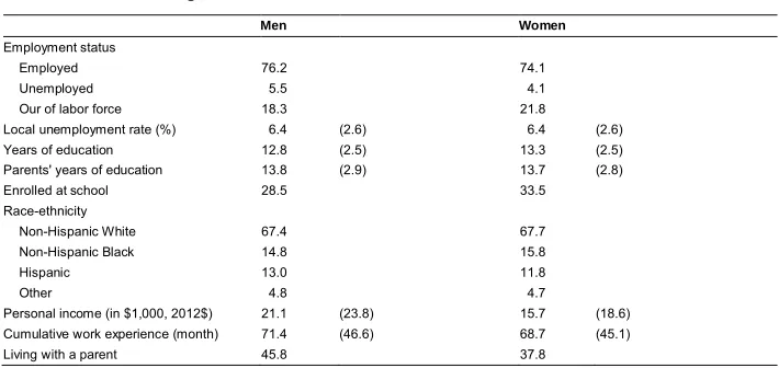
Table 1 presents descriptive statistics from the analytical sample. The proportions and means presented in the table are based on person-year observations, rather than individuals. Thus, although unemployment as a state captures only 5.5% of the person-year sample for men and 4.1% of the person-person-year sample for women, the proportion of the NLSY97 respondents who have ever been unemployed is much higher. Specifically, 47.5% of respondents in the analytic sample reported being unemployed at one or more of the interviews since they had turned 18 years old. The actual prevalence of unemployment experience is even greater, as this percentage does not include those who had undergone an unemployment spell between interviews. In addition to the fact that a good proportion of the NLSY97 respondents had experienced unemployment, these respondents’ local unemployment rates also varied fairly widely during the observed period, with most of the observations falling between 2% (1st percentile) and
15% (99th percentile) and the average being around 6%. Overall, the sample provides
considerable variation, allowing us to examine how differences in individual and contextual employment are relevant to childbearing transitions.
Table 1: Descriptive statistics
Men Women
Employment status
Employed 76.2 74.1
Unemployed 5.5 4.1
Our of labor force 18.3 21.8
Local unemployment rate (%) 6.4 (2.6) 6.4 (2.6) Years of education 12.8 (2.5) 13.3 (2.5) Parents' years of education 13.8 (2.9) 13.7 (2.8) Enrolled at school 28.5 33.5
Race-ethnicity
Non-Hispanic White 67.4 67.7 Non-Hispanic Black 14.8 15.8
Hispanic 13.0 11.8
Other 4.8 4.7
Table 1: (Continued)
Men Women
Family structure at age 12
Two biological parents 53.5 50.0 Single mother 31.4 33.7
Step-parent 5.7 7.8
Others 9.4 8.5
Urban area 77.5 77.3
Region
Northeast 17.7 16.7
North central 26.2 25.0
South 34.7 36.8
West 21.4 21.6
Moved since last round 8.3 8.4 Marital status
Never married, not cohabiting 67.3 54.9 Never married, cohabiting 12.7 15.7
Married 16.9 24.6
Separated/divorced/widowed 3.2 4.8 Number of existing children
None 74.3 62.0
One 14.3 17.7
Two 7.3 12.7
Three or more 4.1 7.6 Age
18–22 40.7 40.2
23–29 49.9 50.1
30~ 9.4 9.7
N of person-year observations 40,511 40,630 N of respondents 4,215 4,023
Note: The descriptive statistics are based on the analytic sample for the transitions to childbearing, the unit for which is person-year. The numbers are calculated with the NLSY97 longitudinal weights that adjust both for the initial sample design and attrition over time. All the numbers followed by parentheses are means, with their respective standard deviation presented in the parentheses, whereas the rest of the numbers are in percent.
5. Analytic strategy
We adopt an event history approach to examine men’s and women’s pace of childbearing, focusing on the different reactions of those with varying education and parental education to individual and contextual unemployment. Specifically, we use discrete-time hazard models (Yamaguchi 1991), which can be expressed as follows:
ln[pit/(1 −pit)] = γ0+ ∑αjDurjit+ γ1Empit + γ2UEit + γ3Eduit + γ4PEduit
+ γ5Empit×Eduit + γ6Empit×PEduit + γ7UEit×Eduit
wherepitis the probability of having a childbirth soon for theith respondent at timet, conditional on this event not occurring earlier; γ0 is the intercept; ∑αj denotes the
coefficients forjdummy variables measuring the duration of exposure; γ1indicates the
effect of respondents’ own employment status, including unemployment, on the hazard rate of childbirth; γ2is the effect of the local unemployment rate (UEit); γ3and γ4are the
coefficients for respondents’ and their parents’ years of education, respectively; γ5is the
coefficient for the interaction between respondents’ employment status and their
education; γ6 denotes the coefficient for the interaction between respondents’
employment status and their parents’ education; γ7 and γ8 are the effects for the local
unemployment rate’s interactions with respondents’ and their parents’ education; and Xkit and ∑βk representk controls and their coefficients, respectively.
Our analytical sample begins when respondents turned 18 years old, although in theory respondents’ first exposure to the risk of having a child could be earlier. For this reason, we further utilize the conditional likelihood approach proposed by Guang Guo (1993) to handle left-truncated data. This approach requires us to measure the duration of exposure from when respondents were first exposed to the risk of the event occurring rather than from the time they entered the sample, but the models are otherwise identical to standard discrete-time hazard models. We measure the duration of exposure to the risk of childbearing as the number of months since respondents turned 16 years old if respondents had never had a child before that age, and as the number of months since the occurrence of the last childbirth if respondents had ever had a child. We use age 16 as the beginning of the risk period for childbirth, because few people in our sample experienced a birth before that age.16 A separate analysis, not presented here,
indicated that making a different assumption, such as assuming that the risk period starts at age 18, did not affect our main results. Based on our exploration of how the chances of childbearing change with time, we construct 5 dummies to capture the duration period: (1) 1–24 months, (2) 25–48 months, (3) 49–72 months, (4) 73–120 months, and (5) 120 months and more.
Because discrete-time hazard rate models ultimately rely on logistic regression techniques, they are similar to logistic models in the potential to suffer from estimation bias when the models employ interaction terms (Mood 2010). To ensure that the results are not sensitive to our modeling choice, we also fit linear probability models with the same variables as in the discrete-time hazard models for an additional check. Furthermore, although our models include an extensive set of individual-level attributes that may affect childbearing, it remains possible that contextual factors other than the local unemployment rate can potentially account for the effect of this rate. Likewise,
16 For those whose first childbirth occurred before they turned 16 years old, we treat the month after the
other unobserved events occurring during a given year, such as shifts in inflation or mortgage rates, may correlate with local unemployment rate and at the same time affect individuals’ economic outlook, thereby altering individuals’ likelihood of experiencing a birth. Given these possibilities, we also fit additional linear probability models with fixed effects for both the county in which respondents resided and the survey round from which they were observed.17 The inclusion of these fixed effects enables us to take
into account all unmeasured time-invariant characteristics of respondents’ counties and the calendar year. Because the NLSY97 oversampled certain minority groups and inevitably has attrition across waves, we apply longitudinal sampling weights and estimate robust errors for all models.18 In addition, we estimate separate models for men
and women, as factors shaping the two groups’ fertility decisions often differ (e.g., Schmitt 2012).
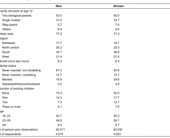
6. Results
Table 2 shows results from a set of discrete-time hazard rate models predicting the occurrence of a childbirth. The models specifically assess whether employment status and local unemployment rate are universally associated with transition to childbearing, and whether the associations are consistent with the predictions from the perspective emphasizing the relative cost of having a child to individuals’ income or the one highlighting the opportunity cost of childbearing. Because individuals’ unemployment status tends to be related to the unemployment rate in their local labor market, we first estimate the two separately. We then include both in the third model for each gender group to estimate the effect of each net of the other. Regardless of the model specifications, however, neither individual nor contextual unemployment is significantly associated with a subsequent childbirth. The nonsignificant results also hold for both men and women. Because previous research has found for Germany that the negative effect of individuals’ unemployment is larger when national unemployment rates are relatively high (Hofmann, Kreyenfeld, and Uhlendorff 2017),
17 In additional analysis we further fitted unconditional fixed-effects logit models with county and year fixed
effects. We did not find meaningful changes in the main results. Unconditional fixed-effects logit models, however, require us to eliminate observations from the same county or year if their outcomes do not vary, not to mention that such models are subject to a higher risk of estimation bias (Katz 2001). We therefore opted for presenting the linear fixed-effects models in the paper.
18 Because childbirth is a repeatable event, some respondents would have experienced multiple childbirth
we also tested an additional model, not presented here, with an interaction between respondents’ employment status and their local unemployment. The interaction between respondents’ unemployment status and their local unemployment rate was not statistically significant either. Thus, regardless of their local economic conditions, unemployed men and women, on average, do not postpone childbearing more than those with jobs.
Table 2: Discrete-time hazard rate models predicting childbearing transitions by gender
Men Women
Model 1 Model 2 Model 3 Model 4 Model 5 Model 6
Employment status (ref. employed):
Unemployed –0.004 0.003 –0.014 –0.014 (0.098) (0.098) (0.102) (0.102) OLF –0.127† –0.121† 0.052 0.053
(0.073) (0.073) (0.055) (0.055) Local unemployment rate –0.011 –0.010 –0.001 –0.001
(0.010) (0.010) (0.009) (0.009) Education –0.009 –0.007 –0.009 0.005 0.004 0.005
(0.012) (0.012) (0.012) (0.011) (0.011) (0.011) Parental education –0.028** –0.029** –0.028** –0.033*** –0.033*** –0.033***
(0.009) (0.009) (0.009) (0.008) (0.008) (0.008) School enrollment –0.478*** –0.495*** –0.480*** –0.541*** –0.537*** –0.541***
(0.074) (0.073) (0.074) (0.060) (0.060) (0.060) Race-ethnicity (ref. white)
Non-Hispanic black 0.550*** 0.548*** 0.552*** 0.419*** 0.416*** 0.419*** (0.062) (0.062) (0.062) (0.054) (0.054) (0.054) Hispanic 0.199** 0.203** 0.201** 0.094 0.093 0.094
(0.068) (0.068) (0.068) (0.061) (0.061) (0.061) Other races –0.406* –0.410* –0.409* –0.179 –0.178 –0.179
(0.161) (0.161) (0.161) (0.128) (0.128) (0.128) Personal income 0.003* 0.003** 0.003* 0.003* 0.003* 0.003* (0.001) (0.001) (0.001) (0.001) (0.001) (0.001) Cumulative work experience –0.002* –0.002* –0.002* –0.001† –0.002* –0.001† (0.001) (0.001) (0.001) (0.001) (0.001) (0.001) Living with parent(s) –0.123* –0.119* –0.121* –0.124* –0.123* –0.124* (0.060) (0.060) (0.060) (0.054) (0.054) (0.054) Family structure, age 12 (ref.two biological parents):
Single-mother –0.004 –0.004 –0.004 0.121* 0.121* 0.121* (0.054) (0.054) (0.054) (0.049) (0.049) (0.049) Step-parent 0.032 0.032 0.031 0.188* 0.188* 0.188* (0.099) (0.099) (0.100) (0.078) (0.078) (0.078) Others 0.010 0.009 0.011 –0.015 –0.015 –0.015
(0.077) (0.077) (0.077) (0.073) (0.073) (0.073) Urban area 0.004 0.002 0.001 –0.025 –0.026 –0.026
(0.059) (0.058) (0.058) (0.052) (0.052) (0.052) Region (ref. northeast)
North Central 0.254*** 0.261*** 0.260*** 0.149* 0.150* 0.149* (0.075) (0.076) (0.076) (0.070) (0.070) (0.070) South 0.033 0.033 0.031 0.103 0.103 0.103
(0.073) (0.073) (0.073) (0.065) (0.065) (0.065) West 0.106 0.116 0.116 0.060 0.062 0.061
Table 2: (Continued)
Men Women
Model 1 Model 2 Model 3 Model 1 Model 2 Model 3
Moved since last round 0.134 0.126 0.132 –0.239** –0.235** –0.239** (0.086) (0.086) (0.086) (0.085) (0.085) (0.085) Marital status (ref.never married, not cohabiting)
Never married, cohabiting 0.930*** 0.940*** 0.931*** 0.573*** 0.574*** 0.573*** (0.076) (0.075) (0.076) (0.065) (0.065) (0.065) Married 1.650*** 1.659*** 1.652*** 1.162*** 1.166*** 1.162***
(0.075) (0.075) (0.075) (0.062) (0.062) (0.062) Separated, divorced, widowed 0.822*** 0.827*** 0.825*** 0.803*** 0.805*** 0.803***
(0.137) (0.137) (0.137) (0.103) (0.103) (0.103) Number of children (ref. none)
One 0.292** 0.295*** 0.301*** 0.411*** 0.416*** 0.412*** (0.089) (0.089) (0.089) (0.072) (0.072) (0.072) Two –0.241* –0.241* –0.231* –0.178† –0.171† –0.176† (0.115) (0.115) (0.115) (0.092) (0.092) (0.093) Three or more –0.092 –0.091 –0.080 –0.429*** –0.420*** –0.427***
(0.129) (0.129) (0.130) (0.110) (0.111) (0.111) Age (ref.18–22)
23–29 –0.232** –0.229** –0.220** –0.324*** –0.315*** –0.323*** (0.081) (0.082) (0.082) (0.070) (0.070) (0.070) 30~ –0.378** –0.400** –0.374** –0.513*** –0.494*** –0.512***
(0.126) (0.125) (0.126) (0.114) (0.113) (0.114) Duration of exposure (ref. 0–24 months)
25–48 –0.181* –0.181* –0.179* –0.116† –0.120† –0.116† (0.075) (0.075) (0.075) (0.062) (0.062) (0.062) 49–72 –0.291*** –0.288*** –0.286*** –0.428*** –0.432*** –0.427***
(0.084) (0.084) (0.084) (0.073) (0.073) (0.073) 72–120 –0.358*** –0.358*** –0.358*** –0.544*** –0.550*** –0.544***
(0.089) (0.089) (0.090) (0.082) (0.082) (0.082) 120+ –0.345** –0.337** –0.328** –0.348*** –0.345*** –0.346***
(0.116) (0.117) (0.117) (0.102) (0.103) (0.103) Constant –2.486*** –2.486*** –2.443*** –2.132*** –2.104*** –2.126***
(0.214) (0.215) (0.218) (0.194) (0.195) (0.196) N of person-year observations 40,511 40,511 40,511 40,630 40,630 40,630 Note: The NLSY97’s longitudinal weights are applied for model estimations. Numbers in parentheses are robust standard errors. †p < 0.1; *p < 0.05; **p < 0.01; ***p < 0.001
Although the results for individual and contextual unemployment are nonsignificant in Table 2, the results for the other variables are largely consistent with what one typically would expect, enhancing our confidence in the models. Men and women with higher personal income experience childbearing at a faster rate.19 African
American men and women have greater odds of experiencing a childbirth than their Hispanic white counterparts. Hispanic men also have greater odds than non-Hispanic white men. Unsurprisingly, compared to men who are never married and not
19 Because those who were unemployed may also have had lower income during the past year, we also tried
cohabiting, the odds of having a child are greater for men who are married and cohabiting. The number of existing children also matters somewhat: Individuals with only one child have greater odds of having another one than those with more or fewer children. For women, being from a single-parent family increases the odds of transitioning to childbearing, whereas having recently migrated decreases such odds, suggesting the upheaval from a major move may be a deterrent for motherhood.
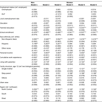
To examine whether the association between unemployment and fertility differs between the more and less disadvantaged groups in the labor market, Tables 3 and 4 present a series of models that include one or more of the following interaction terms: interaction between individuals’ employment status and their education, between their employment status and parental education, between the local unemployment rate and own education, and between the local unemployment rate and parental education. We build models with differing complexity to ensure that the results are not sensitive to model specifications.20 Specifically, we include one of the interaction terms in each of
the first four discrete-time hazard rate models. Next, we present a model with all four interaction terms (Model 5). We then remove all interactions that do not generate significant results to produce the optimal model (Model 6). To test whether the results from the optimal model are robust without the use of logistic regression techniques, we also include the same predictors in a linear probability model (Model 7). Finally, we add county and year fixed effects in Model 8 to further verify the robustness of the results.
The discrete-time model results for men, presented in Table 3, show significant coefficients for the local unemployment rate and its interactions with education and parental education. For men who themselves and whose parents have relatively few years of education the local unemployment rate is negatively associated with the odds of having a childbirth soon, but this association weakens with increases in both men’s and their parents’ education. By contrast, the interaction between men’s own unemployment and their education yields no significant coefficient. Nevertheless, the interaction between their unemployment status and parental education is significant. Specifically, Model 6 shows a positive main effect for unemployment, along with a negative coefficient for its interaction with parental education. Model 7 further indicates that the interaction results remain similar to those in discrete-time hazard rate models, in the sense that both their signs and relative strengths vis-à-vis the main effects are consistent, even if we do not use logistic regression techniques. Adding county and year fixed effects, as in Model 8, also does not change the results in a meaningful way.
20 For the same reason, we also tried models that excluded parental education and all the interactions with
Table 3: Regression results for men’s transitions to childbearing
Discrete-time hazard rate models Linear probability
models Model 1 Model 2 Model 3 Model 4 Model 5 Model 6 Model 7 Model 8
Education 0.004 –0.011 –0.103*** –0.011 –0.072* –0.082** –0.004* –0.005** (0.013) (0.012) (0.028) (0.012) (0.030) (0.029) (0.002) (0.002) Parental education –0.029** –0.013 –0.028** –0.101*** –0.063** –0.059* –0.003** –0.003* (0.009) (0.010) (0.009) (0.023) (0.024) (0.024) (0.001) (0.001) Employment status (ref. employed):
Unemployed 0.823 1.029* 0.007 0.001 1.386* 1.049* 0.050* 0.052* (0.547) (0.435) (0.098) (0.098) (0.649) (0.437) (0.025) (0.025) Out of labor force 0.918* 0.947*** –0.118 –0.116 1.329*** 0.919*** 0.016 0.017
(0.370) (0.264) (0.073) (0.073) (0.389) (0.265) (0.013) (0.013) Unemployed × education –0.071 –0.041
(0.048) (0.048) Out of labor force × education –0.090** –0.053
(0.032) (0.034)
Unemployed × parental education –0.082* –0.072* –0.083* –0.004* –0.004* (0.035) (0.035) (0.035) (0.002) (0.002) Out of labor force × parental education –0.082*** –0.065** –0.080*** –0.002† –0.002† (0.020) (0.022) (0.020) (0.001) (0.001) Local unemployment rate –0.011 –0.011 –0.182*** –0.151*** –0.224*** –0.228*** –0.012*** –0.011***
(0.010) (0.010) (0.047) (0.042) (0.052) (0.052) (0.003) (0.003) Local unemployment rate × education 0.013*** 0.010* 0.010** 0.001* 0.001**
(0.004) (0.004) (0.004) (0.000) (0.000) Local unemployment rate × parental education 0.011*** 0.007* 0.007* 0.0004* 0.0004*
(0.003) (0.003) (0.003) (0.000) (0.000) Socioeconomic controls Included Included Included Included Included Included Included Included County fixed effects Included
Year fixed effects Included
N 40,511 40,511 40,511 40,511 40,511 40,511 40,511 40,511 Note: The NLSY97’s longitudinal weights are applied for model estimations. Numbers in parentheses are robust standard errors. The socioeconomic characteristics controlled in the models are the same as those in the models in Table 2, including school enrolment status, race-ethnicity, personal income, cumulative work experience, whether to live with a parent, family structure at age 12, being in urban area, region, marital status, number of existing children, and age. The models also include duration of exposure to the risk of transitioning to childbearing, of which the coefficients, along with the coefficients for the constant, are omitted from the table to conserve space.
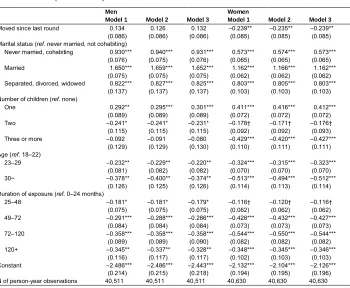
Table 4: Regression results for women’s transitions to childbearing
Discrete-time hazard rate models Linear probability
models Model 1 Model 2 Model 3 Model 4 Model 5 Model 6 Model 7 Model 8
Education 0.016 0.005 –0.086*** 0.004 –0.068** –0.074** –0.005* –0.005** (0.012) (0.011) (0.024) (0.011) (0.026) (0.025) (0.002) (0.002) Parental education –0.033*** –0.027** –0.032*** –0.078*** –0.052** –0.032*** –0.002*** –0.002***
(0.008) (0.009) (0.008) (0.018) (0.019) (0.008) (0.001) (0.001) Employment status (ref. employed):
Unemployed 0.927† –0.174 –0.013 –0.011 0.603 0.922† 0.062† 0.063† (0.481) (0.441) (0.103) (0.102) (0.589) (0.473) (0.034) (0.034) OLF 0.474† 0.399† 0.053 0.053 0.595* 0.435 0.039† 0.043* (0.275) (0.209) (0.055) (0.055) (0.298) (0.272) (0.021) (0.021) Unemployed × education –0.078* –0.086* –0.077* –0.005* –0.005* (0.039) (0.039) (0.039) (0.003) (0.003) OLF × education –0.034 –0.022 –0.031 –0.003† –0.003† (0.022) (0.023) (0.022) (0.002) (0.002) Unemployed × parental education 0.013 0.033
(0.034) (0.037) OLF × parental education –0.027† –0.020
(0.016) (0.017)
Local unemployment rate –0.001 –0.001 –0.174*** –0.090** –0.200*** –0.171*** –0.013*** –0.012*** (0.009) (0.009) (0.042) (0.033) (0.045) (0.042) (0.003) (0.003) Local unemployment rate × education 0.013*** 0.012*** 0.013*** 0.001*** 0.001***
(0.003) (0.003) (0.003) (0.000) (0.000) Local unemployment rate × parental education 0.007** 0.003
(0.002) (0.002)
Socioeconomic controls Included Included Included Included Included Included Included Included County fixed effects Included
Year fixed effects Included
N of person-year observations 40,630 40,630 40,630 40,630 40,630 40,630 40,630 40,630
Note: The NLSY97’s longitudinal weights are applied for model estimations. Numbers in parentheses are robust standard errors. The socioeconomic characteristics controlled in the models are the same as those in the models in Table 2, including school enrolment status, race-ethnicity, personal income, cumulative work experience, whether to live with a parent, family structure at age 12, being in urban area, region, marital status, number of existing children, and age. The models also include duration of exposure to the risk of transitioning to childbearing, of which the coefficients, along with the coefficients for the constant, are omitted from the table to conserve space.
†p < 0.1; *p < 0.05; **p < 0.01; ***p < 0.001.
calculate all the probabilities assuming that the other predictors are identical to the sample means – that is, we assume the hypothetical men are otherwise ‘average.’ For Panels A and B, which show the probabilities by local unemployment rate, we also assume the hypothetical men to be employed, as this is the mode for employment status.21
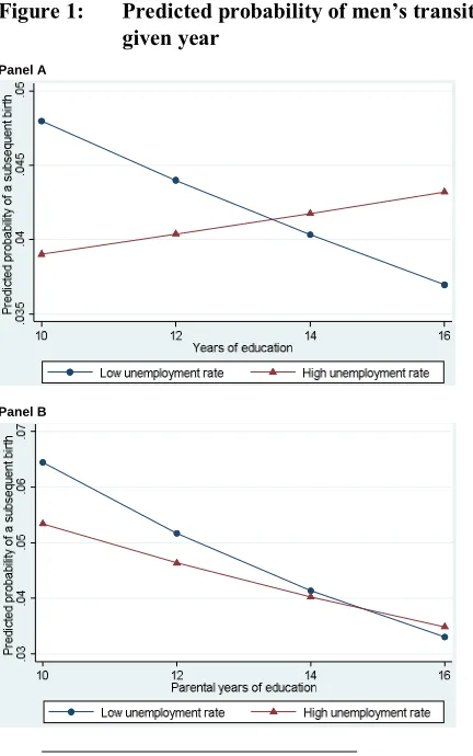
Figure 1: Predicted probability of men’s transition to a childbirth in a given year
Panel A
Panel B
21 In addition to providing a better understanding of the results, using predicted probabilities to represent
Figure 1: (Continued)
Panel C
Note: “High unemployment rate” refers to a local unemployment rate at 10.0%, whereas “low unemployment rate” refers to a 3.7% local unemployment rate. The predicted probabilities are calculated using coefficients from Model 6 in Table 3, with the assumption that all other variables are equal to sample means. Panels A and B also assume that the hypothetical men have jobs.
Panel A in Figure 1 shows that for men with high school or less education (i.e., 12 or 10 years of education), the probability of having a subsequent childbirth is much greater when the local unemployment rate is low rather than high. As men’s years of education increase, however, the predicted probability of transitioning to parenthood while facing high local unemployment increases. Thus, a high contextual unemployment rate delays less-educated men’s childbearing transitions far more than it does those of more-educated men. Regarding how men’s fertility responses to individual and contextual unemployment vary by parental education, Panel B similarly demonstrates that men whose parents have relatively low education – high school or less – have a higher probability of having a child when the local unemployment rate is low as opposed to high. This result, along with the finding that less-educated men are more likely to postpone childbearing in high-unemployment contexts, is consistent with the argument that more disadvantaged workers are more sensitive to rising unemployment rates in their immediate surroundings because they are more likely to suffer from such economic shifts.
unemployment, however, declines sharply with increases in parental education. For men whose parents have some tertiary education (14 and 16 years), having a job is associated with a higher probability of transitioning to childbearing than being unemployed.
Turning to the models for women, results in Table 4 show that the fertility responses to individuals’ own unemployment and their surroundings’ unemployment rates also differ between different groups of women. Specifically, the discrete-time hazard rate models show significant effects for the interactions between education and both individuals’ unemployment and their local unemployment rates. The signs for these interaction terms, however, are in opposite directions. Whereas the association between being unemployed and the transition to a childbirth moves from positive to negative with increases in women’s own education, the association between the local unemployment rate and the transition turns from negative to positive with the same increases. Unlike for men, the interaction term between local unemployment rates and parental education is nonsignificant for women once we also include the interaction terms with education in the model (Model 5). We also find no significant effect for the interaction between parental education and women’s own unemployment status. Thus, women’s fertility responses to individual and contextual unemployment depend on their own education but not their parents’ education. Models 7 and 8 in Table 4 generally replicate the results in Model 6, indicating that the findings from discrete-time hazard rate models are highly reliable.
years). This difference suggests that less-educated women are more sensitive to shifts in local unemployment than highly educated women.
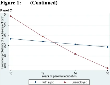
Figure 2: Predicted probability of women’s transition to a childbirth in a given year
Panel A
Panel B
Panel B in Figure 2 indicates that an unemployed woman with less than high school education has a slightly higher probability of having a child soon than her counterpart with a job. The relationship between women’s employment status and predicted probabilities of childbearing, however, changes with years of education. The probability that an unemployed woman will have a child soon decreases considerably with her education, whereas the probability for a woman who has a job and is otherwise identical is fairly constant across years of schooling. As a result, when all other individual attributes and the local unemployment rate are set to be average, women with tertiary education (14 and 16 years) have a much higher probability of transitioning to childbearing when holding a job, as compared to being unemployed. Having a job also alters the childbearing probability much more for women with some college or more education than for women with high school or less education, suggesting that highly educated women are especially sensitive to their own unemployment status.
7. Discussion and conclusions
Although separate research examining the effects of individual and contextual unemployment on childbearing has suggested that individuals respond to their own unemployment and the prevalence of unemployment around them differently, few existing studies systematically compare these responses. Using life history data from young adults and their local unemployment rates, we find that, contrary to research evidence from various European countries (e.g., Adserà 2005; Comolli 2017; Kravdal 2002), neither individual-level nor aggregate-level unemployment has a universal influence on young men’s and women’s childbearing transitions in the United States. Instead, US young adults’ fertility responses to their own unemployment and their local unemployment rate are highly segmented, with different segments of the population responding to individual-level and aggregate-level unemployment. Specifically, the relatively advantaged, such as men with well-educated parents and women with college education, are more likely to delay childbearing upon becoming unemployed than the relatively disadvantaged. At the same time, the relatively disadvantaged are far more likely than the relatively advantaged to postpone childbearing transitions when facing high local unemployment rates.
refutes the argument about the opportunity cost of motherhood. Because this cost reduces more drastically with unemployment for more educated women, if unemployed women were motivated by the lower opportunity cost of having a child, those with more education should be especially likely to accelerate their childbearing transitions. However, we find the opposite.
Ultimately, results from our analysis suggest that young adults’ assessment of the affordability of childbearing is relevant, but their assessment depends on both their actual risk of losing income and their point of reference. To elaborate, less-educated young adults are likely to postpone childrearing when facing high local unemployment rates because their actual likelihood of suffering from rises in unemployment in their surroundings is high. By contrast, this likelihood is low for highly educated young adults, making them unlikely to delay childbirth in response to rising contextual unemployment. At the same time, our finding that less-educated young women do not decelerate their transition to childbearing upon entering unemployment, while their highly educated counterparts do, is consistent with the argument that the unemployed have a different reference point when assessing whether they can currently afford children. For the unemployed, the decision to postpone childbearing depends on the extent to which they expect their economic conditions to improve, rather than on losses already occurred. Because less-educated unemployed women expect less economic improvement from their current state than highly educated unemployed women, the latter are more likely to postpone childbearing transitions.
Interestingly, our result that disadvantaged women delay fertility according to increased local unemployment but not their own experience of unemployment is consistent with the seemingly contradictory findings of Schneider and Hastings (2015) and Gibson-Davis (2009). Whereas Schneider and Hastings find that unmarried women with low socioeconomic status have lower fertility rates in states with higher unemployment rates, Gibson-Davis shows that decreases in individuals’ income do not affect their likelihood of childbearing. Rather than supporting or rejecting the overarching argument that disadvantaged women tend to delink their fertility decisions from economic concerns, our findings, in conjunction with previous evidence, suggest that such women take certain types of economic fluctuation into consideration, but are relatively unaffected by others. As discussed above, disadvantaged women may be very concerned about potential economic losses, but downplay any short-term income reductions that have been realized, including that resulting from unemployment, when considering having a child. By providing a more nuanced understanding of disadvantaged women’s childbearing decisions, our study sheds light on the debate on whether such women delink economic conditions from fertility.
transition to childbearing concentrates on those more likely to suffer from unemployment. The fact that these findings are net of individuals’ own unemployment status indicates that they do not just reflect compositional changes during economic downturns – that is, a larger number of the disadvantaged become unemployed. Rather, among those with jobs the less advantaged are well aware of their greater unemployment risk in a worsening economy, and the advantaged of their minimal risk: their family behaviors reflect the differential risk perceptions.
implications for their total number of children, elucidating how unemployment is linked to fertility behaviors during young adulthood is especially useful for our understanding of how changes in macroeconomic circumstances shape population dynamics. However, future research is needed to ensure the applicability of our findings to a broader population.
8. Acknowledgements
We gratefully acknowledge support from theEunice Kennedy ShriverNational Center
References
Adserà, A. (2005). Vanishing children: From high unemployment to low fertility in
developed countries.American Economic Review 95(2): 189–193.doi:10.1257/
000282805774669763.
Adserà, A. (2011). Where are the babies? Labor market conditions and fertility in
Europe.European Journal of Population 27(1): 1–32.
doi:10.1007/s10680-010-9222-x.
Ahn, N. and Mira, P. (2001). Job bust, baby bust? Evidence from Spain. Journal of
Population Economics 14(3): 505–521.doi:10.1007/s001480100093.
Ananat, E.O., Gassman-Pines, A., and Gibson-Davis, C. (2013). Community-wide job
loss and teenage fertility: Evidence From North Carolina. Demography 50(6):
2151–2171.doi:10.3386/w19003.
Becker, G.S. (1960). An economic analysis of fertility. In: National Bureau of
Economic Research (ed.). Demographic and economic change in developed
countries. New York: Columbia University Press: 209–240.
Bell, D.N.F. and Blanchflower, D.G. (2011). Young people and the Great Recession. Oxford Review of Economic Policy 27(2): 241–267.doi:10.1093/oxrep/grr011.
Blau, P.M. and Duncan, O.D. (1967).The American occupational structure. New York:
John Wiley and Sons.
Buckles, K., Hungerman, D., and Lugauer, S. (2018). Is fertility a leading economic indicator? Cambridge: NBER (National Bureau of Economic Research Working Paper Series 24355).doi:10.3386/w24355.
Budig, M.J. and England, P. (2001). The wage penalty for motherhood. American
Sociological Review 66(2): 204–225.doi:10.2307/2657415.
Butz, W.P. and Ward, M.P. (1979). The emergence of countercyclical US fertility.The American Economic Review 69(3): 318–328.
Cherlin, A., Cumberworth, E., Morgan, S.P., and Wimer, C. (2013). The effects of the
Great Recession on family structure and fertility. The Annals of the American
Comolli, C.L. (2017). The fertility response to the Great Recession in Europe and the United States: Structural economic conditions and perceived economic
uncertainty. Demographic Research 36(51): 1549–1600. doi:10.4054/DemRes.
2017.36.51.
De Lange, M., Wolbers, M.H.J., Gesthuizen, M., and Ultee, W.C. (2014). The impact of macro- and micro-economic uncertainty on family formation in the Netherlands. European Journal of Population 30(2): 161–185. doi:10.1007/s10680-013-9306-5.
DiPrete, T.A. (2002). Life course risks, mobility regimes, and mobility consequences:
A comparison of Sweden, Germany and the United States.American Journal of
Sociology108: 267–309.doi:10.1086/344811.
DiPrete, T.A. and McManus, P.A. (2000). Family change, employment transitions, and the welfare state: Household income dynamics in the United States and
Germany.American Sociological Review 65: 343–370.doi:10.2307/2657461.
Easterlin, R.A. (1973). Relative economic status and the American fertility swing. In:
Sheldon, E.B. (ed.). Family economic behavior: Problems and prospects.
Philadelphia: J.B. Lippincott: 170–227.
Edin, K. (2000). What do low-income single mothers say about marriage? Social
Problems 47(1): 112–133.doi:10.2307/3097154.
Edin, K. and Kefalas, M. (2005). Promises I can keep: Why poor women put
motherhood before marriage: Berkeley: University of California Press.
Edin, K., Kefalas, M.J., and Reed, J.M. (2004). A peek inside the black box: What
marriage means for poor unmarried parents. Journal of Marriage and Family
66(4): 1007–1014.doi:10.1111/j.0022-2445.2004.00072.x.
Elsby, M.W., Hobijn, B., and Sahin, A. (2010). The labor market in the Great Recession. Cambridge: NBER (National Bureau of Economic Research Working Paper Series 15979).doi:10.3386/w15979.
Gangl, M. (2004). Welfare states and the scar effects of unemployment: A comparative
analysis of the United States and West Germany.American Journal ofSociology
109(6): 1319–1364.doi:10.1086/381902.
Gibson-Davis, C.M. (2009). Money, marriage, and children: Testing the financial
expectations and family formation theory. Journal of Marriage and Family
Guo, G. (1993). Event-history analysis for left-truncated data. Sociological Methodology 23: 217–243.doi:10.2307/271011.
Hofmann, B., Kreyenfeld, M., and Uhlendorff, A. (2017). Job displacement and first birth over the business cycle.Demography 54(3): 933–959.doi:10.2307/271011. Hout, M., Levanon, A., and Cumberworth, E. (2011). Job loss and unemployment. In:
Grusky, D.B., Western, B., and Wimer, C. (eds.). The Great Recession. New
York: Russell Sage: 59–81.
Hoynes, H., Miller, D.L., and Schaller, J. (2012). Who suffers during recessions?The Journal of Economic Perspectives 26(3): 27–47.doi:10.1257/jep.26.3.27. Inanc, H. (2015). Unemployment and the timing of parenthood: Implications of
partnership status and partner’s employment. Demographic Research 32(7):
219–250.doi:10.4054/DemRes.2015.32.7.
Kahneman, D. (2003). Maps of bounded rationality: Psychology for behavioral
economics.The American Economic Review 93(5): 1449–1475.doi:10.1257/000
282803322655392.
Kahneman, D. and Tversky, A. (1979). Prospect theory: An analysis of decision under risk.Econometrica 47(2): 263–291.doi:10.2307/1914185.
Katz, E. (2001). Bias in conditional and unconditional fixed effects logit estimation. Political Analysis 9(4): 379–384.doi:10.1093/oxfordjournals.pan.a004876. Kravdal, Ø. (2002). The impact of individual and aggregate unemployment on fertility
in Norway.Demographic Research 6(10): 263–294.doi:10.4054/DemRes.2002.
6.10.
Kreyenfeld, M. and Andersson, G. (2014). Socioeconomic differences in the unemployment and fertility nexus: Evidence from Denmark and Germany. Advances in Life Course Research 21: 59–73.doi:10.1016/j.alcr.2014.01.007
Kreyenfeld, M., Andersson, G., and Pailhé, A. (2012). Economic uncertainty and family
dynamics in Europe: Introduction.Demographic Research Special Collection on
Economic uncertainty and family dynamics in Europe 27(28): 835–852.
doi:10.4054/DemRes.2012.27.28.
Lareau, A. (2011). Unequal childhoods: Class, race, and family life. Berkeley: