Volume 7, 2018, Pages 1–15
PROOFS 2018. 7th International Workshop on Security Proofs for Embedded Systems
Side-Channel Assisted Malware Classifier with Gradient
Descent Correction for Embedded Platforms
Manaar Alam
1, Debdeep Mukhopadhyay
1, Sai Praveen Kadiyala
2, Siew Kei
Lam
2, and Thambipillai Srikanthan
21 Indian Institite of Technology Kharagpur, Kharagpur, West Bengal, India.
[email protected], [email protected]
2
Nanyang Technological University, Singapore.
[email protected], siewkei [email protected], [email protected]
Abstract
Malware detection is still one of the difficult problems in computer security because of the occurrence of newer varieties of malware programs. There has been an enormous effort in developing a generalised solution to this problem, but a little has been done considering the security of resource constraint embedded devices. In this paper, we at-tempt to develop a lightweight malware detection tool designed specifically for embedded platforms using micro-architectural side-channel information obtained through Hardware Performance Counters (HPCs). The methodology aims to develop a distance metric, called
λ, for a given program from a benign set of programs which are expected to execute in the embedded environment. The distance metric is decided based on observations from carefully chosen features, which are tuples of high-level system calls along with low-level HPC events. An idealλ-value for a malicious program is 1, as opposed to 0 for a benign program. However, in reality, the efficacy ofλto classify a malware largely depends on the proper assignment ofweightsto the features. We employ a gradient-descent based learning mechanism to determine optimal choices for these weights. We justify through experimen-tal results on an embedded Linux running on an ARM processor that such a side-channel based learning mechanism improves the classification accuracy significantly compared to an ad-hoc selection of the weights, and leads to significantly low false positives and false negatives in all our test cases.
1
Introduction
model using system calls is presented in [1], which aimed at extracting specific system call pat-terns pertaining to malware and thereby analyzing runtime programs. Owing to the increase in malware feature database, a model, defining bounds for a database, called Bound of Frequency Model (BOFM) is presented in [2]. Many such software protections are bypassed routinely by smart malware writers and are hence inadequate. For instance, the method of observing frequencies of system calls [3] fail to detect kernel-modifying rootkits. On the other hand, modern processors are enabled with dedicated performance monitoring registers, called Hard-ware Performance Counters (HPCs) which provide low-level and sensitive information of events occurring beneath the software stack. These HPC events have been traditionally used as side-channels for compromising ciphers, ranging from RSA [4] to more contemporary Elliptic Curve Cryptography [5]. HPC events have recently been used to detect side-channel attacks [6] and ransomwares [7] in the contemporary systems. However, in this work, we investigate whether these rich side-channels can be utilized to classify malware from benign codes which are typ-ically expected to execute on a target embedded platform. The HPC values are also difficult to manipulate, and thus potentially serve a robust source of information on the system. The usage of HPCs in literature to detect the presence of malware codes have been rather limited, and mostly quite ad-hoc. Early work in malware detection using Hardware Performance Coun-ters (HPCs) was discussed in [8]. Attempts to build a malware detector in hardware using performance counters are done in [9]. Approaches to detect malware that modify the system calls are discussed in [10,11]. In these works, authors focused on counting the hardware events that occur during each system call execution in a guest Virtual Machine thereby identifying the modifications to kernel control flow. However, all of these works either require hardware modification, or employ complex detection architecture which may not be suitable to implement in a resource constraint embedded devices. While few approaches have been based on Machine Learning (ML) [12,13], others have been performing correlation analysis [14,15] to distinguish benign and malware codes. The accuracy of the ML-based methods largely depends on the features chosen; however, the reported works do not stress on the selection of these feature vectors. On the other hand, the later is based on thresholding of the correlation, where the estimation of threshold can be vital, and an ad-hoc decision can lead to a drastic adverse result.
Significance to Embedded Platform
The primary objective of this work is to develop a light-weight malware detection method which targets resource constraint embedded environments. The proposed scheme is ideal for such platforms for the following reasons:
1. Embedded platforms are often aimed at supporting a restricted set of applications. In such a situation, the proposed method is ideally useful, as the reference point for computing the distance metricλis well-defined.
2. The proposed detection scheme is capable of running in a simple embedded Linux without re-quiring any sophisticated libraries.
The scheme is also amenable to an on-line implementation which does not require a large memory to store while evaluation and have a small code size.
Contribution
The technical contributions of the paper are summarized as below:
1. We formalize a concrete side-channel assisted methodology for malware classification on an em-bedded platform. As opposed to existing literature, we attempt to develop a theoretical frame-work by combining statistical tests using side-channel information with learning techniques to arrive at an optimal model for classification.
2. We present a gradient descent based optimization technique to improve the relative sensitivity of the features which comprise of both high-level (common OS utilities), and low-level (HPC) events. This provides significantly better classification accuracy and reduces the false positives and false negatives to a great extent for our test examples.
The overall organization of the paper is as follows: Section 2 presents necessary prelimi-nary background. Section3presents a comprehensive discussion on the proposed methodology with Section4 demonstrating an extensive set of results for an ARM-based embedded system. Finally, Section5concludes our work.
2
Preliminary Background
A fundamental question in several scientific discourses is whether two sets of data are signif-icantly different from each other. A t-test is often used to provide a quantitative value, as a probability, that the meanµof two sets are different. The objective of the test strategy is thus to detect whether there is any deviation from an expected reference distribution.
2.1
Hypothesis testing using
t
-test
Let us consider two samplesX0andX1having mean and standard deviations asµ0,s0andµ1,
s1respectively. A statistical hypothesis callednull hypothesison the equality of two means for
the two samples (denoted as H0: µ0 =µ1) is tested for acceptance or rejection based on the
sample observations. The Welch’s t-test is used for testing the null hypothesis when the two samples have unequal sample variances and unequal sample sizes with the test statistic,
t=rµ0−µ1
s2 0 n0+
s2 1 n1
(1)
where,n0andn1 are the sample sizes ofX0 andX1 respectively. The degree of freedom (ν) is
ν≈
s2 0 n0 +
s2 1 n1
2
s4 0 n2
0ν0+ s4
1 n2
1ν1
where,ν0=n0−1 andν1=n1−1. The null hypothesisH0 is rejected when the test statistic |t|exceeds a threshold defined by the confidence level (α) andν.
2.2
Online Computation of
t
-test
Computation oft-test for large distributions on resource-constrained devices, where expending significant memory for storing these distributions is not possible, can be performed as follows:
Mi,k=Mi,k−1+
xi,k−Mi,k−1
k Si,k=Si,k−1+ xi,k−Mi,k−1
xi,k−Mi,k
wherexi,k, Mi,k,Si,k and ni are kth observation, current mean, sum of squares of differences from the current mean, and sample size respectively for the ith distribution. The sample variance of theith distribution following the calculation iss2
i = Si,k
ni−1. Thet-statistic between the two distributions may now be computed as per Equation (1) as described previously.
2.3
Hardware Performance Counters
Hardware Performance Counters (HPCs) are a set of special purpose registers which are present in most of the modern processor’s Performance Monitoring Unit. These registers can be pro-grammed easily to collect the number of occurrences of different micro-architectural events (like cache misses, branch mispredictions, retired instructions, etc.) during the execution of a pro-gram in the processor. Linuxperfis a widely used tool, for all Linux 2.6.35+ based systems, which can be invoked to access these performance counters with very low granularity. Every popular operating system has HPC-based profilers, but the number and type of performance counter events vary across different Instruction Set Architectures. Most of the modern proces-sors offer thousands of HPC events to monitor, but, only a selected few of them can be observed in parallel because of the restrictions in the number of built-in HPC registers.
3
Overview of the Proposed Methodology
In this section, we first discuss the intuition behind the proposed method. Next, we introduce a formal definition of a distance metric signifying a functional difference from the set of benign programs. Finally, we propose an approach to improve the metric based on error feedback.
3.1
Intuition behind the Approach
The number of malware programs can be unlimited; however, they are expected to perform specific operations like potentially affect the file system, try to hide some files, affect the network, create additional processes, etc. The intuition of our detection strategy is to generate a set of benign operating system library executables, called indicators, which would be monitored in run-time by observing a set of low-level hardware events, called observers. These low-level hardware events can easily be monitored using hardware performance counters (HPCs). We select thoseindicators andobservers, which are most likely to be affected by the malwares.
The types of programs which can execute on a specific Embedded Platform are limited. For example, an iPod is expected to run MP3 and video player programs. We call such programs as benign programs. The idea is based on the hypothesis that the HPC events would vary significantly when a malicious code runs in the system, compared to when a benign program runs on it. So, we try to quantify the functional distance of an unknown program from the set of benign programs defined by some suitable metric. A smaller distance can be interpreted as closeness in functionality to the benign programs, indicating benign nature of the unknown program. Similarly, a larger distance can be interpreted as a significant deviation between functionalities of the unknown program and the set of benign programs, thus indicating a possible malicious nature of the unknown program. Therefore, initial pre-processing would be to create templates of the benign environment, by observing low-level hardware events for the monitored set of indicators. When a potentially unknown malicious code executes, it is expected that the statistics generated by the observers for the indicators are significantly different.
3.2
Formalization of the Distance Metric
Let the set of indicators be denoted as R = {r1, r2,· · · , rp} and the observers as H = {h1, h2,· · · , hq}. The combination of observers and indicators are called tuples. We have a total ofp×q tuples. For any executable,e, when the indicator ri is run in its presence, we observe the hardware performance counterhj using the popular Linuxperf tool. This is per-formed forstrials to minimize the effect of system noise. Let the value of hardware performance counter hj for kth trial when indicator ri is run in presence of e be denoted as αki,j(e). Let θi,j(e) be the distribution ofhj in the presence of bothri ande, containingsobservations, i.e., θi,j(e) ={α1i,j(e), α2i,j(e),· · ·, αsi,j(e)}. When done for allp×qtuples, we obtain a distribution matrix, for the executablee:
D(e) =
θ1,1(e) θ1,2(e) θ1,3(e) . . . θ1,q(e) θ2,1(e) θ2,2(e) θ2,3(e) . . . θ2,q(e)
. . .
. . .
. .
. . .. ... θp,1(e) θp,2(e) θp,3(e) . . . θp,q(e)
Initially we consider a collection of two sets of programs; one which contains malwares and other which contains benign application programs. Let the malware set be denoted as M={m1, m2,· · ·, mk}and the benign application programs asB={b1, b2,· · ·, bl}. After the perf stat collection for both the sets, we obtain two sets of distribution matrices. We denote the distribution matrices for the set of malwares as {D(m1),D(m2),· · · ,D(mk)} and for the set of benign application programs as{D(b1),D(b2),· · ·,D(bl)}.
Algorithm 1:Calculation of Sensitivity Matrix
Data: Sets Containing Benign (B) and Malware (M) Executables, List of Indicator ProgramsR, List of HPC EventsH
Result: Sensitivity MatrixW
forallblinBdo
forallindicators inRdo
Collectperf script results for the events inHwithblin the background;
D(bl) = parsed values for the collected data;
end end
forallmkinMdo
forallindicators inRdo
Collectperf script results for the events inHwithmkin the background;
D(mk) = parsed values for the collected data;
end end
InitializeSensitivity Matrix Wto zero for all (R,H) tuple;
forallri inRdo
forallhjinHdo
forallblinBdo
forallmkinMdo
Calculatet-statistic forD(bl) andD(mk) corresponding to tupleriandhj using
Equation (1);
ift-statistic> tcriticalthen
IncrementW(ri, hj) by 1;
end end end end end
Normalize and returnW;
A basic strategy to assign weights to the tuples is through the count of correct classification of a malware by that tuple. If a tuple (ri, hj) correctly identifies a malware, mx, against a benign program,by, then we increase its count. Since we havep×q tuples, we obtain a count matrix withprows and qcolumns. The values of each cell in the count matrix ranges between 0 and total number of benign and malware program combination, i.e., between [0, k×l]. These counts are then normalized to obtain thesensitivity matrix created based on these tuples. An illustration ofsensitivity matrix (W) is shown below.
W=
w1,1 w1,2 w1,3 . . . w1,q w2,1 w2,2 w2,3 . . . w2,q
. . .
. . .
. .
. . .. ... wp,1 wp,2 wp,3 . . . wp,q
Here,wi,jsignifies a relative importance of indicatorriand observerhjto detect a malware program. Calculation of sensitivity matrix is described in details with the help of Algorithm1. The quantification of the distance metric for an unknown programT from the set of benign samples are shown as follows. We collect the perf stat data forT and obtain the distribution matrixD(T), as described previously. Now this distribution is compared against all thelbenign programs using Welch’s t-test for all the p×q tuples. This univariate analysis constructs a
C=
c1,1 c1,2 c1,3 . . . c1,q c2,1 c2,2 c2,3 . . . c2,q
. . . . . . . . . . .. ... cp,1 cp,2 cp,3 . . . cp,q
MultiplyingCwith the sensitivity matrixW, obtained previously, we get aScore Matrix,S. The score matrix is obtained by element-wise multiplication ofC andW. Thus,S=C W.
Hence,sij=cijwij fori∈ {1,· · ·, p} andj∈ {1,· · ·, q}. We define λas the sum of all the elements in the matrixS. Thus,
λ= p X i=1 q X j=1
si,j= p X i=1 q X j=1
ci,jwi,j (2)
This λ, ranging between 0 and 1, can be interpreted as the quantification of functional distance of the programT from the benign setB because:
• IfT is a benign program, distributions of most of its tuples will be similar to that of the programs in setB. As a result, elements of the count matrixC, i.e.,ci,j, will take lower values. Since, the calculation ofλin Equation (2) depends onci,j and constantwi,j,λwill take lower value.
• Similarly, ifT is a malware program, the distributions of most of its tuples will be different from the programs in setB. Hence, elements of the count matrixCwill take higher values than benign programs and the correspondingλwill be higher than the previous case.
We can quantify lower and higher values by defining a threshold. An unknown program having λ value less than a predefined threshold λt, is termed as a benign program, or else a malware program. Threshold λt is determined by applying 3σ rule on the distribution of λ values obtained for benign programs in setB. Suppose mean and standard deviation obtained from the distribution containing values λ1, λ2, . . ., λl are µB and σB respectively, where λi represents theλvalue forithbenign program in set B. Then the thresholdλ
tis defined as:
λt=µB+ 3σB (3)
Hence, for an unknown programT, having distance metricλunknown, we can conclude:
T is
(
Benign, ifλunknown< λt M alware, otherwise
The decision for an unknown program of being a benign or a malware depends on the threshold of λt. Since the threshold is computed using the 3σanalysis, there are chances for some malware programs having λ value less than the threshold and some benign programs havingλvalue greater than the threshold. In other words, because of the threshold, we could incur false positives as well as false negatives. Moreover, the calculation ofλ depends on the sensitivity matrixW, which is computed beforehand based on a set of benign program Band a set of malware programM. SinceWis a constant matrix, we may not get the optimal value of λas we intended ideally (0 for benign and 1 for malware) and could incur some errors in determining the λvalues. Next, we propose a method to update the matrix W based on the errors calculated on the initial set of benign and malware programs by giving feedback in terms of errors incurred. Our objective is to optimize the matrix such that theλ values for benign and malware programs are close to the ideal values of 0 and 1 respectively. In such a way, the decision making will be free from the dependency on any threshold.
3.3
Improving the Metric based on Error Feedback
As of now, we formalized the distance metricλ for an executable which is lower for a benign program and higher for a malware program. We consider our problem as aBinary Classification
for malware). The classification of a sample depends on its Count MatrixC, Sensitivity Matrix Wand the thresholdλt. The count matrix is constant for a particular sample, as it is obtained by deterministic univariatet-test. Instead of playing around with the thresholdλt, we propose an approach following the principles of Least Mean Square Error, to optimize the sensitivity matrixW, which helps to provide λvalues close to 0 for benign and close to 1 for malwares. This updated sensitivity matrix will be more robust to false-positives and false-negatives which may occur because of the selection of threshold.
In the initial phase we consideredlbenign programs{b1, b2,· · · , bl}andkmalware programs {m1, m2,· · · , mk}to create the sensitivity matrix. We assign each sample,r(r= 1 tol+k), a labely(r), such that,y(r)= 0 for benign andy(r)= 1 for malware. We calculate distance metric
λ(r)for each sample using Equation (2). A standard mathematical way to compute error is by summing the squared deviation of the obtained output from the actual label. Thus we define,
E=X
r
y(r)−λ(r)2 (4)
Since, λ(r) depends on the wi,j’s in sensitivity matrix W, intuitively we say that changes in wi,j increases or decreases the error. The main objective is to iteratively adjust thewi,j’s such that the errorE is minimized. If a change in weight increases (decreases) the error, then we want to decrease (increase) that weight. Mathematically, this means that we look at the derivative of the error with respect to the weight, i.e., we look at ∂E
∂wi,j, which represents the change in the error given a unit change in the weight. The weightwi,j is then updated by the termδwi,j=−η∂w∂Ei,j. Changes for each weight should be proportional to the gradient. Hence, ηis the proportionality constant known aslearning rate and the minus sign indicates to adjust the weight in the negative direction of the gradient to minimize error.
The new weightwti,j+1is updated from the old weightwt
i,j using the following equation:
wti,j+1=wi,jt +δwi,j=wi,jt −η ∂E
∂ wi,j (5)
The weight updation process is described as below. We add a factor of 12 to E for making the calculation convenient. Hence,
E= 1 2
X
r
y(r)−λ(r)
2
∂E
∂wi,j
=−X
r
y(r)−λ(r)∂λ
(r)
∂wi,j
=−X
r
y(r)−λ(r)
∂ ∂wi,j X i X j c(i,jr)wi,j
=−X
r
y(r)−λ(r)c(i,jr) Hence,
δwi,j=−η ∂E
∂wi,j
=ηX r
y(r)−λ(r)c(i,jr) The new updated weight forwti,j will be:
wi,jt+1=wti,j+η
X
r
y(r)−λ(r)c(i,jr) (6)
Algorithm 2:Training Step
Data: Sensitivity MatrixW, Set of Labelsy(r), Count MatrixCfor alll+ksamples, Learning Rate
η, Tolerance Levelξ, Maximum Number of Iterationmax iter
Result: Updated Sensitivity MatrixW0
repeat
forr=1 tol+kdo
Calculateλ(r)using the Equation (2);
end
fori=1 topdo forj=1 toqdo
Updatewi,j using the Equation (6);
end end
CalculateEusing Equation (4);
untilEdoes not change byξin10successive iterations ormax iter is reached;
constant value. We quantify the termdesirable number of iterationsby introducing a parameter namedtolerance level (ξ). We perform the weight updation steps for a maximum of max iter times by monitoringE obtained in each iteration and inspect whether it has been reduced by an amountξ. If the error does not improve by ξin, say, successive 10 iterations, we conclude that, the updated weights have reached to the saturated value and will not improve much. We consider the final updated sensitivity matrix for testing unknown programs.
We define the weight updating steps as training step for the binary classifier, which we describe with the help of Algorithm2.
3.4
Analysis of an Unknown Program
We collect the data for an unknown program T and obtain the distribution matrix D(T), as described previously. Now this distribution is compared against all thelbenign programs using
Welch’s t-test for all the p×q tuples. This univariate analysis constructs a Count Matrix
(C) having p rows and q columns. Multiplying C with the updated sensitivity matrix W0,
obtained in the training phase, we get a Score Matrix, S, and accordingly obtain λunknown using Equation (2). We say that:
T is
(
Benign, ifλunknown≈0
M alware, ifλunknown≈1
The procedure to analyze an unknown program of being malware or benign is described with the help of Algorithm 3. In the next section, we evaluate our proposed approach with detailed experimental results and comparison with state-of-the-art.
4
Experimental Results
In this section, we first present a detailed overview of the experimental setup and then analyze the efficiency of the proposed methodology using a comprehensive set of results.
4.1
Experimental Setup
Algorithm 3:Testing Phase
Data: Distributions of all Benign Executables used for trainingD(B), Updated Sensitivity MatrixW0,
List of Indicator ProgramsR, List of HPC EventsH, Executable of the unknown programT
Result: Decision whetherT is Malware or Benign
forallindicators inRdo
Collectperf script results for the events inHwithT in the background;
D(T) = parsed values for the collected data;
end
InitializeCount Matrix Cto zero for all (R,H) tuple
forallri inRdo
forallhjinHdo
forallblinBdo
Calculatet-statistic forD(bl) andD(T) corresponding to featuresriandhjusing
Equation (1);
ift-statistic> tcriticalthen
IncrementC(ri, hj) by 1;
end end end end
NormalizeC;
Calculateλunknownusing Equation (2);
ifλunknown≈0then
ReturnT as Benign;
end
ifλunknown≈1then
ReturnT as Malware;
end
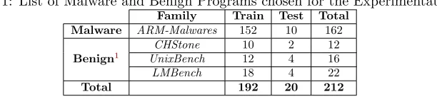
Table 1: List of Malware and Benign Programs chosen for the Experimentation
Family Train Test Total
Malware ARM-Malwares 152 10 162
Benign1
CHStone 10 2 12
UnixBench 12 4 16
LMBench 18 4 22
Total 192 20 212
We collected 162 latest ARM-based malwares from Offensive Computing and VirusShare
database and used 50 standard Linux benchmark programs, such asCHStone,UnixBench, and
LMBench for our analysis. We used these different benchmark programs as a source for the benign reference point. Table 1 shows the separation of all programs into Train and Test
data for offline and online analysis respectively. In this experiment, we consider 5 indica-tors ls, netstat, ps, who, pwd and 6 observers cycles, instructions, cache-references, cache-misses, branches, branch-misses to validate the proposed technique. We collected data for each executable 50 times to minimize the effect of noise.
1The list of some of the benign programs which are quite relevant to the modern day embedded environments
from these benchmark suites are:
1. CHStone: Double-precision floating-point operations (DFADD, DFMUL, DFDIV, etc.), Graphics oper-ations (ADPCM, JPEG, MOTION, etc.), Encryption operoper-ations (AES, BLOWFISH, SHA, etc.).
2. UnixBench: File operations (FSDISK, FSTIME, etc.), Arithmetic operations (SHORT, INT, LONG, etc.), Memory operations (HANOI, DHRY2REG, etc.)
(a) (b)
Figure 1: Distribution of (a)cache-missesand (b)branch-missesfor the indicator program psin presence of AES andMalware.
Table 2: Initial Sensitivity MatrixW for Various Indicator-Observer tuples cycles instructions cache-references cache-misses branches branch-misses ls 0.0274 0.0299 0.0285 0.0208 0.0298 0.0371 ps 0.0513 0.0515 0.0512 0.0375 0.0513 0.0514 who 0.0243 0.0382 0.0366 0.0145 0.0405 0.0184 netstat 0.0264 0.0352 0.0352 0.0171 0.0351 0.0194 pwd 0.0259 0.0414 0.0389 0.0171 0.0392 0.0293
4.2
Validation of Assigning Weights to the Tuples
We present an experiment in this subsection to show the effect of (indicator, observer) tuple in detecting an unknown program as a benign or a malware. We consider a benign programs, namelyAES from CHStone Benchmark Suite, and one malware as mentioned in Table 1, for this experiment. We choose to monitor one indicator program ps and two observers namely cache-misses and branch-misses. The resulting distributions for both the executables are provided in Figure1. The univariatet-statistic for the distributions in Figure1aand Figure1b are−0.4798 and 32.3781 respectively. Thetcritical value for these datasets is 1.6605 with 95% confidence level. Figure1shows clearly that, while the later is able to present a distinguishable distribution, the former is not. It may be noted that the tuple (ps, cache-misses) is not effective for this example but can be effective for other pairs of benign and malware programs. Hence, we do not discard this tuple but rather assign a suitable sensitivity value. This sensitivity list provides a quantification of the goodness of the associations of the indicators with the observers in distinguishing a malware from a set of benign programs.
We followed Algorithm 1 considering the data in Offline phase, as mentioned in Table 1, and obtained an initialsensitivity matrix as shown in Table2.
4.3
Analysis of Unknown Programs using Initial Sensitivity Matrix
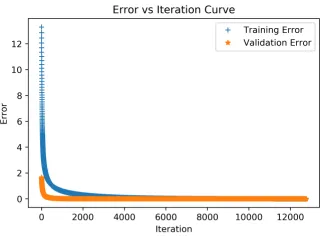
Figure 2: λvalues for 20 Test Programs Figure 3: Errors in each Iteration
Table 3: Updated Sensitivity MatrixW0for Various Indicator-Observer tuples cycles instructions cache-references cache-misses branches branch-misses ls 0.6411 0.8974 1.1656 -0.9028 -0.9583 0.2866 ps 0.6371 -0.0825 -0.5154 0.0533 -0.2367 0.5548 who 0.2735 0.0005 0.1963 -0.4748 -0.0066 -0.1982 netstat -0.3863 -0.2506 -0.0963 0.2996 0.8166 -0.2988 pwd 0.2647 -0.0882 -0.3782 0.3098 0.3533 -1.2136
by assigning some empirical value between [0.62,0.65] instead of 3σanalysis to deal withfalse negativeoccurred in this experiment. But, to find the optimal threshold value which generalizes for all the examples, we need to analyze ample of malware programs with this technique. Still, there will be a chance for some malwares to raise false negatives as well as some benign programs which raise false positives. Hence, we update the sensitivity matrix instead of dealing with the threshold and show the results in the next subsection.
4.4
Updating the Sensitivity Matrix
We update the sensitivity matrix following Algorithm2and usinglearning rate(η) andtolerance level (ξ) to be 10−3 and 10−6 respectively. One major issue with gradient descent algorithm
is that it may overfit2 for the training sample. In order to verify that the proposed gradient
descent model does not overfit for our example, we divided the initial data in online phase into train data and validation data. We update weight based on the new training data and monitor both training and validation error in each iteration. The errors in each iteration is shown in Figure3. Blue line presents errors for training data and Orange line presents errors for validation data. It can be seen that the weight updation does not overfit for our example (as both the errors decrease with increase in iterations) and gradually saturates to optimum3value.
The final sensitivity matrixW0 obtained after weight updation process is shown in Table3.
4.5
Analyzing Unknown Programs on Updated Sensitivity Matrix
The test programs mentioned in Table1are again selected here, like Section4.3, to analyze the efficiency of the proposed method. We followed the approach mentioned in Algorithm 3 and obtained the λunknown values for all the 20 programs, but this time considering the updated sensitivity matrix. The resultingλunknownvalues using both the initial and updated sensitivity
Table 4: Comparison of λ values for the Benign Test Programs using Initial and Updated Sensitivity Matrix
Benign Programs(λunknown)
Initial Sensitivity Matrix 0.5213 0.4979 0.5284 0.5796 0.5718 0.5558 0.5249 0.5636 0.6136 0.4781
Updated Sensitivity Matrix 0 0 0 0 0 0 0 0 0.0589 0
Table 5: Comparison of λ values for the Malware Test Programs using Initial and Updated Sensitivity Matrix
Malware Programs(λunknown)
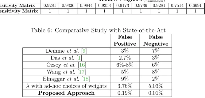
Initial Sensitivity Matrix 0.9281 0.9326 0.9844 0.9353 0.9173 0.9736 0.9281 0.7514 0.6691 0.7465
Updated Sensitivity Matrix 1 1 1 1 1 1 1 1 1 1
Table 6: Comparative Study with State-of-the-Art False
Positive
False Negative Demmeet al.[9] 3% 7%
Daset al.[1] 2.7% 3%
Ozsoyet al.[16] 6%-8% 6%
Wanget al.[17] 5% 8%
Elnaggaret al.[18] 9% 2% λwith ad-hoc choices of weights 3.76% 5.03%
Proposed Approach 0.19% 0.01%
matrices are shown in Table4and Table5. It is clear from both the tables that the separability between benign and malware programs has been increased significantly.
The average separability between benign and malware test programs provided in Table 4 and Table 5, based on the initial sensitivity matrix W is 0.3331 and for updated sensitivity matrixW0 is 0.9941. Hence, for the above dataset we obtain 199.97% increase in separability
between benign and malware programs, which further helps to reduce the confusion in decision making and thereby increases the classification accuracy of the proposed method.
4.6
Comparison of Accuracy with other State-of-the-Art
We evaluated our proposed approach several times by selecting 20 programs randomly during testing as mentioned in Table 1 and compared the result with five other notable approaches mentioned in [9, 1,16,17,18], which also aim to detect and prevent malware executables. We have also presented results of theλ-based classifier based on initial ad-hoc selection of sensitivity matrix to show the effectiveness of weight updation in terms of reducing false positives and false negatives. The comparison is presented in Table6, which clearly shows that the accuracy of the proposed model is best among the recent literature with the given dataset. The table also presents the reduction in false positives and false negatives because of the weight correction. We didn’t consider other notable works in this field to compare with, as they either require hardware modifications or require significant computing resources which do not meet our objective to design a lightweight detection framework.
4.7
Implementation Overhead
resource requirement using the Linux top command for the ARM Cortex-A9 processors and observed that %CPU Usage and %MEM Usage4 are 16.788% and 0.798% respectively. We
observe that the memory usage of the proposed method is almost negligible, though the CPU usage is slightly high, but can be permitted given the performance of the model.
Working of the proposed model depends on the distribution of benign programs, which are collected offline and stored in memory to be used in the online phase. Hence, size of the code and offline dataset are also important considering resource constraint embedded platform. Total virtual memory size used by the model to detect a single program under test is around 9 MB. The value includes the size of all code, data and shared libraries. This low value also establishes the fact that the proposed model is indeed very light-weight in terms of storage requirement.
5
Conclusion
In this paper, we attempt to analyze the side-channel information generated via Hardware Performance Counters (HPCs) and OS calls, to classify malware programs from benign programs which are expected to execute on an embedded processor. We base the classification mechanism on statistical hypothesis, which is a light-weight mechanism and can be easily implemented in low computation devices. The work develops a distance metric, called λ for distinguishing malware programs from benign executions. The work stresses the importance of optimally choosing the weights of the features and proposes a gradient descent based methodology to improve the separability of the malware class from the benign applications. We show through experimentations performed on an embedded Linux on an ARM processor that the combination of the learning technique with side-channel analysis outperforms existing works in reducing false positives and false negatives. We also show that the methodology has very less computational overhead and can be developed in any resource constraint devices running an embedded Linux.
Acknowledgement
We would like to acknowledge Haldia Petrochemicals Ltd. and TCG Foundation for partially supporting the research through the grant entitled “Cyber Security Research in CPS”. We are also grateful to the anonymous reviewers for their insightful comments and suggestions.
References
[1] Sanjeev Das, Yang Liu, Wei Zhang, and Mahintham Chandramohan. Semantics-based online malware detection: towards efficient real-time protection against malware. IEEE transactions on information forensics and security, 11(2):289–302, 2016.
[2] Mahinthan Chandramohan, Hee Beng Kuan Tan, Lionel C Briand, Lwin Khin Shar, and Bindu Madhavi Padmanabhuni. A scalable approach for malware detection through bounded feature space behavior modeling. InAutomated Software Engineering (ASE), 2013 IEEE/ACM 28th International Conference on, pages 312–322. IEEE, 2013.
[3] Federico Maggi, Matteo Matteucci, and Stefano Zanero. Detecting intrusions through system call sequence and argument analysis. IEEE Transactions on Dependable and Secure Computing, 7(4):381–395, 2010.
4The %CPU Usage and %MEM Usage signifies the share of elapsed CPU time and available physical memory
[4] Sarani Bhattacharya and Debdeep Mukhopadhyay. Who watches the watchmen?: Utilizing per-formance monitors for compromising keys of rsa on intel platforms. InInternational Workshop on Cryptographic Hardware and Embedded Systems, pages 248–266. Springer, 2015.
[5] Sarani Bhattacharya and Debdeep Mukhopadhyay. Utilizing performance counters for compro-mising public key ciphers. ACM Transactions on Privacy and Security (TOPS), 21(1):5, 2018. [6] Manaar Alam, Sarani Bhattacharya, Debdeep Mukhopadhyay, and Sourangshu Bhattacharya.
Performance counters to rescue: A machine learning based safeguard against micro-architectural side-channel-attacks. 2017.
[7] Manaar Alam, Sarani Bhattacharya, Debdeep Mukhopadhyay, and Anupam Chattopadhyay. Rap-per: Ransomware prevention via performance counters.arXiv preprint arXiv:1802.03909, 2018. [8] Corey Malone, Mohamed Zahran, and Ramesh Karri. Are hardware performance counters a cost
effective way for integrity checking of programs. In Proceedings of the sixth ACM workshop on Scalable trusted computing, pages 71–76. ACM, 2011.
[9] John Demme, Matthew Maycock, Jared Schmitz, Adrian Tang, Adam Waksman, Simha Sethu-madhavan, and Salvatore Stolfo. On the feasibility of online malware detection with performance counters. InACM SIGARCH Computer Architec. News, volume 41, pages 559–570. ACM, 2013. [10] Xueyang Wang and Ramesh Karri. Numchecker: Detecting kernel control-flow modifying rootkits
by using hardware performance counters. InProceedings of the 50th Annual Design Automation Conference, page 79. ACM, 2013.
[11] Xueyang Wang and Ramesh Karri. Reusing hardware performance counters to detect and identify kernel control-flow modifying rootkits.IEEE Transactions on Computer-Aided Design of Integrated Circuits and Systems, 35(3):485–498, 2016.
[12] Hugo Gascon, Fabian Yamaguchi, Daniel Arp, and Konrad Rieck. Structural detection of android malware using embedded call graphs. In Proceedings of the 2013 ACM workshop on Artificial intelligence and security, pages 45–54. ACM, 2013.
[13] Adrian Tang, Simha Sethumadhavan, and Salvatore J Stolfo. Unsupervised anomaly-based mal-ware detection using hardmal-ware features. InInternational Workshop on Recent Advances in Intru-sion Detection, pages 109–129. Springer, 2014.
[14] Xueyang Wang, Sek Chai, Michael Isnardi, Sehoon Lim, and Ramesh Karri. Hardware performance counter-based malware identification and detection with adaptive compressive sensing. ACM Transactions on Architecture and Code Optimization (TACO), 13(1):3, 2016.
[15] Yanzhi Dou, Kexiong Curtis Zeng, Yaling Yang, and Danfeng Daphne Yao. Madecr: Correlation-based malware detection for cognitive radio. InComputer Communications (INFOCOM), 2015 IEEE Conference on, pages 639–647. IEEE, 2015.
[16] Meltem Ozsoy, Khaled N Khasawneh, Caleb Donovick, Iakov Gorelik, Nael Abu-Ghazaleh, and Dmitry Ponomarev. Hardware-based malware detection using low-level architectural features.
IEEE Transactions on Computers, 65(11):3332–3344, 2016.
[17] Xueyang Wang, Charalambos Konstantinou, Michail Maniatakos, and Ramesh Karri. Confirm: Detecting firmware modifications in embedded systems using hardware performance counters. In
Computer-Aided Design (ICCAD), 2015 IEEE/ACM International Conference on, pages 544–551. IEEE, 2015.