Efficient n-to-n Collision Detection for Space Debris using 4D AABB Trees

Volume 61, 2019, Pages 170–182

ARCH19. 6th International Workshop on Applied Verification of Continuous and Hybrid Systems

Efficient

n

-to-

n

Collision Detection for Space Debris

using 4D AABB Trees

∗

Stanley Bak

and Kerianne Hobbs

1

Safe Sky Analytics Manlius, NY, USA

[email protected]

2

Air Force Research Laboratory, Dayton, OH, USA

[email protected]

Georgia Institute of Technology

[email protected]

Abstract

Collision detection algorithms are used in aerospace, swarm robotics, automotive, video gaming, dynamics simulation and other domains. As many applications of collision detec-tion run online, timing requirements are imposed on the algorithm runtime: algorithms must, at a minimum, keep up with the passage of time. Even offline reachability com-putation can be slowed down by the process of safety checking when n is large and the specification isn-to-n collision avoidance. In practice, this places a limit on the number of objects, n, that can be concurrently tracked or verified. In this paper, we present an improved method for efficient object tracking and collision detection, based on a modified version of the axis-aligned bounding-box (AABB) tree data structure. We consider 4D AABB Trees, where a time dimension is added to the usual three space dimensions, in order to enable per-object time steps when checking for collisions in space-time. We eval-uate the approach on a space debris collision benchmark, demonstrating efficient checking beyond the full catalog of n = 16848 space objects made public by the U.S. Strategic Command onwww.space-track.org.

1

Introduction

The prediction of collisions between large numbers of objects in 3D space is important in many domains such as interactive video games or the verification of cyber-physical systems. In set-based verification methods for dynamical systems, most effort and runtime typically consists of the reachability computation step. However, the process of safety checking can become a bottleneck when the specification is that no objects collide with any other objects (then-to-n

collision detection problem), and the number of objects,n, is large.

∗_{DISTRIBUTION A. Approved for public release; Distribution unlimited. Approval AFRL PA case number}

This was the focus of a recently-proposed benchmark on space debris collision detection [10]. In that work, a method based on axis-aligned bounding box (AABB) trees was proposed and could verify the absence of collisions faster than real-time for around 4000 objects. The key insight there was to perform checking using global variable time steps, versus performing a check at each multiple of a fixed time step. In this work, we modify the approach to also permit variable time steps on a per-object basis. This requires adding a time dimension to the AABB tree data structure, resulting in a method that works on 4D AABB trees. The new result is evaluated on real space debris data made public by the U.S. Strategic Command. In particular, we demonstrate faster-than-real-time tracking is possible with up to about 65000 objects.

Note that in this paper we focus on the discrete-time version of the problem, with a fixed minimum time step, although extensions to continuous time are possible. Further, although applications use collision detection online, we measure the offline performance of the algorithm, and compare the simulated time versus the computation time. Our algorithm is geared towards finding the earliest collision, as this is sufficient for the verification problem and applications may want to react to this event as it may impact future object trajectories. An extended technical report with additional details and a proof of algorithm correctness is available online [1].

2

AABB Trees

Axis-Aligned Bounding Box (AABB) trees [2] are a type of bounding volume hierarchy used in collision detection methods. Bounded volume hierarchies are trees where the leaf nodes represent volumes of individual objects, and inner nodes of the tree correspond to sets that contain every object and set below them in the tree. An AABB tree is a binary tree, where each object and set is represented by an axis-aligned (non-rotated) bounding box. Thus, the root of the tree will be a bounding box that contains every object, and the parent of two leaf nodes will simply be the bounding box containing the two objects. AABB trees can also maintain balance as new objects are inserted and updated using surface area heuristics, so that query operations remain efficient. We do not plan to review all the details of AABB trees here, although detailed introductions are available elsewhere1.

The three operations on AABB trees we will use are:

• insert - AABB trees store a world object and an associated box, usually the object’s occupancy region. Insert operations take such pairs and add them to the AABB tree, possibly performing tree rotations to maintain balance for efficient queries.

• query - Tree queries check if a given box intersects with any previously-inserted box in the tree, returning a list of colliding objects. Queries are performed by starting at the tree root and recursively checking if the query box intersects the left or right child. In the ideal case, half the objects can be discarded at each layer, leading to an efficientO(log(n)) lookup time. This may not be possible if the query box is large or the tree balance is poor.

• update - Objects in an AABB tree can have their bounds updated within an existing tree. This can prevent the need to construct a new tree at every time step.

Tree balancing operations are used to ensureO(log(n)) complexity for each of the operations. Checking allnobjects at a fixed time step therefore takesO(nlog(n)) time. With a time bound

1_{An accessible introduction to AABB trees is available online at www.azurefromthetrenches.com/}

ofT and a time step ofδ, the total runtime for constructing a tree at each step and checking for collisions isO(T_δnlog(n)). In earlier work [10], we improved upon this by considering larger time steps, essentially reducing the T_δ term.

An AABB tree is used for collision detection, and so each object should have an associated 3D bounding box in space, at each point in time. We call this box anoccupancy region. The occupancy region is all points within a cube with faces at a fixed distancerfrom a center point ofpos(t), as defined by the the occupancy region function.

Definition 1 (Occupancy Region). An object’s occupancy region at a fixed time is the set

of 3D space the object takes up at that time. This set is defined by occ(w, t) = {x ∈ _R3 _: kw.pos(t)−xk_∞ ≤ w.r}, where w.pos(t) is the object’s position over time, and w.r is the object’s radius.

3

Collision Detection with 4D AABB Trees

We propose the use of 4D AABB trees for efficiently solving the collision detection problem. Like traditional AABB trees, 4D AABB trees include the usual three space dimensions, but they also have an additional time dimension. Collisions are detected when two objects overlap in both space and time. The 4D nature of the tree allows time to be tracked per-object, so that variable time steps, computed on a per-object basis, can be performed.

3.1

Interval Occupancy Regions

A modified version of occupancy regions is needed that accepts intervals of time as an input, and returns a box which bounds the states at all times within the time interval. The function computing this region should be exact when the time interval is a single instant, but can otherwise provide an overapproximation.

Definition 2 (Interval Occupancy Region). An object’s interval occupancy region at some

interval of time t = [tmin, tmax] (with tmin ≤ tmax) is a superset of the 3D space the object

occupies at all times within the interval. This set is defined by the functionocc-int(w,t)⊇ {x∈

R3: x∈occ(w, t) ∧ t∈t}.

Interval occupancy functions have two additional properties which must hold:

• Property 1: occ-intshould return the exact occupancy region whentis a single instant

in time (whentmin=tmax). Formally, occ-int(w,[t, t]) =occ(w, t).

• Property 2: If a smaller time interval is used as an input, the output should also be

smaller or equal. Formally, Ift1⊆t2 thenocc-int(w,t1)⊆occ-int(w,t2).

The proposed algorithm requires tracking time separately for each world object, and so we augment the state with this information. For each world object w, we add a time intervalt

which we refer to as a whole using w.t, or by directly naming to the individual time values

w.tminor w.tmax. This allows us to define a 4D occupancy region function.

Definition 3 (4D Occupancy Region). An object w has a 4D occupancy region, which is a

The user must provide theocc-intfrom Definition2, which takes in aninterval of time and provides a box containing the occupancy regions for all times within the interval. This requires computing how objects move in a given time interval.

The simplest way to compute interval occupancy regions in the discrete time setting would be to loop over all time instants and compute the smallest box that contains the occupancy region at every point in time. Unfortunately, this strategy would make the runtime of a call to occ-intdepend on the length of the interval of time passed in, and would reduce the performance of the approach.

If a closed-form solution of the pos(t) function is available, interval analysis methods [11] can be used to compute interval occupancy regions. Interval arithmetic methods can be used to provide bounds on functions where the arguments are each intervals. For example, a func-tionf(x, y) = 2x+y can be used with an interval arithmetic library to compute that when

x∈[1,2] and y ∈[2,4],f(x, y)∈[4,8]. In our case, if we have a formula forpos(t), we could provide it to an interval arithmetic library along with any time interval to produce a bound on

pos([tmin, tmax]). Note that this approach may provide an overapproximation of the function’s

true minimum and maximum, due to the well known dependency problem with interval arith-metic. For example, directly evaluatingf(x) = x∗xin interval arithmetic, with x∈ [−1,1], gives the overapproximation [−1,1], whereas the true bounds are [0,1]. Accuracy is improved when smaller input intervals are provided and, in most cases, in the limit the output will ap-proach the true minimum and maximum. Interval arithmetic evaluation scales independently of the sizes of the input intervals, and so the computation time isO(1).

Many times, however, for physics simulations closed-form solutions may not be available. Instead the dynamics of the system may be expressed with ordinary differential equations (ODEs). These can be numerically simulated using a method such as Runge Kutta to provide the value ofpos(t).

If the ODE describing the movement of the object is a function of a single variable, interval methods can still be used to compute the interval occupancy region. This is done by simulating the system for the amount of time at the beginning and start of the desired time interval to compute the minimum and maximum values of the single variable. Note that in this case, although the movement ODE involves a single variable, a conversion from the single variable to 3D space can be an arbitrary closed-form function using other constant variables or properties associated with each object. For example, in our evaluation, the single variable of an orbiting object will be the true anomaly (the angular position in orbit), which gets converted to 3D space using other, fixed, orbital elements that are unique to each object. Interval arithmetic is used to convert from the bounds on the single variable to bounds in 3D space.

Formally, if we have ˙x=f(x) (wheref :_R →R) for some continuous Lipschitz function

f (in order to guarantee existence and uniqueness of solutions) with solution g(t) (that can be obtained through numerical simulation), and pos(t) = h(g(x)) (where h : _R →_R3_{), then}

we can compute bounds on pos([tmin, tmax]) by (i) using a numerical simulation to simulate

˙

x = f(x) to get the values of g(tmin) and g(tmax), (ii) performing an interval evaluation of

h([g(xmin), g(xmax)]).

Although more complex than the closed-form solution method, if the numerical simulation time is fast, and xmin and xmax can be looked up efficiently, the interval evaluation part of

Algorithm 14D AABB Tree Collision Detection

Input: w1. . .wn,T,δ

Output: First collision (w,v, t) orNone

1: tree←AABBTree() .Creates empty AABB tree

2: `←initializeTree(tree, w1. . .wn) 3: if `is notNonethen

4: return(`[0], `[1],0)

5: while truedo

6: v←getSmallestMaxTimeObject(tree) 7: if v.tmax≥T then

8: break

9: advanceTime(v, T, δ) 10: tree.update(v, occ-4d(v))

11: u=resolveCollisions(v, tree, δ) 12: if uis notNone then

13: return(v,u,v.tmin)

14: returnNone

3.2

Main Algorithm

The 4D AABB tree collision detection procedure is described in Algorithm 1. The algorithm takes in n objects, a time bound T, minimum time stepδ, and returns the earliest collision (a pair of objects and a time), orNoneif collisions are impossible. The algorithm first inserts all objects at the minimum time step into the ABBB tree using procedureinitializeTree, and then the main loop on line 5 advances time for a single object at a time. As objects are advanced, their object-specific time-step grows exponentially, and then collision checking is done using the 4D AABB Tree. The time step may then be reduced to increase accuracy, if a potential collision is detected. For space reasons, a proof that the loop terminates as well as algorithm correctness is provided in the technical report [1].

First, however, we detail each of the procedures used by the high-level algorithm. The algo-rithm uses the auxiliary proceduresinitializeTree,getSmallestTimeObject,advanceTime, andresolveCollisions, which are described in Sections3.3to3.6.

3.3

Procedure

initializeTree

TheinitializeTreeprocedure is used to initially insert all world objects into the AABB tree. If every object has been inserted into the tree with minimum timetmin= 0, such that no two

boxes in the tree overlap, thenNoneis returned. If this is impossible, because there are objects that initially collide, then a pair of colliding objects should be returned instead.

Algorithm 2Procedure initializeTree

Input: tree,w1. . .wn

Output: Pair of colliding objects at time 0 (w,v) orNone

1: foriin 1 tondo 2: wi.t←[0,0] 3: box=occ-4d(wi)

4: `=tree.query(box) .queryreturns a list

5: if `is not empty then

6: return(wi, `[0])

7: tree.insert(wi, box)

8: returnNone

Algorithm 3Procedure advanceTime

Input: w, T, δ

1: prev steps←(w.tmax−w.tmin)/δ 2: next steps←1

3: if prev steps>0then

4: next steps←2∗prev steps

5: w.tmin←w.tmax+δ

6: w.tmax←w.tmin+next steps∗δ 7: if w.tmax> T then

8: w.tmax←T

3.4

Procedure

getSmallestMaxTimeObject

The getSmallestTimeObject procedure returns the object with the smallest tmax of all the

objects in the AABB tree, with ties broken arbitrarily. For efficiency, rather than iterating over all the objects in the tree, the implementation should use a priority queue implemented with something like a binary heap. This priority queue will need to be updated every time

tmax is changed for any object, and whenever an object is removed from the AABB tree. In

the implementation, this can be done elegantly by overriding the AABB tree methodsinsert,

update, and remove to both update the 4D AABB tree and as well as update the object’s

tmax in the priority queue. The entiregetSmallestMaxTimeObject procedure, then, consists

of simply returning the object at the front of the priority queue. For this reason, we do not include its pseudocode here.

3.5

Procedure

advanceTime

TheadvanceTime procedure updates the minimum time for a single object v to be one time stepδ beyond its previous maximum time. This is the only place wheretminis changed.

There is a choice of what to use for tmax. In our implementation, we double the length of

the object’s time interval whenadvanceTimeis called, up to the time bound. The result is that if the time interval is never decreased inresolveCollisions, which happens when the current object’s 4D box does not intersect with any other objects, then the object will only be iterated over a logarithmic number of times with respect to the number of time steps T_δ, in thewhile

Algorithm 4Procedure resolveCollisions

Input: Object with potential collisionsv,tree, δ

Output: Object colliding withvat timev.tmin orNone

1: `←tree.queryObject(v)

2: while `is not emptydo

3: for yin`do

4: if occ-4d(y)∩occ-4d(v)then 5: steps y←(y.tmax−y.tmin)/δ 6: steps v←(v.tmax−v.tmin)/δ 7: if steps y= 0 andsteps v= 0then

8: return y

9: else if y.tmin<v.tmin then

10: y.tmin←v.tmin

11: tree.update(y, occ-4d(y))

12: else if steps v≤steps ythen

13: new steps←floor(steps y/ 2) 14: y.tmax←y.tmin+new steps∗δ 15: tree.update(y, occ-4d(y))

16: else

17: new steps←floor(steps v/ 2) 18: v.tmax←v.tmin+new steps∗δ 19: tree.update(v, occ-4d(v))

20: `←tree.queryObject(v)

21: returnNone

results in a linear scaling with respect to the number of time steps T_δ. In practice, the 4D boxes may overlap when large time intervals are used, and so the actual scalability will be somewhere between linear and logarithmic, depending on (i) the distances between world objects, (ii) how fast their position changes, and (iii) the accuracy of occ-int. Generally speaking, objects that are far from others will use larger time intervals, and therefore require less processing. The proposed procedure is shown in Algorithm3.

3.6

Procedure

resolveCollisions

TheresolveCollisions procedure takes in a single world object w whose occupancy region may intersect with other objects in the AABB tree, and reduces thetmaxof the passed-in object

and/or the intersecting objects, in order to eliminate the intersection. When this function is called, onlywmay intersect with other objects; other pairs of objects in the tree do not intersect. If reducing tmax is impossible for both objects, because their time intervals are both a single

instant in time, then a collision is detected and the colliding object is returned. If no collision is detected, thenNoneis returned and we are certain no 4D boxes in the tree intersect.

The procedure uses a queryObject method on the AABB tree, which is shorthand for calling query on the tree using the object’s interval occupancy region box, and returning a list of objects with an intersection, excluding the object passed as input toqueryObject. The detailed procedure is shown in Algorithm4.

object y and updates the tree with the 4D boxes corresponding to the new time bounds. At the end of each iteration of the loop, on line20, the tree is queried again to see if all collisions withvhave been resolved. Since the time bounds keep decreasing every time through the loop, either at some point collisions will no longer exist and the loop will exit, or the time intervals will be reduced to a single point and a collision still exists. In the latter case, a collision actually exists, and the colliding object is returned (line8).

The time interval of one of the potentially colliding objects is always decreased when the 4D boxes intersect. There are three ways this can happen controlled by the three branches on lines 9, 12, and 16. These are, correspondingly, increasing y’s minimum time, decreasing y’s maximum time, and decreasingv’s maximum time.

4

Space Debris Benchmark

We evaluate the proposed collision detection approach on a space debris collision detection application. The U.S. Space Surveillance Network tracks around 23000 objects larger than 10 cm in orbit around Earth, although it is estimated there are hundreds of thousands of objects between 1 cm and 10 cm, and possibly millions smaller than 1cm [9]. Due to the high velocities involved (an object in low-earth orbit moves at 7800 m/s or about 28000 km/hr), even collisions with small objects can cause catastrophic damage, and further magnify the problem by creating additional space debris. In February 2009, the Iridium 33 communications satellite collided with the defunct Russian military satellite Cosmos-2251, creating roughly 2100 new pieces of debris larger than 10 cm [13]. Although small amounts of atmospheric drag may eventually deorbit objects so they burn up in the Earth’s atmosphere, this process can take dozens to hundreds of years, depending on the orbit. A further concern, popularized as “Kesler Syndrome” [14], is that debris-creating spacecraft collisions could cascade, resulting in an exponential increase in the amount of space debris, and threatening space access. In response to increased launches and interest in space based services, the White House released Space Policy Directive-3, National Space Traffic Management Policy [16], which discusses collision detection and avoidance extensively saying: “Timely warning of potential collisions is essential to preserving the safety of space activities for all.”

Space debris collision detection is an on-going problem with real-time requirements. The prediction speed must exceed the time needed to run the computation, in order to be able to predict collisions and warn satellite operators to make orbital adjustments.

A description of Kepler orbital dynamics is available in previous work [10] and will only be briefly reviewed here. An orbiting object’s position and velocity can be uniquely determined from a set of six orbital elements: the semi-major axis a, eccentricity e, true anomaly ν, inclination i, right ascension of the ascending node Ω, and argument of perigee ω. When objects are only under the influence of the gravity of Earth (Kepler dynamics) only one of these parameters changes, the true anomalyν, which is like the angular position of the object in its elliptical orbit. The value ofν evolves according to the differential equation

˙

ν=

r _µ

(a(1−e2₎₎3(1 +ecosν)

2 ₍₁₎

whereµis the geocentric gravitational parameter, and the other orbital parameters in the ODE are constant. A nonlinear transformation consisting of three rotations involvingi, Ω andωthen convertν to a point in 3D space in the ECI reference frame, where collisions can be checked.

ν provides the position. In the formalism of Section3.1, Equation1 is f, the solution to the ODEν(t) isg, and the transformation to the ECI frame ish.

We also consider decomposition and parallelization of the orbital collision detection problem. We use the minimum altitude (perigee) and maximum altitude (apogee) as a way to statically check if collisions are possible. If the apogee of one object is less than the perigee of another, with small adjustments to take into account the radii of the objects, then no collision is possible. With this approach, we can partition the original problem with a largenintopsmaller problems that can be analyzed in parallel. There is some replication in this approach, as certain satellites may be in multiple partitions. For space reasons, we omit the details of this approach here, and instead refer interested readers to the technical report [1].

We evaluate our approach using orbital elements taken from real objects, using two-line element (TLE) sets made public by the U.S. Strategic Command onwww.space-track.org. We used the full catalog of objects larger than 10 cm taken from 3 April 2018, which initially had n = 16840 objects. In order to be able to scale up or downn for evaluation, when less objects were desired we simply dropped the remaining objects in the database. When we need to evaluate with more objects, we randomly combined the orbital elements from existing objects. Both of these approaches maintain the expected distributions of the full data set, which is clustered around low-earth orbit and not uniform across space.

Upon checking for collisions, we detected three objects in the database that seemed to be initially colliding, caused by identical TLE values. These were two Soyuz and one resupply spacecraft docked at the International Space Station, and thus in an identical orbit. We manu-ally removed two of these from the database, in order to permit performance evaluation of the algorithms in the case of no collisions, making the full catalog for our evaluationn = 16838 objects.

We evaluate the overall performance of the 4D AABB method on three platforms: an

embedded system with 1GB RAM and an Intel Atom CPU (1.33 GHz), alaptopcomputer with 16 GB RAM and an Intel i5-5300U CPU (2.30 GHz), and a more powerfulworkstation with 32 GB RAM and an Intel Xeon 8124M CPU (3.00 GHz). All measurements were performed on Ubuntu Linux 16.04. We also measured performance with and without partitioning. For the partitioned versions, we set the number of partitionspto be equal to the number of physical cores on the laptop and workstation platforms, and used p= 2 for the embedded processor, since memory was a limiting resource there.

Although applications would need to predict for hours to days of orbit time, the crucial factor is theratio of the computed orbit time to the collision detection algorithm runtime. For ease of experimentation, we fixed the orbit time to a smaller 600 seconds (10 minutes). Since we were evaluating performance, during measurement we ensured no collisions occurred by using a sufficiently small object radius. However, because objects in LEO move at 7800 m/s, a small time step is necessary to prevent the tunneling problem with discrete time collision checking. We evaluated with a time step ofδ= 10−4_{, so that LEO objects move about 0.78 m per step.}

This is reasonable, as we envision collision boxes would be at least 10m to account for sensor errors.

1

10

100

1000

100

1000

10000

10x Real Time

1x Real Time

Full Catalog

Computation T

ime (s)

Number of Objects (n)

Embedded

Laptop

Workstation

Figure 1: Runtimes for the partitioned versions on each platform from Table1.

Due to the large number of steps (104 _{steps for each second of orbit time), using the brute}

force method and even the basic AABB tree method is completely infeasible for real-time collision detection for this problem. On the laptop platform withn = 100, the basic AABB approach would need about 12 hours to finish checking all 10 minutes of orbit time.

5

Related Work

Extensive surveys are available of collision detection methods for graphics and physics applica-tions [12]. This work falls in the category of space-time intersection methods, but rather than extruding volumes in 4D, we compute 4D bounding boxes of the space-time paths of objects. Splitting time to improve accuracy has been used before in swept volume collision detection [5]. We compare our work with static interference detection methods, such as the original AABB approach [2]. Modifications of the basic AABB method attempt to reuse boxes across time steps, usually by fattening the boxes by some percentage. The amount of bloating is a problem-specific parameter, and such methods would be unlikely to work well for the orbit debris scenario, where velocities are high relative to the object radius. We are similar in a sense to adaptive time-step methods [6], except that we have per-object time steps. Other than AABB trees, other data structures are available for collision detection, such as oriented bounding-box (OBB) trees [8]. In this case, boxes can be arbitrarily rotated, and fast collision checking is done using the separating axis theorem [7]. This can be advantageous since rotated boxes may have less overapproximation than axis-aligned boxes, so that tree query operations will become more efficient. Since we use interval arithmetic [11] to reason between time steps, AABB trees seem better suited for storing the regions of space occupied by objects in intervals of time. Interval arithmetic methods have also been used in combination with OBB trees to provide continuous-time collision detection [15]. Sphere hierarchies have also been considered [3].

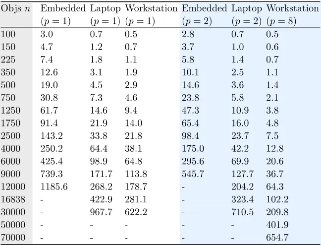
Table 1: Runtime (seconds) to check 600 seconds of orbit time. Objsn Embedded Laptop Workstation Embedded Laptop Workstation

(p= 1) (p= 1) (p= 1) (p= 2) (p= 2) (p= 8)

100 3.0 0.7 0.5 2.8 0.7 0.5

150 4.7 1.2 0.7 3.7 1.0 0.6

225 7.4 1.8 1.1 5.8 1.4 0.7

350 12.6 3.1 1.9 10.1 2.5 1.1

500 19.0 4.5 2.9 14.6 3.6 1.4

750 30.8 7.3 4.6 23.8 5.8 2.1

1250 61.7 14.6 9.4 47.3 10.9 3.8

1750 91.4 21.9 14.0 65.4 16.0 4.8

2500 143.2 33.8 21.8 98.4 23.7 7.5

4000 250.2 64.4 38.1 175.0 42.2 12.8

6000 425.4 98.9 64.8 295.6 69.9 20.6

9000 739.3 171.7 113.8 545.7 127.7 36.7

12000 1185.6 268.2 178.7 - 204.2 64.3

16838 - 422.9 281.1 - 323.4 102.2

30000 - 967.7 622.2 - 710.5 209.8

50000 - - - 401.9

70000 - - - 654.7

not being a perfect sphere, atmospheric drag, the gravity of the Moon and Sun, solar radiation, and other effects. Since these will modify more than one orbital element, other methods would be needed to computeocc-int, such as those based on reachability [4]. Still, even our Kepler approach could be considered as a broad-phase pass to detect potentially-colliding objects for further analysis with the more accurate propagation methods.

In the original benchmark proposal [10], satellites were initialized using uniform random values for their orbital elements rather than TLE sets, and only a regular 3D AABB tree approach was evaluated, although global variable time steps were considered. The 4D AABB approach is more efficient because it permits each object to have an individual time step.

6

Conclusion

Acknowledgments

Effort sponsored in whole or in part by the Air Force Research Laboratory, USAF, under Mem-orandum of Understanding/Partnership Intermediary Agreement No. FA8650-18-3-9325. The U.S. Government is authorized to reproduce and distribute reprints for Government purposes notwithstanding any copyright notation thereon. The views and conclusions contained herein are those of the authors and should not be interpreted as necessarily representing the official policies or endorsements, either expressed or implied, of the Air Force Research Laboratory.

References

[1] Stanley Bak and Kerianne Hobbs. Efficient n-to-n collision detection for space debris using 4D AABB trees (extended report). arXiv:1901.10475, 2019. https://arxiv.org/abs/1901.10475. [2] Gino van den Bergen. Efficient collision detection of complex deformable models using aabb trees.

Journal of graphics tools, 2(4):1–13, 1997.

[3] Angel P Del Pobil, Miguel A Serna, and Juan Llovet. A new representation for collision avoid-ance and detection. InRobotics and Automation, 1992. Proceedings., 1992 IEEE International Conference on, pages 246–251. IEEE, 1992.

[4] Parasara Sridhar Duggirala, Chuchu Fan, Matthew Potok, Bolun Qi, Sayan Mitra, Mahesh Viswanathan, Stanley Bak, Sergiy Bogomolov, Taylor T. Johnson, Luan Viet Nguyen, Christian Schilling, Andrew Sogokon, Hoang-Dung Tran, and Weiming Xiang. Tutorial: Software tools for hybrid systems verification, transformation, and synthesis: C2e2, hyst, and tulip. InProceedings of the Multi-Conference on Systems and Control. IEEE, 2016.

[5] A Foisy and V Hayward. A safe swept volume method for collision detection. InInternational Symposium of Robotics Research, pages 62–68, 1994.

[6] Elmer G Gilbert and SM Hong. A new algorithm for detecting the collision of moving objects. InRobotics and Automation, 1989. Proceedings., 1989 IEEE International Conference on, pages 8–14. IEEE, 1989.

[7] Stefan Gottschalk. Separating axis theorem. Technical report, Technical Report TR96-024, De-partment of Computer Science, UNC Chapel Hill, 1996.

[8] Stefan Gottschalk, Ming C Lin, and Dinesh Manocha. Obbtree: A hierarchical structure for rapid interference detection. InProceedings of the 23rd annual conference on Computer graphics and interactive techniques, pages 171–180. ACM, 1996.

[9] Steven A. Hildreth and Allison Arnold. Threats to u.s. national security interests in space: Orbital debris mitigation and removal. Technical report, Congressional Research Service, 101 Independence Ave, SE,Washington,DC,20540, 1 2014.

[10] Kerianne Hobbs, Peter Heidlauf, Alexander Collins, and Stanley Bak. Space debris collision detection using reachability. In5th International Workshop on Applied Verification of Continuous and Hybrid Systems, EPiC Series in Computing. EasyChair, 2018.

[11] Luc Jaulin. Applied interval analysis: with examples in parameter and state estimation, robust control and robotics, volume 1. Springer Science & Business Media, 2001.

[12] Pablo Jim´enez, Federico Thomas, and Carme Torras. 3d collision detection: a survey. Computers & Graphics, 25(2):269–285, 2001.

[13] TS Kelso et al. Analysis of the iridium 33-cosmos 2251 collision. Advances in the Astronautical Sciences, 135(2):1099–1112, 2009.

[15] St´ephane Redon, Abderrahmane Kheddar, and Sabine Coquillart. Fast continuous collision detec-tion between rigid bodies. InComputer graphics forum, volume 21, pages 279–287. Wiley Online Library, 2002.

[16] Donald J. Trump. Space Policy Directive-3, National Space Traffic Management Policy. https://www.whitehouse.gov/presidential-actions/ space-policy-directive-3-national-space-traffic-management-policy/, June 18, 2018. Presidential Memoranda.