Int. J. IndustrialMathematics (ISSN 2008-5621) Vol. 9, No. 4, 2017 Article ID IJIM-00812, 10 pages
Research Article
Numerical Solution of Fredholm Integro-differential Equations By
Using Hybrid Function Operational Matrix of Differentiation
R. Jafari ∗, R. Ezzati †‡, K. Maleknejad §
Received Date: 2016-03-21 Revised Date: 2016-08-01 Accepted Date: 2017-05-02
————————————————————————————————– Abstract
In this paper, first, a numerical method is presented for solving a class of linear Fredholm integro-differential equation. The operational matrix of derivative is obtained by introducing hybrid third kind Chebyshev polynomials and Block-pulse functions. The application of the proposed operational matrix with tau method is then utilized to transform the integro-differential equations to the alge-braic equations. Finally, show the efficiency of the proposed method is indicated by some numerical examples.
Keywords : Fredholm integro-differential equation; Hybrid function; Chebyshev polynomial; Block-pulse function; Operational matrix of derivative.
—————————————————————————————————–
1
Introduction
I
nest in the integro-differential equations, whichrecent years, there has been a growing inter-provide an important tool for modeling numer-ous real world problem in engineering, mechan-ics, physmechan-ics, chemistry, astronomy, biology, eco-nomics, potential theory and electrostatics. The kinds of equations are usually difficult to solve an-alytically, so it is required to obtain an efficient approximate solution. Therefore, many different methods are used to obtain the solution of the linear and nonlinear Integro-differential equations such as: the successive approximations, Adomian decomposition, Homotopy perturbation method,∗Department of Mathematics, Karaj Branch, Islamic Azad University, Karaj, Iran.
†Corresponding author. ezati@ kiau.ac.ir, Tel: +98(912)3618518
‡Department of Mathematics, Karaj Branch, Islamic Azad University, Karaj, Iran.
§Department of Mathematics, Karaj Branch, Islamic Azad University, Karaj, Iran.
Chebyshev and taylor collocation, Hybrid func-tion, Cas and Haar wavelet, Tau and Walsh series methods [1]-[8].
In this paper, a numerical method using hybrid of third kind Chebyshev polynomials and Block-pulse functions (HTKCPBPF) is presented for the following linear Fredholm integro-differential equations of the type:
u′(x) =f(x) +u(x) +λ∫01K(x, t)u(t)dt,
u(0) =a,
(1.1) where λ, a, are constants, f(x)) and K(x, t) are Known and u(t) is the unknown function to be determined. This method reduces the integral equation to a set of algebraic equations by ex-panding u(x) as (HTKCPBPF) with unknown coefficients. The paper is organized as follows: In Section2, we review briefly about Block-pulse functions and third kind Chebyshev polynomials and hybrid of them. Section3is devoted to func-tion approximafunc-tion. In Secfunc-tions 4, we construct
the operational matrices of derivative based on the (HTKCPBPF). Convergence analysis of the proposed method is done in Section5. In Section
6 and 7, we show the validity and efficiency of the proposed method, we present some numerical examples. Finally, Section8concludes the paper.
2
Function and hybrid function2.1 Block-pulse functions
A set of Block-pulse functions bi(x), i = 1,2, ..., N, on the interval [0,1) are defined as [9]:
bi(x) =
1, i−N1 ≤x < Ni
0, otherwise,
(2.2)
These functions satisfy in the following proper-ties:
i- disjointness
bi(x)bj(x) =
bi(x), f ori=j
0, f ori̸=j
ii- orthogonality
∫ 1
0
bi(x)bj(x)dt=
1
Nδij
where i, j = 1,2, ..., N, and δij is the Kronecker delta,
iii- completeness
for every f ∈ L2[0,1) when m approach to the infinity, parsevals identity hold:
∫ 1
0
f2(x)dx=
∞
∑
0
(fi2∥bi(x)∥2),
wherefi =N
∫1
0 f(x)bi(x)dx.
2.2 Third kind of Chebyshev polyno-mials
The third kind of Chebyshev polynomialVn(x) is
a polynomial of degree ninx defined by [9] :
Vn(x) =
cos(n+12)θ
cos(12)θ , (2.3)
where x = cosθ. clearly from 2.2, fundamental recurrence relation as follows:
Vn(x) = 2xVn−1(x)−Vn−2(x), n= 2,3, ...,
where
V0(x) = 1, V1(x) = 2x−1,
These polynomials are orthogonal on [−1,1] with
respect to the weight functionω(x) =
√
1+x
1−x, that
is ∫
1
−1
Vi(x)Vj(x)w(x)dx=πδij.
2.3 Hybrid functions
For n = 1, ..., N and m = 0, ..., M − 1, the HTKCPBPF are defined as follows [13]:
φnm(x) =
√
2
NVm(2N x−2n+ 1), n−1
N ≤x < n N
0, otherwise,
(2.4)
with the following weight function
ωn(x) =ω(2N x−2n+ 1).
3
Function approximation
A function f(x)∈L2[0,1) may be expanded as:
f(x) =
∞
∑
n=1
∞
∑
m=0
cnmφnm(x), (3.5)
where
cnm= ⟨f(x), φnm(x)⟩
⟨φnm(x), φnm(x)⟩
(3.6)
= N 2
π
∫ 1
0
In 3.6, ⟨., .⟩L2
ω[0,1) denotes the inner product in L2ω[0,1), with weight function wn(x). If the infi-nite series in 3.5 is truncated, then equation 3.5
can be written as:
f(x)≃
N
∑
n=1
M∑−1
m=0
cnmφnm(x) =CTφ(x), (3.7)
whereC andφ(x) areN M×1 matrices given by:
C= [c10, c11, c12, ..., c1,M−1, c20, ..., cN,M−1]T, (3.8)
φ(x) = [φ10(x), φ11(x), ..., φ1,M−1(x), φ20(x) (3.9)
..., φN,M−1(x)]T.
The differentiation of vector φ(x) can be ob-tained by:
dφ(x)
dx =Dφ(x). (3.10)
We derive the matrix D in the following section for some particular values ofN and M.
4
Operational matrix of
deriva-tive
In this section, we figure out the precise derivative of the HTKCPBPF withN = 2 and M = 3 . In this case, the six basis functions are given by :
φ1=φ10(x) = 1,
φ2=φ11(x) = 8x−3,
φ3=φ12(x) = 64x2−40x+ 5, (4.11)
fort∈[0,12),and
φ4=φ20(x) = 1,
φ5=φ21(x) = 8x−7,
φ6=φ22(x) = 64x2−104x+ 41, (4.12)
for t ∈ [12,1) . Let φ6(t) = (φ10(t) φ11(t) φ12(t) φ20(t) φ21(t) φ22(t)).
By differentiation 4.12, 4.13 from 0 to t, and
representing them in the matrix form, we obtain
dφ1
dx = 0, dφ2
dx = 8 = 8φ10, dφ3
dx = 128x−40 = 16φ11+ 8φ10, dφ4
dx = 0, dφ5
dx = 8 = 8φ20, dφ6
dx = 128x−104 = 16φ21+ 8φ20.
Thus, we have
dφ(x)
dx =D6×6φ(x). (4.13)
Where
D6×6= 2
0 0 0 0 0 0 4 0 0 0 0 0 4 8 0 0 0 0 0 0 0 0 0 0 0 0 0 4 0 0 0 0 0 4 8 0
The matrix D6×6 can be written as
D6×6= 2
[
F3×3 03×3 03×3 F3×3
]
where
F3×3 =
04 00 00 4 8 0
In general, for M ≥4, we have
dφ(x)
dx =Dφ(x), (4.14)
whereφ(x) is given in3.10and D is aN M×N M
matrix given by
D=N
F 0 0 · · · 0
0 F 0 · · · 0
0 0 F · · · 0
..
. ... ... . .. ...
0 0 0 · · · F
,
where F = a(ij) is M ×M matrices, whose the elements are given explicitly by:
aij =
2(i+j−1), i > j,(i+j)odd,
2(i−j), i > j,(i+j)even,
0, otherwise.
For example if M = 7 as follows: F =
0 0 0 0 0 0 0
4 0 0 0 0 0 0
4 8 0 0 0 0 0
8 4 12 0 0 0 0
8 12 4 16 0 0 0
12 8 16 4 20 0 0
12 16 8 20 4 24 0
7×7
,
Using the above procedure, the operational ma-trix ofnth derivative can be derived as:
dnφ(x)
dxn =D
nφ(x), (4.16)
The integration of two HTKCPBPF vectors is ob-tained as
E =
∫ 1
0
φ(t)φ(t)Tdt, (4.17)
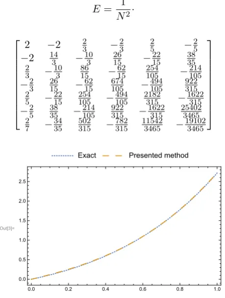
whereE is aN M×N M symmetric matrix. For example ifN = 1 andM = 6 as follows:
E= 1
N2·
2 −2 23 −23 25 −25
−2 143 −103 2615 −2215 3835 2 3 − 10 3 86 15 − 62 15 254 105 − 214 105 −2 3 26 15 − 62 15 674 105 − 494 105 922 315 2 5 − 22 15 254 105 − 494 105 2182 315 − 1622 315 −2 5 38 35 − 214 105 922 315 − 1622 315 25402 3465 2 7 − 34 35 502 315 − 782 315 11542 3465 − 19102 3465 Out[3]=
Exact Presented method
0.0 0.2 0.4 0.6 0.8 1.0
0.0 0.5 1.0 1.5 2.0 2.5
Figure 1: The exact and Presented method solu-tion of Example7.2
5
Convergence analysis
The following theorem gives the convergence and accuracy estimation of HTKCPBPF.
Out[81]=
Exact Presented method
0.0 0.2 0.4 0.6 0.8 1.0
0 5 10 15 20
Figure 2: The exact and Presented method solu-tion of Example7.3
Out[136]=
Exact Presented method
0.0 0.2 0.4 0.6 0.8 1.0
0.0 0.1 0.2 0.3 0.4 0.5 0.6 0.7
Figure 3: The exact and Presented method solu-tion of Example7.4
Theorem 5.1 Let f(x) be a second-order derivative square-integrable function defined on
[0,1) with bounded second-order derivative, say |f′′(x)|≤A for some constant A, then
(i) f(x) can be expanded as an infinite sum of the HTKCPBPF and the series converges to f(x) uniformly, that is
f(x) =
∞ ∑ n=1 ∞ ∑ m=0
cnmφnm(t),
where cnm=⟨f(x), φnm(x)⟩L2 ω[0,1).
(ii)
βf,n,M ≤ πA
2
8
∞
∑
n=N+1
∞
∑
m=M
1
n5(m−1)4,
where
βf,n,M =
[
∫ 1
0
|f(x)−
N
∑
n=1
M∑−1
m=0
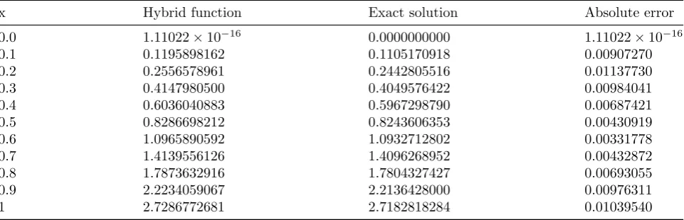
Table 1: shows some valuse of the solutions and absolute errors
x Hybrid function Exact solution Absolute error
0.0 1.11022×10⁻¹⁶ 0.0000000000 1.11022×10⁻¹⁶
0.1 0.1195898162 0.1105170918 0.00907270
0.2 0.2556578961 0.2442805516 0.01137730
0.3 0.4147980500 0.4049576422 0.00984041
0.4 0.6036040883 0.5967298790 0.00687421
0.5 0.8286698212 0.8243606353 0.00430919
0.6 1.0965890592 1.0932712802 0.00331778
0.7 1.4139556126 1.4096268952 0.00432872
0.8 1.7873632916 1.7804327427 0.00693055
0.9 2.2234059067 2.2136428000 0.00976311
1 2.7286772681 2.7182818284 0.01039540
Table 2: shows some valuse of the solutions and absolute errors
x Hybrid function Exact solution Absolute error
0.0 1 1 0
0.2 1.7471755121 1.8221188003 0.074943679
0.4 3.3022086903 3.3201169222 0.017908232
0.6 5.9881829326 6.0496474644 0.061464531
0.8 10.917173846 11.023176380 0.106002533
1 19.990251205 20.085536923 0.095285717
Table 3: shows some valuse of the solutions and absolute errors
x Hybrid function Exact solution Absolute error
0.0 1.14492×10⁻¹⁶ 0.0000000000 1.4492×10⁻¹⁶
0.2 0.1820778778 0.1823215567 0.000243679
0.4 0.3363045784 0.3364722366 0.000167658
0.6 0.4696357572 0.4700036292 0.000367872
0.8 0.5872265339 0.5877866642 0.000560131
1 0.6924314924 0.6931471805 0.000715688
Proof. To prove (i), we have:
(i)cnm =⟨f(x), φnm(x)⟩L2 ω[0,1)
= N 2
π
∫ 1
0
ωn(x)φnm(x)f(x)dx
= N 2
π
∫ n
N
n−1 N
f(x)
√
2
NVm(2N x−2n+ 1)
ω(2N x−2n+ 1)dx.
Lett= (2N x−2n+ 1) thendt= 2N dx. Clearly, we have
cnm = N
2π
√
2
N
∫ 1
−1
f(t+ 2n−1 2N )Vm(t)
√
1 +t
1−tdt.
By letting t = cosθ and the definition of the HTKCPBPF, it follows that
cnm = N 2π
√
2
N
∫ π
0
f(cosθ+ 2n−1
2N )
(cos mθ+cos(m+ 1)θ)dθ
= N 2π
√
2
N[
∫ π
0
f(cosθ+ 2n−1
2N )cos mθ
+
∫ π
0
f(cosθ+ 2n−1
2N )cos(m+ 1)θdθ].
Using the integration by parts, we have
cnm=
√
2
N
1 4π[
1
m
∫ π
0
f′(cosθ+ 2n−1
2N )
1
m+ 1
∫ π
0
f′(cosθ+ 2n−1
2N )
(sin(m+ 1)θsinθ)dθ] =
√
2
N
1
4π[I1+I2],
(5.18)
where
I1= 1
m
∫ π
0
f′(cosθ+ 2n−1
2N )
(sin mθsinθ)dθ,
and
I2= 1
m+ 1
∫ π
0
f′(cosθ+ 2n−1
2N )
(sin(m+ 1)θsinθ)dθ.
Now, we estimateI1 and I2, respectively. A sim-ple computation shows that
I1 = 1 2m
∫ π
0
f′(cosθ+ 2n−1
2N )
[cos(m−1)θ−cos(m+ 1)θ]dθ
= 1 2m
∫ π
0
f′(cosθ+ 2n−1
2N )
[cos(m−1)θdθ− 1
2m
∫ π
0
f′(cosθ+ 2n−1
2N )
cos(m+ 1)θ]dθ=I11−I12,
where
I11= [ 1 2m
∫ π
0
f′(cosθ+ 2n−1
2N )
cos(m−1)θdθ,
and
I12= 1 2m
∫ π
0
f′(cosθ+ 2n−1
2N )
cos(m+ 1)θdθ.
By using the integration by parts, and form >1, we get
I11=
1 4mN(m−1)
∫ π
0
f′′(cosθ+ 2n−1
2N )
[sin(m−1)θsinθ]dθ
= 1
8mN(m−1)
∫ π
0
f′′(cosθ+ 2n−1
2N )
[cos(m−2)θdθ−cos mθ]dθ,
I12=
1 4mN(m+ 1)
∫ π
0
f′′(cosθ+ 2n−1
2N )
[sin(m+ 1)θsinθ]dθ
= 1
8mN(m+ 1)
∫ π
0
f′′(cosθ+ 2n−1
2N )
[cos mθ−cos(m+ 2)θ]dθ.
Thus, form >1,we conclude that
I1= 1 8mN
∫ π
0
f′′(cosθ+ 2n−1
2N )
[cos(m−2)θ−cos mθ
(m−1) −
cos mθ−cos(m+ 2)θ
(m+ 1) ]dθ,
and hence
|I1|2=| 1 8mN
∫ π
0
f′′(cosθ+ 2n−1
2N )
[cos(m−2)θ−cos mθ
(m−1) −
cos mθ−cos(m+ 2)θ
(m+ 1) ]dθ| 2
= 1
64m2N2|
∫ π
0
f′′(cosθ+ 2n−1
2N )
[cos(m−2)θ−cos mθ
(m−1) −
cos mθ−cos(m+ 2)θ
By the fact that |f′′(x)|≤ A and Schwartz in-equality, it follows that
|I1|2≤
πA2
64m2N2(m−1)2(m+ 1)2
∫ π
0
|(m+ 1)cos(m−2)θ+ 2mcos mθ+
(m−1)cos(m+ 2)θ|2dθ
= πA
2
64m2N2(m−1)2(m+ 1)2×
[
∫ π
0
(m+ 1)2cos2(m−2)θdθ+
∫ π
0
4m2cos2mθdθ+
∫ π
0
(m−1)2cos2(m+ 2)θdθ]
= πA
2
64m2N2(m−1)2(m+ 1)2
[π
2(m+ 1) 2+π
24m 2+π
2(m−1) 2]
= π
2A2(3m2+ 1)
64m2N2(m−1)2(m+ 1)2
≤ π2A2
4N2(m−1)4.
Form >2, we obtain
|I1|≤
πA
2N(m−1)2 (5.19)
In a similar way, we will have
|I2|≤
πA
2N(m−1)2 (5.20)
Therefore, for m >2, we conclude that
|cnm|=|
1 4π
√
2
N[I1+I2]|
≤ 1
4π
√
2
N
πA N(m−1)2 ≤
A
2√2 1
n32(m−1)2
(5.21)
Note that f′(x) is bounded on [0,1) due to the fact that |f′′(x)|≤ A, indeed, by the Differential Mean Value Theorem and for anyt∈(0,1), there exists someγx∈(0, x) such that
f′(x)−f′(0) =f′′(γx)x,
So
|f′(x)|≤ |f′(0)|+A,
forx∈(0,1). Thusf′(x) is bounded on [0,1),say
|f′(x)|≤A˜ for some constant ˜A. Hence, by 5.18, we have
|cn,1|≤
√
2
N
1 4π[
∫ π
0
|f′(cosθ+ 2n−1 2N )|dθ
+1 2
∫ π
0
|f′(cosθ+ 2n−1 2N )|dθ]
=
√
2
N
1 4π
3 2
∫ π
0
|f′(cosθ+ 2n−1 2N )|dθ
≤
√
2
N
1 4π
3πA˜
2 =
3 ˜A
4√2n12
(5.22)
and
|cn,2|≤
√
2
N
1 4π[
1 2
∫ π
0
|f′(cosθ+ 2n−1 2N )|dθ
+1 3
∫ π
0
|f′(cosθ+ 2n−1 2N )|dθ]
=
√
2
N
1 4π
5 6
∫ π
0
|f′(cosθ+ 2n−1 2N )|dθ
≤
√
2
N
1 4π
5πA˜
6 =
5 ˜A
12√2n12
(5.23)
Relations 5.21-5.23 show that the series∑∞n=1∑∞m=0cnm is absolutely convergent. For m = 0 and according to the definition of
(ii)
βf,n,M2 =
∫ 1
0
|f(x)−
N
∑
n=1
M∑−1
m=0
cnmφnm(x)|2ωn(x)dx
=
∫ 1
0
| ∑∞ n=N+1
∞
∑
m=M
ynmφnm(x)|2ωn(x)dx
=
∞
∑
n=N+1
∞
∑
m=M |ynm|2·
(
√
2
N)
2
∫ n
N
n−1 N
Vm(2N x−2n+ 1)2·
√
1 + (2N x−2n+ 1) 1−(2N x−2n+ 1)dx.
Lett= 2N x−2n+ 1 thendt= 2ndx.
Therefore
βf,n,M2 =
∞
∑
n=N+1
∞
∑
m=M
|cnm|2 1 N2
∫ 1
−1
Vm2(t)
√
1 +t
1−tdt,
we have
∫ 1
−1
Vm2(t)
√
1 +t
1−tdt=π,
where the last equality follows due to the orthog-onality ofφnm(x). Together with5.21 we get
βf,n,M2 ≤ πA
2
8
∞
∑
n=N+1
∞
∑
m=M
1
n5(m−1)4.
6
Solution of Fredholm integro-differential equationConsider the linear Fredholm integro-differential equation given by 1.1. We approximate
u(x),K(x, t) ,f(x) by the way mentioned in sec-tion 2as:
u(x) =CTφ(x), K(x, t) =φT(x)Kφ(t),
f(x) =FTφ(x), (6.24)
by using 4.14we have
u′(x) =CTDφ(x). (6.25)
With substituting in 1.1we have
CTDφ(x) =FTφ(x) +CTφ(x)+
∫ 1
0
φT(x)Kφ(t)φT(t)Cdt. (6.26)
Applying 4.16, the residual R(x) for 1.1 can be written as:
R(x) =CTDφ(x)−FTφ(x)−CTφ(x)−
φT(x)KEC. (6.27)
As in a typical Tau method, we generateN M−1 linear equations by applying
∫ 1
0
ω(x)R(x)φi(x)dx= 0, ı = 0,1, ..., N M −1.
(6.28) Also, by substituting initial conditions 1.1 we have
u(0) =CTφ(0) =a, (6.29)
Eqs. 6.28-6.29 generate N M set of linear equa-tions. These linear equations can be solved for unknown coefficients of the vector C.
7
Numerical Examples
In this Section, linear Fredholm integro-differential equation have been solved using the proposed method.
Example 7.1 Consider the integro-differential equation
u′(x) = 1−13x+∫01xtu(t)dt,
u(0) = 0.
(7.30)
with the exact solution u(x) = x. We apply the method that was explained in Section 6 forN = 1, M = 3. After performing some manipulations, the components of the vectorC are given by
u(x) =CTφ(x).
c0= 3
4√2, c1 = 1
4√2, c2 = 0. Thus
u(x) =c0φ0(x) +c1φ1(x) +c2φ2(x) (7.31)
=
(
3 4√2
1 4√2 0
)
·
√
2
√
2(4x−3)
√
2(16x2−20x+ 5)
=x, (7.32)
Example 7.2 Consider the integro-differential equation
u′(x) =xex+ex−x+∫01xu(t)dt,
u(0) = 0.
(7.33)
with the exact solutionu(x) =xex. We apply the method that was explained in Section 6 forN = 1, M = 4. After performing some manipulations, the components of the vectorC are given by
c0 = 1.24557, c1= 0.564918,
c2= 0.106836, c3= 0.012142,
Thus
u(x) = 1.11022×10⁻¹⁶+
1.13549x+ 0.494223x2+ 1.09897x3. (7.34)
Table 1 shows some values of the solutions and absolute errors at some x, and plot of the exact and approximate solutions are shown in Figure1.
Example 7.3 Consider the integro-differential equation
u′(x) = 3e3x− 13(2e3+ 1)x+∫013xtu(t)dt,
u(0) = 1.
(7.35)
with the exact solutionu(x) =e3x. We apply the method that was explained in Section 6 forN = 1, M = 5. After performing some manipulations, the components of the vectorC are given by
c0 = 8.27245, c1= 4.1692,
c2 = 1.32412, c3= 0.312728,
c4 = 0.0567528.
Thus
u(x) =1 + 1.26846x+ 15.1003x2−
17.9252x3+ 20.5467x4. (7.36)
Table 2 shows some values of the solutions and absolute errors at some x, and plot of the exact and approximate solutions are shown in Figure2.
Example 7.4 Consider the integro-differential equation
u′(x) = u(x)−21x+1+1x−ln(1 +x)+ 1
(ln2)2
∫1 0
x
1+ty(t)dt, u(0) = 0,
(7.37)
with the exact solution u(x) = ln(1 +x). We apply the method that was explained in Section 6 for N = 1, M = 5. After performing some manipulations, the components of the vector C
are given by
c0 = 0.38715, c1 = 0.110789,
c2 =−0.00924358, c3 = 0.00105708,
c4 =−0.000129514.
Thus
u(x) = 1.14492×10⁻¹⁶+ 0.993861x−
0.455717x2+ 0.201176x3−0.046889x4.
(7.38)
Table 3 shows some values of the solutions and absolute errors at some x, and plot of the exact and approximate solutions are shown in Figure3.
8
Conclusion
In this paper, we constructed operational matrix of derivative of hybrid the third kind Chebyshev polynomials and Block-pulse functions. Also, we applied these matrices to convert Fredholm integro-differential equations to system of linear algebraic equations. As to validity and efficiency of the proposed method, we presented some nu-merical examples.
References
[1] S. H. Behiry, Solution of nonlinear Fredholm integro-differential equations using a hybrid of Block pulse functins and normalized Bern-stein polynomials,Comput. Appl. Math.260 (2014)258-265
[2] H. Danfu, Sh. Xufeng, Numerical solution of integro-differential equations by using CAS wavelet operational matrix of integration,
Appl. Math. Comput.194 (2007) 460-466
[4] P. Darania, A. Ebadian, A method for the numerical solution of the integro-differential equations, Appl. Math. Comput.
(2006), http://doi:10.1016/j.amc.2006. 10.046/.
[5] R. Ezzati, S. Najafalizadeh, Numerical solu-tion of nonlinear Volterra-Fredholm integral equation by using Chebyshev polynomials,
Appl. Math. Comput.(2003) 1530-1539.
[6] A. Golbabai, M. Javidi, Application of He’s homotopy perturbation method for nth-order integro-differential equations, Appl. Math. Comput.190 (2007) 1409-1416.
[7] J. Hou, Ch. Yang, Numerical method in solv-ing Fredholm integro-differential equations by using hybrid functin operational matrix of derivative,Journal of Information and Com-putational Science (2013) 2757-2764
[8] H. Jaradat, O. Alsayyed, S. Al-Shara, Nu-merical solution of linear integro-differential equations, Journal of Mathematics and Statistics 11 (2008) 250-254.
[9] Z. H. Jiang, W. Schaufelberger, 1991, Block-pulse Functions and their Applications in Contorl Systems, Springer-Verlag Berlin Heidelberg New York 37.
[10] A. Karamete, M. Sezer, A Taylor colloca-tion method for the solucolloca-tion of linear integro-differential equations,Int. J. Comput. Math.
79 (2002) 987-1000
[11] S. J. Liao, An explicit analytic solution to the Thomas-Fermi equation, Appl. Math. Comput.144 (2003) 495-506
[12] K. Maleknejad, F. Mirzaee, Numerical solu-tion of integro-differential equasolu-tions by using rationalized Haar functions method, Kyber-netes, Int. J. Syst. Math. 35 (2006) 1735-1744
[13] K. Maleknejad, M. Tavassoli Kajani, A hy-brid collocation metod based on combining the third kind Chebyshev polynomials and Block-pulse functions for solving higer-order initial value problems,Kuwait journal of Sci-ence (2016).
[14] J. C. Mason, D. C. Handscomb, Chebyshev polynomials (2002) ISBN:0-8493-0355-9.
[15] S. Yeganeh, Y. Ordokhani, A. Saadatmandi, A Sinc-collocation method for second-order boundary value problems of nonlinear integro-differential equation,J. Inf. Comput. Sci.7 (2012) 151-160.
Reza Jafari was born in Miandoab, Iran, in 1976. He obtained his M.Sc degree in Applied Mathemat-ics from Islamic Azad University Karaj Branch, Iran, in 2007 and he is currently Ph.D. Student in IAU-Karaj branch. Also he is one of the researcher in this university.
R. Ezzati received his PhD degree in applied mathematics from IAU-Science and Research Branch, Tehran, Iran in 2006. He is an pro-fessor in the Department of Mathe-matics at Islamic Azad University, Karaj Branch, (Iran) from 2015. He has published more than 120 papers in inter-national journals, and he also is the associate ed-itor of Mathematical Sciences (a Springer Open Journal). His current interests include numer-ical solution of differential and integral equa-tions, fuzzy mathematics, especially, on solution of fuzzy systems, fuzzy integral equations, and fuzzy interpolation.