Design of obstacle avoidance controller for agricultural tractor based on
ROS
Zhengduo Liu
1,2,
Zhaoqin Lü
1,2,
Wenxiu Zheng
1,2*,
Wanzhi Zhang
1,2,
Xiangxun Cheng
1,2 (1. College of Mechanical and Electronic Engineering, Shandong Agricultural University, Tai’an 271018, China;2. Shandong Provincial Key Laboratory of Horticultural Machinery and Equipment, Tai’an 271018, China)
Abstract: The obstacle avoidance controller is a key autonomous component which involves the control of tractor system dynamics, such as the yaw lateral dynamics, the longitudinal dynamics, and nonlinear constraints including the speed and steering angles limits during the path-tracking process. To achieve the obstacle avoidance ability of control accuracy, an independent path re-planning controller is proposed based on ROS (Robot Operating System) nonlinear model prediction in this paper. In the design process, the obstacle avoidance function and an objective function are introduced. Based on these functions, the obstacle avoidance maneuvering performance is transformed into a nonlinear quadratic optimization problem with vehicle dynamic constraints. Moreover, the tractor dynamics maneuvering performance can be effectively adjusted through the proposed objective function. To validate the proposed algorithm, a ROS based tractor dynamics model and the SLAM (Simultaneous Localization and Mapping) are established for numerical simulations under different speed. The maximum obstacle avoidance deviation in the simulation is 0.242 m at 10 m/s, and 0.416 m at 30 m/s. The front-wheel rotation angle and lateral velocity are within the constraint range during the whole tracking process. The numerical results show that the designed controller can achieve the tractor obstacle avoidance ability with good accuracy under different conditions.
Keywords: ROS, obstacle avoidance, nonlinear model prediction, agricultural tractor
DOI: 10.25165/j.ijabe.20191206.4907
Citation: Liu Z D, Lü Z Q, Zheng W X, Zhang W Z, Cheng X X. Design of obstacle avoidance controller for agricultural tractor based on ROS. Int J Agric & Biol Eng, 2019; 12(6): 58–65.
1 Introduction
Path tracking of agricultural vehicles is the key technology for the automation and intelligence of agricultural machinery[1]. The obstacle avoidance ability of vehicles is an important indicator of the intelligence of vehicles. The obstacle avoidance system of agricultural vehicles involves two key technologies of precise positioning and path re-planning of vehicles[2-4].
For precise positioning, GPS positioning, image processing, ultrasonic positioning, and other technologies are widely used in agriculture[5-7]. Kayacan et al.[8] applied GPS and electronic
compass to achieve the automatic navigation of tractors, however, the GPS signal reception and positioning accuracy are not ideal. This is because the branches and leaves of fruit trees block the GPS receiver, making it unable to receive satellite signals stably. Meanwhile, Wei et al.[9] proposed a set of field obstacle detection system based on binocular vision. The proposed detection system can detect the obstacles higher than the canopy of the field crop and obtain the range and distance of the obstacle through stereo
Received date: 2019-01-10 Accepted date:2019-08-24
Biographies: Zhengduo Liu, PhD candidate, research interests: intelligent agricultural machinery, Email: [email protected]; Zhaoqin Lü, PhD, Professor, research interests: potato agricultural machinery, Email: [email protected]; Wanzhi Zhang, PhD, Lecturers, research interests: Intelligent and assisted driving of vehicles, Email: [email protected]. Xiangxun Cheng, Master candidate, research interests: intelligent agricultural machinery and equipment. Email: [email protected].
*Corresponding author: Wenxiu Zheng, PhD, research interests: potato
machinery and intelligent agricultural machinery. College of Mechanical and Electronic Engineering, Shandong Agricultural University, Tai’an 271018, China. Email: [email protected].
matching. Moreover, Nissimov et al.[10] investigated Kinect sensors and used it to detect inter-row obstacles in greenhouse crops by calculating the gradient of data. However, during the obstacles avoidance process in complex farmland environments, it is not possible to implement the algorithm in real-time.
Path re-planning algorithms can be roughly divided into global path planning algorithms and local path planning algorithms[11,12]. The global path planning algorithm has a large amount of computation, with poor real-time performance and dynamic performance. The local path tracking algorithm is the main method to realize the obstacle avoidance of agricultural vehicles. Wang et al.[13] proposed to use the fuzzy-logic algorithm to design the path planning controller. Although an optimal local path can be obtained, it may lead to no solution when dealing with multiple obstacles. Furthermore, Kerr et al.[14] constructed a global
continuous optimized trajectory with the local approximation based on spline method. However, with the increases in the dimension of the parameter space, the algorithm convergence speed is relatively slow.
From the current stage of agricultural navigation, Multi-sensor and multi-algorithm fusion technology have gained a lot of attention to improve efficiency during the obstacles detecting process. Meanwhile, in the design process of the obstacle avoidance controller, improving the control accuracy and the vehicle dynamic performance of the agricultural tractors still pose a challengeduring the trajectory following maneuvering[11,15,16].
proposes a pre-SLAM mapping of the tracking area, which further improves the positioning accuracy and real-time performance of agricultural vehicles[21-22]. Finally, the model predicted algorithm[23-26] is introduced during the trajectory tracking process.
Using the model predictive control algorithm, multiple constraints can be taken into considerations in the process of path planning to compensate for the modeling uncertainties, especially at high speed and complex road conditions.
2 Path re-planning controller
2.1 Tractor dynamics modeling
In order to design the path re-planning controller, the tractor vehicle dynamic model is needed to be established. A simplified tractor dynamic model[27-29] is illustrated in Figure 1. The lateral force, navigation angle, and yaw rate are considered in details in order to research the obstacle avoidance ability. As is shown in Figure 1, x is the forward speed (m/s); y is the lateral speed (m/s); ay is lateral acceleration (m/s2); φ is the tractor navigation
angle (rad); is the yaw rate (rad/s); δ is the navigation angle in the global coordinate (rad).
Figure 1 Schematic Diagram of the tractor mathematic model The mathematic model is given as follow, u=ay is the
0 / cos sin sin cos y y x y a a x X x y Y x y
(1)
To rewrite the model in state space form, take
T
=[ , , , ,x y Y X]
as the state variables, u=ay is the control variable
in the following form.
( )t f( ( ), )t u h
(2)
In which, the output vector is given by
T
1 0 0
[ , , , , ] , 0 1 0
0 0 1
x y Y X h
.
To implantation for real-time computation the controller in digital systems, the agricultural vehicle particle model is further discretized in (3).
( 1) ( )
( 1) ( ) * ( )
( 1) ( ) * ( ) / ( )
( 1) ( ) ( cos ( ) sin ( ))
( 1) ( ) * ( sin ( ) cos ( ))
y y
x k x k
y k y k T a k k k T a k x k
X k X k T x k y k Y k Y k T x k y k
(3)
In which, k is a discrete-time variable. According to this
mathematic model, it is necessary to know the initial information (x(k), y(k), φ(k), X(k), Y(k)) of the controlled system at a certain time and the control input sequence ay(k), ay(k+1) to predict the output
sequence of the system in the predicted k+1 time domain.
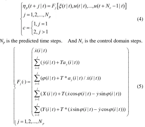
(4)
Np is the predicted time steps. And Nc is the control domain steps.
1 1 1 1 ( | ) ( ( | ) ( | )) ( ( | ) * ( | ) / ( | )) ( )
( ( | ) ( cos ( | ) sin ( | ))
( ( | ) * ( sin ( | ) cos ( | )))
1, 2,..., j y i j y i j j i j i p
x i t
y i t Ta i t
i t T a i t x i t F
X i t T x i t y i t
Y i t T x i t y i t
j N
(5)To reduce the computational complexity and enhance the real-time performance of the control system, this paper set Nc to 2.
Thus, the prediction model of nonlinear model predictive controller is obtained: r 1 2 r r r
( 1 ) ( )
( )
( 2 )
( ) , 1, 2,...,
( )
( )
( )
( | ) p
r p
j
N p
t t F F t t
t j N
F t j t
F t N t
(6)
In order to improve the robust performance of the control system, closed-loop correction of the prediction model is coined based on the error prediction and real-time feedback.
( 1| ) r( 1| )- p( 1| ), 1,2,..., p
e t i t t i t t i t i N (7) where, ηr(t+i–1|t) is the system output at t+i–1 based on the
real-time information measurement at t; ηp(t+i–1|t) is the output at
t+i–1 based on kinematics model of the agricultural vehicle at t.
2.2 Obstacle avoidance function
The paper proposes to construct the detection zone for the local re-planning path, as shown in Figure 2. The LIDAR is used to detect the position of the obstacle in the coordinate. This helps to improve the accuracy of path tracking and obstacles. The obstacle avoidance function is put forward to adjust the distance between the agricultural vehicle and the obstacle in real time trajectory tracking. As the tractor approaches near toward the obstacle, the obstacle function value will increase.
The obstacle avoidance function is given as follow,
2 2
0 1 0 1
( ) ( )
obj obs
S J
x x y y
(8)
where, Sobjis the weight coefficient; (x1, y1) is the coordinate value
of the obstacle and (x0, y0) is the center of gravity point of the
plan will increase. At this time, the path planned by the path re-planning controller will deviate from the reference path to avoid obstacles. When the agricultural vehicle is far away from the obstacle, the value of the obstacle avoidance function will decrease and the influence of the obstacle on the path plan will decrease. At this time, the agricultural vehicle will continue to travel along the reference path. The obstacle avoidance function value varies in the obstacle relative coordinate is shown in Figure 3.
Figure 2 Schematic Diagram of the control strategy \
Figure 3 Obstacle avoidance function value in obstacle coordinate
For any predicted steps Np, the objective function J(·,·) is
shown as follows,
1
1 0
( ) ( )
P
N Nc
T T
obs
i i
J Q u t R u t J
(9)where, Δu is the control input; Q, R are the weighting factor matrix, and ΔΓ is illustrated as follow,
T
( ) ( )=[ ( 1 ), , ( )]
r t p t e t t e t N tp
(10)
The first term of the objective function describes the tracking ability of the desired state variables. The second term characterizes the system input. And the third term illustrates the effect of the obstacle avoidance function. When there is no obstacle in front of the agricultural vehicle, the obstacle avoidance function value is 0, and the re-planning path is consistent with the reference path.
The path tracking problem is transformed to solve the constraint problem of nonlinear quadratic form by setting the value range of state quantity and control quantity. Both the objective function and the constraint function are continuous, and the gradient is continuous in Equation (9). Therefore, the objective optimization problem is can be solved based on quadratic programming of the recursive sequence. By taking the nonlinear boundary constraints into account, the optimization problem can be summarized as
1
2
1 0
( ) ( )+
P
N Nc
T T
i i
J Q u t R u t
s.t
min max
min max
min max
min max
( ) ( )
, 0,1, , 1
, 0,1, , 1
c c
t t
t k k N
t k k N
u u u
u u u
≤ ≤
≤ ≤
(11)
3 Tractor dynamics model and SLAM map
3.1 Tractor dynamics model
The dynamics simulation of the tractor requires the collection of a large number of tractor driving parameters. The ROS system is widely used in the unmanned field. It can combine the data collected by various sensors and use the open source function package to determine the driving parameters for the agricultural vehicle, which greatly simplifies the process of applying the driverless algorithm to the agricultural vehicle. The gazebo software under the ROS framework is mainly used to simulate the dynamics of robots[30,31]. Considering the complexity of the tractor structure, this paper adopts the method of multi-body system modeling to decompose the topology of the multi-body system into several independent chain subsystems. The specific structure used for later analysis is shown in Figure 4.
Figure 4 Tractor Configuration
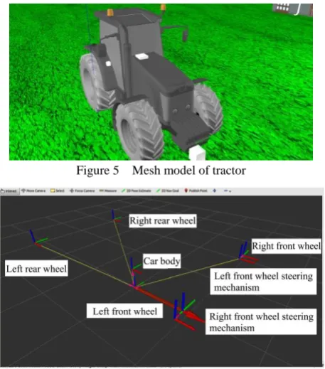
The tractor kinetic model of Figure 5 and the topological structure Figure 6 was established in ROS-gazebo.
Figure 5 Mesh model of tractor
3.2 SLAM map
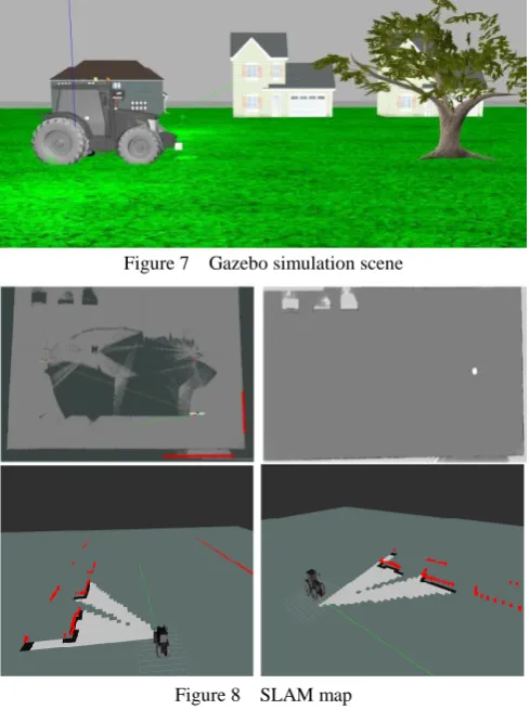
The paper uses SLAM to map the working area of the agricultural vehicle, that is, the two-dimensional map of the grid is established in advance by laser radar. It can make the agricultural vehicle locate its position and posture through repeated observation of map features (such as trees, pillars, etc.), and then construct the map incrementally according to its own position, thereby achieving the purpose of positioning and map construction. The simulation was carried out on the mapping environment. The mapping environment was shown in Figure 7, and the mapping process with SLAM is shown in Figure 8.
Figure 7 Gazebo simulation scene
Figure 8 SLAM map
In this paper, the grid mapping construction method based on particle filter algorithm is used. The algorithm combines coordinate transformation, speed and rotation angle information, and LiDAR detection information to draw a two-dimensional grid map. The planned trajectory is constructed based on it.
In order to further illustrate the effect of implementing SLAM mapping in the tracking area, Gaussian noise is added to the ROS-gazebo physical simulation environment for comparative simulation. The tractor advances 4 m at a speed of 1 m/s, then rotates 180°, and finally drives to the origin. The result is shown as follow.
It can be seen from Figure 9a that in the absence of SLAM construction, the tractor produces a large deviation at 5.6 s. At this time, it can be seen from Figure 10b that the tractor rotates 180 degrees and starts to travel to the origin. Since there is no external sensor to verify the position of the tractor, the vehicle will travel along the reference path, which will cause the cumulative deviation of the error with time.
However, as can be seen from Figure 9b, when the tractor with SLAM map rotates 180° at 5.4 s, it has a process of adjusting the front wheel angle. This is because the ROS with SLAM map detects the surrounding environment by laser radar, and compares
and analyzes with the SLAM map to obtain the right tractor position. Then, the tractor continues along the reference path with a small tracking deviation and finally drivers to the origin.
a. Lateral deviation
b. Navigation angle deviation Figure 9 SLAM map performance
4 Simulation and analysis
In the simulation, Matlab/Simulink runs the path re-planning algorithm, which collects the speed, rotation angle, position and other information of the tractor dynamics model in ROS-gazebo, and output the front wheel angle into the ROS-gazebo dynamic model. The ROS-gazebo toolbox mainly performs vehicle dynamic analysis and feedback the sensors’ information into Matlab. The vehicle used in the ROS-gazebo toolbox is shown in Table 1.Reference trajectory is shown in Figure10.
Figure 10 Reference trajectory
Table 1 Vehicle parameters
Technical Parameters Value
CG to front axle/mm 1016
CG to rear axle/mm 1526
Front tire lateral slip rate 0.2
Rear tire lateral slip rate 0.2
Front wheel lateral stiffness –67 000 Rear wheel lateral stiffness –63 000
as T=0.2 s, Np=25, Nc=2, Q=10*diag(1,1,…,1), R=5*diag(1,1,…,1).
The objective function parameters are set as follows:
min max
min
min max
max
3.2 0.5 , 3.2 0.5
1 1 0.5 , 22 12 0.5
0.05 0.05 0.0082 , 0.05 0.05 0.0082
T T
T T
T T
u u
4.1 The effect of speed on obstacle avoidance performance
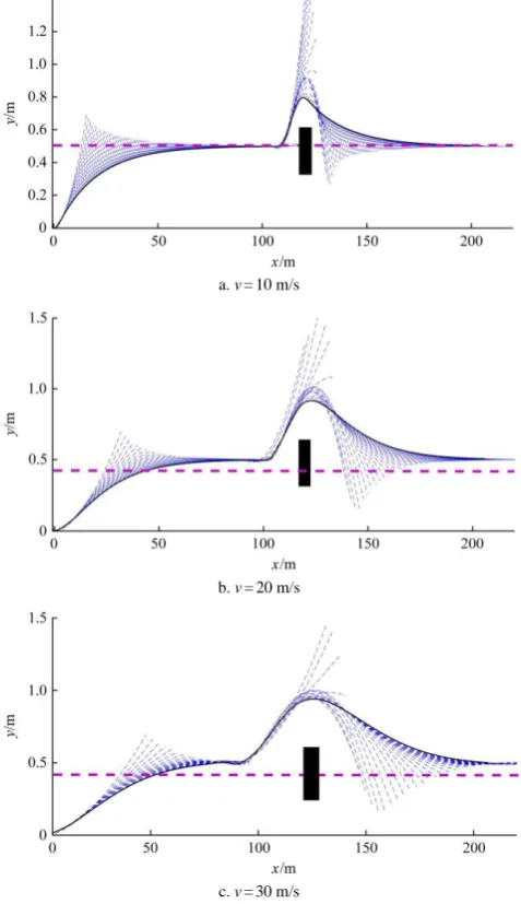
The linear reference trajectory (desired trajectory) is y=0.5 m, the tractor initial pose information is (0, 0, 0), and the linear trajectory tracking simulation effect is shown in Figure 11.
a. v=10 m/s
b. v=20 m/s
c. v=30 m/s
Figure 11 Obstacle avoidance simulation results From Figure 11, the tractor tracks the reference path and avoids the obstacle at different driving speeds with good robustness to speed. The tractor starts from the point where the vehicle does not perceive the existence of obstacles. The re-planning path coincides with the reference path. When the vehicle travels 90 m, the vehicle senses the obstacle at 30 m ahead, and the obstacle information is fed back to the re-planning controller. The trajectory of the tractor is re-planned, so that the trajectory of the agricultural vehicle deviates from the reference trajectory to avoid obstacles, and after that, the vehicle quickly tracks back to the reference trajectory.
As is shown in Figure 12, the tractor deviates from the reference trajectory when avoiding obstacles, resulting in a large lateral tracking deviation. The maximum lateral deviation is 0.242 m at
a speed of 10 m/s and reaches 0.416 m at a speed of 30 m/s. The maximum lateral deviation increases when the speed rises. After the avoidance trajectory, the lateral deviation gradually decreases toward zero. The longitude deviation also increases with a higher velocity due to the transient response of the vehicle. All in all, the designed obstacle avoidance controller can effectively preplan the new trajectory in case of the obstacles with accuracy even under different velocities.
a. Lateral distance deviation
b. Longitude distance deviation
c. Lateral speed
Figure 12 Tractor obstacle avoidance controller accuracy As is shown in Figure 13, the vehicle with the designed obstacle avoidance controller shows good maneuvering performance. All the vehicle dynamics parameters are within the constraint range of the objective function. The lateral acceleration of the tractor is kept within ±0.2 m/s2, and the navigation angle of the tractor is within ±0.8°. The dynamic performance of the vehicle is kept within the safety region with a good margin.
4.2 Effect of weight coefficient on obstacle avoidance performance
Figure 14 shows the path tracking results when the weighting factor Sobj changes from 10, 100, to 1000 respectively under a
speed of 20 m/s. It can be seen from Figure 14a that the obstacle avoidance behavior is completed at x=172.83 m, 186.96 m, and 199.82 m when Sobj is 10, 100, and 1000 respectively. When
increases the weighting factor Sobj, re-planning results tend to be
a. Front wheel angle b. Front wheel angle increment
c. Lateral speed d. Lateral acceleration
e. Side slip angle
Figure 13 Tracking stability analysis of tractor obstacle avoidance controller
a. Tracking trajectory b. Front wheel angle
c. Lateral speed
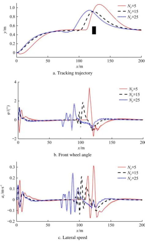
4.3 Influence of predicted time on obstacle avoidance performance
Figure 15 shows the path tracking results when the predicted time Np changes from 5, 15 to 25 respectively when forward speed
is 20 m/s and Sobj is 100. When Np=5, the maximum front wheel
angle of the tractor is 1.78°, and the maximum lateral speed is 0.285 m/s. Meanwhile, the maximum front wheel angle is 3.48° and the maximum lateral speed is 0.334 m/s when Np=25. As the
prediction time domain increases, the steering angle and the lateral velocity amplitude decreases, making the steering much smoother. The lateral distance deviation during obstacle avoidance maneuvering is reduced. This is reasonable since the controller can better predict the future trajectory and reacts even earlier by the steering angle. However, it will exert a large computation load for the controller when increases the prediction time.
a. Tracking trajectory
b. Front wheel angle
c. Lateral speed
Figure 15 Simulation results of tractor obstacle avoidance with the different predicted time
5 Conclusions
1) The mathematic model and the error predicted model of a tractor were established. By introducing an obstacle avoidance function and an objective function, obstacle avoidance maneuvering problem was transformed into a nonlinear quadratic optimization problem with speed and steering angle constraints.
2) The tractor dynamics model based on ROS-gazebo was established and a scheme of using SLAM to map the track area of agricultural vehicles was proposed. Then the joint simulation of
ROS-Simulink was realized. The controller was applied to the ROS-Simulink simulation to validate the proposed algorithm.
3) The simulation results showed that the controller designed in this paper can achieve reliable obstacle avoidance under different speeds and different control parameters with good maneuverability.
Acknowledgements
This work was supported by Shandong Agricultural Machinery and Equipment Research and Development Innovation Initiative (2018YF020-07, 2017YF002), Modern Agricultural Technology System Innovation Team Post Project in Shandong Province (SDAIT-16-10), the National Key Research Projects (2017 yfd0700705).
[References]
[1] Tian G Z. Research on the key techniques of intelligent agricultural vehicles navigation system. PhD dissertation. Nanjing: Nanjing Agricultural University, 2013.
[2] Reid J F, Zhang Q, Noguchi N, Dickson M. Agricultural automatic guidance research in North America. Computers & Electronics in Agriculture, 2000; 25(1): 155–167.
[3] Hilgert J, Hirsch K, Bertram T, Hiller M. Emergency path planning for autonomous vehicles using elastic band theory. Proc. 2003 IEEE/ASME International Conference on Advanced Intelligent Mechatronics, Kobe: Japan, 2003; 21(2): 1390–1395.
[4] Luo X W, Zhang Z G, Zhao Z X, Chen B, Hu L, Wu X P. Design of DGPS navigation control system for Dongfanghong X-804 tractor. Transactions of the CSAE, 2009; 25(11): 139–145. (in Chinese)
[5] Li Y J, Zhao Z X, Huang P, Guan W, Wu X. Automatic navigation system of tractor based on DGPS and double closed-loop steering control. Transactions of the CSAM, 2017; 48(2): 11–19. (in Chinese)
[6] Li T H, Wu Z H, Lian X K, Hou J L, Shi G Y Wang Q. Navigation line detection for greenhouse carrier vehicle based on fixed direction camera. Transactions of the CSAM, 2018; 49(S1): 8–13. (in Chinese)
[7] Hu J, Gao L, Bai X P, Li T C, Liu X. Review of research on automatic guidance of agricultural vehicles. Transactions of the CSAE, 2015; 31(10): 1–10. (in Chinese)
[8] Kayacan E, Kayacan E, Ramon H, Kaynak O, Saeys W. Towards agrobots: trajectory control of an autonomous tractor using type-2 fuzzy logic controllers. IEEE/ASME Transactions on Mechatronics, 2015; 20(1): 287–298.
[9] Wei J, Rovira-Mas F, Reid J F, Han S. Obstacle detection using stereo vision to enhance safety of autonmmous machines. Transactions of the ASAE, 2005; 48(6): 2389–2397.
[10] Nissimov S, Goldberger J, Alchanatis V. Obstacle detection in a greenhouse environment using the Kinect sensor. Computers & Electronics in Agriculture, 2015; 113: 104–115.
[11] Liu P Z, Bi S S, Zang G S, Wang W S, Gao Y S, Deng Z M. Obstacle avoidance system for agricultural robots based on multi-sensor information fusion. Proc. 2011 International Conference on Computer Science and Network Technology. Harbin: China, 2012; pp.1181–1185.
[12] Xin Y, Liang H W, Du M B, Mei T, Wang Z L, Jiang R H. An improved A* algorithm for searching infinite neighborhoods. Robot, 2014; 36(5): 627–633.
[13] Wang M, Liu J N K. Fuzzy logic based robot path planning in unknown environment. IEEE proceedings of 2005 International Conference on Machine Learning and Cybernetics, Guangzhou: China, 2005; pp.813–818. [14] Kerr J,Nickels K.Robot operating systems: Bridging the gap between human and robot. Proceedings of the 2012 44th Southeastern Symposium on System Theory (SSST), Jacksonville FL: USA, 2012; pp.99–104. [15] Ding X, Yan L, Liu J, Kong J, Yu Z. Obstacles detection algorithm in
forest based on multi-sensor data fusion. Journal of Multimedia, 2013; 8(6): 790–795.
[17] Wang Y, Yang F, Wang T, Liu Q, Xu X. Research on visual navigation and remote monitoring technology of agricultural robot. International Journal on Smart Sensing and Intelligent Systems, 2013; 6(2): 466–481. [18] Shamshiri R R, Hameed I A, Karkee M, Weltzien C. Automation in
Agriculture – Securing Food Supplies for Future Generations. InTechOpen. 2018; 43p.
[19] Shamshiri R R, Weltzein C, Hameed I A, Yule I J, Grift T E, Balasundram S K, et al. Research and development in agricultural robotics: A perspective of digital farming. Int J Agric & Biol Eng, 2018; 11(4): 1–14. [20] Shamshiri R R, Hameed I A, Pitonakova L, Weltzien C, Balasundram S K, Yule I J, et al. Simulation software and virtual environments for acceleration of agricultural robotics: Features highlights and performance comparison. Int J Agric & Biol Eng, 2018; 11(4): 15–31.
[21] Ortigoza R S, Sanchez J R G, Guzman V M H, Sanchez C M, Aranda M M. Trajectory tracking control for a differential drive wheeled mobile robot considering the dynamics related to the actuators and power stage. IEEE Latin America Transactions, 2016; 14(2): 657–664.
[22] Bauer R, Fels M, Vukelić M, Ziemann U, Gharabaghi A. Bridging the gap between motor imagery and motor execution with a brain-robot interface. Neuroimage, 2015; 108: 319–327.
[23] Ohnishi N, Imiya A. Visual navigation of mobile robot using optical flow and visual potential field. In Sommer G, Klette R. Ed. Lecture Notes in Computer Science, Springer, 2008; 4931: 412–426.
[24] Bai X P, Hu J T, Gao L, Liu X. Self-tuning model control method for
farm machine navigation. Transactions of the CSAM, 2015; 46(2): 1–7. (in Chinese)
[25] Zhang L X, Wu G Q, Guo X X. Path tracking using linear time-varying model predictive control for autonomous vehicle. Journal of Tongji University: Natural Science, 2016; 44(10): 1595–1603.
[26] Liu Z D, Zhang W Z, Lv Z Q, Zheng W X, Mu G Z. Design and Test of Path Tracking Controller Based on Nonlinear Model Prediction. Transactions of the CSAM, 2018; 49(7): 23–30. (in Chinese)
[27] Velenis E, Tsiotras P. Optimal velocity profile generation for given acceleration limits: the half-car model case. Proc. IEEE International Symposium Systems, 2005; pp.355–360.
[28] Gao Y, Lin T, Borrelli F, Tseng E, Hrovat D. Predictive control of autonomous ground vehicles with obstacle avoidance on slippery roads. Proceedings of the ASME 2010 Dynamic Systems and Control Conference, Cambridge MA, USA, 2010; pp.265–272.
[29] Gong J W, Jian Y, Xu W. Model predictive control for self-driving vehicles. Beijing Institute of Technology Press, 2014.
[30] Liu J, Jayakumar P, Stein J L, Ersal T. Combined speed and steering control in high speed autonomous ground vehicles for obstacle avoidance using model predictive control. IEEE Transactions on Vehicular Technology, 2017; 66(10): 8746–8763.