Using the Adaptive Frequency Nonlinear Oscillator for
Earning an Energy Efficient Motion Pattern in a Leg- Like
Stretchable Pendulum by Exploiting the Resonant Mode
M. R. Sayyed Noorani
1*, A. Ghanbari
2, M. A. Jafarizadeh
3 1- Ph.D Student. Faculty of Mechanical Engineering, University of Tabriz, Tabriz, Iran 2- Associate Porfessor, Faculty of Mechanical Engineering, University of Tabriz, Tabriz, Iran 3- Porfessor, Department of Theoretical Physics and Astrophysics, University of Tabriz, Tabriz, IranABSTRACT
In this paper we investigate a biological framework to generate and adapt a motion pattern so that can be energy efficient. In fact, the motion pattern in legged animals and human emerges among interaction between a central pattern generator neural network called CPG and the musculoskeletal system. Here, we model this neuro - musculoskeletal system by means of a leg - like mechanical system called stretchable pendulum, and an adaptive frequency nonlinear oscillator as a CPG unit. The stretchable pendulum is a simple oscillating mass - spring mechanism that interacts with the ground during its oscillations, and this interaction begins with a collision. Interaction with the ground causes the model to involve in two dynamic phases that are switched to each other through transition events. This hybrid model is very similar to models have been proposed for the legged locomotion mechanisms. Then, it will be simulated in coupling with an adaptive frequency Hopf oscillator as a controller placed in feedback loop. The simulation results reveal that this scheme is able to excite the mechanical system in an energy efficient pattern by way of exploiting resonance phenomenon. Also, adaptation of the system against the environmental changes is examined and it is seen that the controller is able to find the resonant mode after the changes were made.
KEYWORDS
Adaptive Frequency Oscillator, Central Pattern Generator, Stretchable Pendulum, Legged Locomotion
1- INTRODUCTION
Investigation on bio - inspired systems and specially locomotion mechanisms is one of the most interesting fields in robotics and bio - engineering. Plenty of researches and patents are developed to aim at imitating the animal anatomy functions and exploiting these models for various purposes such as rehabilitation devices, exploration missions, search and rescue, etc.
Any type of locomotion is performed based on two main features: “periodic body movements” that generate propulsion through “interactions with the ground” [1]. According to these facts, many arguments about locomotion are issued in robot design and control, including: dynamic modeling of locomotion mechanism and planning a feedback controller to obtain the desired features in motion [2] - [5], adaption ability for advancing in various operating conditions [5] - [6], having the maximum energy efficiency [7] - [8], etc. Among these efforts, attention to the legged locomotion and especially bipedal mechanisms seems to have been highlighted. Briefly, in legged locomotion mechanisms, during a complete step, each leg follows two continuous phases called swing and stance phases that are switched to each other by an impact event. Thus, walk is formed through swapping these phases between the legs that are consecutively repeated. Interaction with environment is done when a leg relies on the ground during its stance phase.
One of the most applied methods to generate the trajectories and control the legged robots is inspiration of biological procedure. Rhythmic motions in animals’ locomotion pattern, such as walking and swimming, are produced by a central nervous system that is referred to as CPG (central pattern generator). The CPG is often modeled as an oscillatory network that translates the commands coming from higher centers to periodic signals to generate a locomotion pattern [9]. These signals are indeed used to drive the muscles and produce the cyclic body movements. The sensory feedback from the muscles in turn modifies the CPG outputs when changes occur in the environment. Thus, the CPG is a feedback controller placed within the feedback loop to adaptively generate a reference trajectory [10].
Two essential features for CPG model are addressed
in the literatures that are remarkable: first, the ability to adapt with a changing environment, and the second, the energy efficiency by exploiting the mechanical resonance such that rhythmic activity becomes resonant with the oscillation of the limbs. For instance, the cycle period of human walking would be related to the natural frequency of the leg as a pendulum [1]. Thus many researches have been done to model the CPG units and networks in neuroscience, and also applying those to generate the trajectories in the robotics. It is worth to mention that from a dynamical systems point of view, locomotion becomes the limit cycle behavior that is generated through the interactions among the robot dynamics, the oscillator dynamics, and the environment [11].
Generally there are two frameworks to model the CPG: one item is neuron based CPG models that the most famous model of this category is known as Matsuoka leaky - integrator model, and the other is nonlinear oscillators CPG models. Both models exhibit very similar limit cycle behaviors, however using a nonlinear oscillator instead of neural model has the benefit of reducing the number of state variables and parameters in the model, and therefore it would be more suitable for the implementation using small microcontrollers, which have very small amounts of memory and limited computing speeds [12].
extremely exploited as templates for legged locomotion [15]. Here, we are not concerned with the details of the legged locomotion and only want to emphasize its essential dynamical features until the performance of the proposed control procedure is validated through this simple template.
According to the above preamble, the contributions of the present work are concerned with two objectives: (a) modeling and simulating the described stretchable pendulum having a hybrid dynamic model as a template for the legged locomotion; (b) by placing the Hopf nonlinear oscillator in the feedback control loop, it is tried to show that the oscillator’s frequency tends to track the resonance frequency of the mechanical system through entrainment among the nonlinear dynamic models of the mechanical system and the Hopf oscillator that has possessed the role of a controller. Also, ability of the controller to adapt with changes that may suddenly happen in characteristics of the mechanical system is examined.
The remaining of the paper is organized as follows: In section 2, the stretchable pendulum is described and its mathematical model is derived. In section 3, the dynamics of the Hopf nonlinear oscillator, and also an adaptive learning rule to synchronize the mechanical system and the nonlinear oscillator are explained. The simulation results are reported in section 4. The conclusion and suggestions are presented at the end.
2- MATHEMATICAL MODELLING
Our stretchable pendulum (SP) is consisted of a rigid rod that oscillates in vertical plane, in addition to a linear spring embedded between the end of the rod and a mass ball as a heel. A perfect cycle of the pendulum oscillations is performed if it could pass three stages during its backward swinging. As it is depicted in Figure 1(a), from right to left, backward swinging begins by free motion over the ground up to collide with it (stage I). The collision event causes sudden changes in velocity quantities and for the sake of this fact dynamical model describing the pendulum motion will be discontinuous. Afterwards, the heel of the pendulum is constrained to scuffing on and interacting with the ground (stage
II). It is desired that the heel of the pendulum slides continuously on the flat ground until it reaches the point where the spring is uncompressed and takes off smoothly which is called the separation point (stage III). By continuing the motion, when the pendulum attains the maximum tilt, after an instantaneous halt, begins its onward swinging. In this stage of motion it is considered the pendulum is free of collision and interaction with the ground. This assumption is nonphysical and has been taken for the sake of simulating a step motion of a leg in walking; although it can be realized via compressing the spring or embedding a folding joint like a knee.
It is mentioned that, in general, the SP mechanism has two degrees of freedom (DoFs), which is reduced to one when the SP is constrained to slide on the ground during stage II. Hence, equations of motion for the SP consist of two continuous differential equations, which are consecutively switched to each other when a transition event takes place, according to the scheme shown in Figure 1(b). From mathematical point of view, such a mechanical system possesses a hybrid dynamic model.
In order that the SP is able to take off after passing stage II, it should retain enough amount of energy extra to the amount of loses due to the collision and friction. It is obvious that it will ceases before meeting the separation point if the energy is used up earlier. If such a situation happens during simulation of the oscillations the contact between the heel and the ground will be neglected afterward, and the pendulum is permitted to begin a free swing with initial conditions given by the last state values in the previous stage. Consequently, transition from scuffing mode to swing mode can happen either at the separation point or when the energy vanishes. The mentioned conditions are respectively detected if either the horizontal position of the heel during the backward swinging gets xmax= - (l02 - (l
0-e)2
with respect to the free length of the spring.
Figure 1: (a) The stretchable pendulum during its backward swinging [15]. (b) The graph of the motion sequences in a perfect
cycle of the oscillations.
Let us select q = [r,θ]T as generalized coordinates for
derivation of the equations of motion of the SP; where θ
denotes the tilt angle of the pendulum. It’s assumed that the pendulum rod is massless, and then the total mass, denoted by m , is lumped into the heel. As mentioned, the dynamic model for such a system is not continuous and collision causes a sudden change in velocity values while the displacement values remain smooth. Assuming that the collision occurs instantaneously without any rebound, it can be modeled as a plastic impact with a zero coefficient of restitution. This way we can calculate the velocity values just after the collision in terms of the state values just before it. Let us use the superscripts‘ - ’and ‘+’ to differentiate between the priori and posteriori values with respect to the collision moment in the notations. Since after the collision the heel is constrained to move horizontally, then the vertical component of its velocity is vanished, i.e. vy+= v+∙ j=0 Now, if it is assumed
due to a frictional collision the horizontal component of the heel velocity just after the collision diminishes proportionally with the same just before the collision, i.e. vx+= η vx-, we can
establish a vector equation as:
v+ =(r ̇+ sin θ + lθ ̇+ cos θ) i
+ (-r ̇+ cos θ + lθ ̇+ sin θ) j
= ηvx- i=η(r ̇- sin θ + lθ ̇- cos θ)i (1)
where 0<η<1 is a constant coefficient. Solving the above vector equation in terms of q̇+ yields a discrete
transition rule which renders the initial condition requested to simulate stage II of the motion in the backward swinging, as follows:
r ̇+
θ ̇+
{( )}
= η 21-cos 2θ- (l
0 + r -)(sin 2θ-)
(sin2θ-)/(l
0+r -) 1+cos 2θ
-r ̇
-θ ̇
-{ }
]
]
(2)Let us consider the stages of the motion that SP swings freely with two DoFs. If g and k denote the gravity acceleration and stiffness factor of the spring, respectively, then the Lagrangian function:
L=T-V
= (η
2) m (r ̇2 + l2 θ ̇2) - mg(l0-l cos θ) - η
2 kr2 (3)
where T and V are the kinetic and potential energies, respectively. Applying the Euler - Lagrange equation yields the equations of motion during free swinging as the below:
d dt
∂L ∂r ̇
∂L ∂r
( ) ( )
-= mr ̈-(mlθ ̇2 + mg cos θ - kr) = 0 (4a)
d dt
∂L ∂θ ̇
∂L ∂θ
( ) ( )
-= m(l2 θ ̈ + 2lṙ θ̇) - (-mgl sin θ)= u (4b)
where u is the input control torque imposed to the pendulum rod by an actuator. These equations can be rewritten so as it is formal in literature, i.e. M(q) q̈ + C (q , q̇) q̇ + G (q) = Q, as follows:
1 0 0 l2
]
]
0 lθ ̇lθ ̇ lr ̇
]
]
r ̈
θ ̈
}
θ ̇r ̇}
}
+}
(k ⁄m) r - g cos θ
gl sin θ
}
u / m0}
}
=}
(5)in the polar coordinate yields the polar force components Rr=-N cos θ + Ff sin θ and Rθ=N sin θ+Ff cos θ. Furthermore, let us apply the Coulomb’s friction model for the tangential component Ff , and relate it to the normal component N via Ff= - μ sgn (ẋh) N , where μ denotes the kinetic friction coefficient and sgn (ẋh) is the sign function of the heel horizontal velocity. Thus, the components Rr and Rθ are expressed in terms of the normal component N, and then can be explicitly added to the pervious equations of motion, so as those are consistent with the virtual work contributions of the ground reaction force in the polar coordinate. This way we have:
N m 1 0
0 l2
]
]
0 -lθ ̇lθ ̇ lr ̇
]
]
r ̈
θ ̈
}
θ ̇r ̇}
}
+}
(k⁄m) r - g cos θ gl sin θ
}
}
+
-cos θ-μ sin θ l (sin θ-μ cosθ)
}
}
+ 0 u/m
}
}
=
(6)
where μ ̅=μ sign(x ̇), and the N plays the role of the
Lagrange multiplier. It’s worth noting that the derivative of
the constraint equation Φ, i.e. ∂Φ = [-cos θ l sin θ] T
∂(r, θ)
[ ]T that
multiplies by λ, does not include the frictional effect if we
follow the formal way in the Lagrange multiplier method.
By applying the constraint equation Φ, and eliminating the
variable r and its derivative in the second equation in (6) yields the equation of motion during stage II, as below:
(θ̈ +2θ ̇2 tan θ)+(g
l) sin θ
= 1ml2 (u+l (sin θ - μ̅ cos θ) N) (7)
where l=(l0-e) sec θ, and N can also be calculated via
combining the equations in (6) as:
N = mg - k(l0 (1-cos θ ) - e) - (u sin θ)/l (8) Now, we’ve completed the dynamic modeling of our stretchable pendulum by regarding the equations of motion given in (5) and (7), associated with the free and constraint swing of the SP, respectively, which switched to each other as soon as detecting a transition condition. Moreover, the collision occurs with sudden change of velocity variables as given in (2), while the separation takes place without jumping the variables in any condition.
3 - ADAPTIVE FREQUENCY OSCILLATOR
In this contribution, we employ the adaptive frequency
Hopf oscillator to establish a CPG unit. It is named as ‘adaptive frequency’ because of the fact that the oscillator can dynamically alter its intrinsic frequency to learn the frequency of any periodic input signal [14]. It means that the frequency of such an oscillator is considered as a state variable and it is varied so as to have an intrinsic frequency that corresponds to the frequency of the input signal. In particular, when the oscillator is coupled with a mechanical system and fed by sensory information from it as input, the oscillator is able to adapt its frequency to the resonant frequency of that mechanical system. It is noted that the phrase of ‘learn the frequency of’ is almost equivalent to ‘synchronize with’.
Let’s consider an oscillator as a limit cycle in the phase space representation and indicate any perturbation on the phase point as a horizontal vector p = px (t)i. Then, our Hopf oscillator is described with the Cartesian state variables xh and yh, and intrinsic frequency ωh, as below: x ̇h = γ(r02- r
h2) xh- ωh yh + εpx (t)
y ̇h = γ(r02- r
h2 ) yh+ωh xh) (9)
where rh2 = xh2 + yh2, γ and ε are controlling parameters
associated with the rate of convergence to the limit cycle and the strength of the coupling between the oscillator and perturbing input, respectively, and r0 is radius of harmonic
limit cycle that the oscillator shows when parameters are set
on γ=1 and ε=0. In order to propel the intrinsic frequency, ωh,
toward the frequency of the input, an adaptive learning rule has been proposed by the authors of Ref. [14], as follows:
ω ̇h= f(ωh, xh, yh, t) = -τpφ (t)
= -τpx (t) sin φ = - τpx (t) (yh / rh) (10)
where τ denotes the adaptation time constant, pφ and
represents the tangential component of the perturbing vector
p to the limit cycle of the oscillator in the phase portrait.
the oscillator (the position of the phase point on the limit cycle) the perturbation accelerates the phase point or slows it down in the direction tangential to the limit cycle. This concept has been implicitly considered in the above learning rule so that is in average able to propel the intrinsic frequency of the oscillator toward the frequency of the perturbing input; however, the adaption is done on a timescale slower than the convergence to the limit cycle [14].
4- SIMULATION AND RESULTS
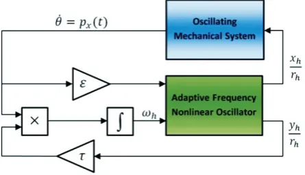
Now, we have two nonlinear dynamic systems, i.e. the mechanical stretchable pendulum and the adaptive frequency Hopf oscillator, and wish to earn an energy efficient motion pattern by exploiting the resonance mode of the mechanical system that should be found through coupling these nonlinear dynamic systems, according to the proposed learning rule, as shown in Figure 2. This coupling is established by sensory data measured from the angular velocity of the pendulum and sending it as the perturbation to the Hopf oscillator dynamics. Instead, the oscillator produces the command signals to drive the actuator. This scheme has been simulated by MATLAB/Simulink® software package, and the results are exhibited in the following. Moreover, the physical and controlling parameters used in simulation are listed in Table 1.
Solving a hybrid model, like the SP model, entails choosing a step size that satisfies both the precision constraint on the continuous state integration and the sample time hit constraint on the discrete states. The Simulink software meets this requirement by passing the next sample time hit, as determined by the discrete solver, as an additional constraint on the continuous solver. The continuous solver must choose a step size that advances the simulation up to but not beyond the time of the next sample time hit. The continuous solver can take a time step shorter than of the next sample time hit to meet its accuracy constraint but it cannot take a step beyond the next sample time hit even if its accuracy constraint allows it to.
Time evolutions of the state variables of the SP have been shown in Figure 3. We see that the steady cycles of motion appear after almost 10 seconds, which means
the controller has been able to synchronize itself with resonant mode of the mechanical system at the same duration. Approaching of the intrinsic frequency of the Hopf oscillator to a margin of the resonance frequency of the mechanical system can also be seen in the time evolution shown in Figure 4. Moreover, it is observable that the collision events have caused discontinuities (jumps) in the velocity states. The output of the Hopf oscillator that serves as the input to the actuator has also been shown in Figure 5. It is clear that after learning the resonance frequency amount of the energy required for performing the pendulum oscillations is remarkably reduced. The path emerged during the motion of the heel in X - Y plane is depicted in Figure 6. Especially, it has been marked the path is followed in the steady state.
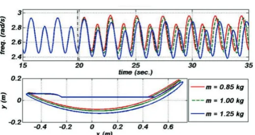
Other contribution that it is expected from the proposed controller is adaptation with probable environment changes. In order to verify this ability we re-ran our simulation code, while a sudden variation in a physical parameter considered to occur at a certain moment after the primary learning. For example, influence of changing the heel mass is seen in Figure 7. It is known that a change in the mass causes a change in the resonance frequency inversely; thus the controller tries to synchronize its intrinsic frequency with the new resonance frequency of the mechanical system, which leads to form a new pattern for motion.
Figure 2: Coupling between the mechanical system and the adaptive frequency Hopf oscillator
Table 1
The physical and controlling parameters used in simulation.
parameters m l0 k e μ ε τ γ u
Figure 3: Time evolutions of the state variables of the SP, in which the steady cycles appear after almost 10 sec
Figure 4: Time evolution of the intrinsic frequency of the Hopf oscillator
Figure 5: The output of the Hopf oscillator that serves as the input to the actuator
Figure 6: Motion path of the heel in X - Y plane
5- CONCLUSION
In this paper we presented results of coupling a nonlinear oscillator with a stretchable pendulum having a hybrid dynamic model so as to obtain energy efficient motion pattern via finding the resonance frequency given by the dynamics of the mechanical system. This idea had been originated from biological neuro - musculoskeletal system that is abundantly exploited in bio - inspired robot prototypes. Here, we employed the stretchable pendulum and the Hopf nonlinear oscillator in the role of musculoskeletal system and central pattern generator neural network, respectively. Firstly, the hybrid model of the stretchable pendulum was derived. Then, we addressed an adaptive learning rule to make a proper coupling between the mechanical system and Hopf oscillator so as to earn the energy efficient pattern. By simulating we could show that our scheme can be useful to reduce the consumed energy via adaptive pattern generating so that the mechanical system is derived near its resonant mode.
6- REFERENCES
[1] Y. Futakata, T. Iwasaki, “Entrainment to Natural Oscillations via Uncoupled Central Pattern Generators”, IEEE Trans. on Automatic Control, 56(5), pp. 1075 - 1089, 2011.
[2] S.V. Shah, S.K. Saha, J.K. Dutt, “Modular Framework for Dynamic Modeling and Analyses of Legged Robots”, Mechanism and Machine Theory, 49, pp. 234 - 255, 2012.
[3] Ph. Holmes, R. J. Full, D. Koditschek, J. Guckenheimer, “The Dynamics of Legged Locomotion: Models, Analyses, and Challenges”, SIAM Review, 48(2), pp. 207 - 304, 2006. [4] Y. Hurmuzlu, F. Geno t, B. Brogliato, “Modeling,
Stability and Control of Biped Robots — A General Framework”, Automatica, 40, pp. 1647 - 1664, 2004.
[5] I. R. Manchester, U. Mettin, F. Iida, R. Tedrake, “Stable dynamic walking over uneven terrain”, The Int. J. of Robotics Research, 30(3), pp. 265 - 279, 2011.
[6] Ch. Liu, Q. Chen, D. Wang, “CPG - Inspired Workspace Trajectory Generation and Adaptive Locomotion Control for Quadruped Robots”, IEEE Trans. on Systems, Man, and Cybernetics - Part B (Cybernetics), 41(3), pp. 867 - 880, 2011. [7] J. Rummel, Y. Blum, A. Seyfarth. “Robust and
Efficient Walking with Spring - like Legs” Bioinspiration & Biomimetics, 5(4), 046004 - 046016, 2010.
[8] J. Li, W. Chen, “Energy - Efficient Gait Generation for Biped Robot Based on the Passive Inverted Pendulum Model”, Robotica, 29(4), pp. 595 - 605, 2011.
[9] J. Nishii, T. Hioki, “Basic Concepts of the Control and Learning Mechanism of Locomotion by the Central Pattern Generator”, in: M. K. Habib (Eds.), Bioinspiration and Robotics: Walking and Climbing Robots, I - Tech Publishers, Vienna, Austria, pp. 247 - 260, 2007.
[10] Y. Futakata, T. Iwasaki, “Formal analysis of resonance entrainment by central pattern generator”, J. Mathematical Biology, 57, pp. 183 - 207, 2008.
[11] Sh. Aoi, K. Tsuchiya, “Generation of Bipedal Walking through Interactions among the Robot Dynamics, the Oscillator Dynamics, and the Environment: Stability Characteristics of a Five - Link Planar Biped Robot”, Autonomous Robots, 30, pp. 123 - 141, 2011.
[12] A. Crespi, A. Badertscher, A. Guignard, A. J. Ijspeert, “AmphiBot I: An Amphibious Snake - like Robot”, Robotics and Autonomous Systems, 50, pp. 163 - 175, 2005.
[13] J. Buchli, F. Iida, A. J. Ijspeert, “Finding Resonance: Adaptive Frequency Oscillators for Dynamic Legged Locomotion”, Proc. of IEEE/ RSJ Int. Conf. on Intelligent Robots and Systems, Beijing, China, pp. 3903 - 3909, 2006.
[14] L. Righetti, J. Buchli, A. J. Ijspeert, “Dynamic Hebbian Learning in Adaptive Frequency Oscillators” , Physica D, 216, pp. 269 - 281, 2006. [15] SMRS. Noorani, A. Ghanbari, M. A. Jafarizadeh,
![Figure 1: (a) The stretchable pendulum during its backward swinging [15]. (b) The graph of the motion sequences in a perfect cycle of the oscillations.](https://thumb-us.123doks.com/thumbv2/123dok_us/8944696.1854064/4.609.86.294.94.347/figure-stretchable-pendulum-backward-swinging-sequences-perfect-oscillations.webp)