Development of a Robust Observer for General Form Nonlinear System: Theory, Design and Implementation

Development of a Robust Observer for General

Form Nonlinear System: Theory, Design and

Implementation

B. Tarvirdizadeh

a, *

_{, A. Yousefi-Koma}

b

_{, E. Khanmirza}

c a _{Faculty of New Science and Technology, University of Tehran, Tehran, Iran, P.O. Box, 14399-57131}

b _{Faculty of Mechanical Engineering, University of Tehran, Tehran, Iran, P.O. Box, 14395-515}

c _{School of Mechanical Engineering, Iran University of Science and Technology, Tehran, Iran, P.O. Box, 16846-13114}

A R T I C L E I N F O A B S T R A C T

Article history: Received: April 28, 2015. Received in revised form: August 24, 2015. Accepted: August 29, 2015.

The problem of observer design for nonlinear systems has got great attention in the recent literature. The nonlinear observer has been a topic of interest in control theory. In this research, a modified robust sliding-mode observer (SMO) is designed to accurately estimate the state variables of nonlinear systems in the presence of disturbances and model uncertainties. The observer has a simple structure but is capable of efficient observation in the state estimation of dynamic systems. Stability of the developed observer and its convergence is proven. It is shown that the estimated states converge to the actual states in a finite time. The performance of the nonlinear observer is investigated by examining its capability in estimation of the motion of a two link rigid-flexible manipulator. The observation process of this system is complicated because of the high frequency vibration of the flexible link. Simulation results demonstrate the ability of the observer in accurately estimating the state variables of the system in the presence of structured uncertainties along with different initial conditions between the observer and the plant.

K e y w o r d s : Nonlinear observer Sliding mode observer State estimator Robotic manipulator Dynamic modelling

1. Introduction

State space control techniques rely on the availability of all state variables of the system for the computation of control actions. However, in many situations, the number of the state variables exceeds that of the measured signals. This may be due to the cost associated with additional sensors, the lack of appropriate space to mount transducers, or the hostile environment in which the sensors must be located. In these conditions, either a full-order or a reduced-order observer can

* _{Corresponding address: Faculty of New Science and Technology, University of Tehran, Tehran, Iran,}

Tel.: +98 2161115775; fax: +982188497324, E-mail address: [email protected]

be implemented to estimate the state variables from the inputs and the measured outputs of the system [1]. Observer design is crucial to the identification and control problems [1, 2].

nonlinear observers with linearizable error dynamics can be designed. Some observers were designed for a restricted class of nonlinear systems such as bilinear systems [7, 8]. A novel SMO for current-based sensor less speed control of induction motors is presented in [9].

Sliding mode control is a popular control approach for systems containing uncertainties or unknown disturbances, as the controllers can be designed to compensate for such uncertainties or disturbances. Similar to sliding mode controller (SMC), sliding mode observers include a special function of dealing with nonlinearity and uncertainties. Over the past decades, extensive research has been dedicated to the design of SMOs [10-12].

A very important feature of the SMC stems from the fact that the attractive manifold is an invariant set ([13, 14, 27]). When the controlled system is in the sliding mode, its response becomes insensitive to external disturbances and model uncertainties. Such salient features have rendered the SMC a potential tool for achieving robust tracking performance for robotic manipulators in the presence of structured and unstructured uncertainties along with external disturbances [15]. Walcott and Zak [16] developed a variable structure observer for systems with observable linear parts and bounded nonlinearities and/or uncertainties. Wagner and Shoureshi [17] compared the performances of three nonlinear observers in estimating the state variables of a heat exchanger [18, 19]. Slotine et al. [11] proposed SMOs for general nonlinear systems. They discussed in detail the design procedure of variable structure system (VSS) observers for the nonlinear systems expressed in the companion form. Roopaei [20] developed a novel Adaptive Fuzzy Sliding-Mode Control methodology, based on the integration of SMC and Adaptive Fuzzy Control. Shkolnikov et al. [21] demonstrated the application of a second-order SMO. Imine et al. [22] proposed a SMO for systems with unknown inputs. The system considered was a vehicle model with unknown inputs that represent the road profile variations. Kalsi et al. [23] designed a SMO for linear systems with unknown inputs, where the observer matching condition was not satisfied. Efimov and Fridman [24] proposed a state observer design procedure (SMO with adjusted gains) for nonlinear locally Lipschitz systems with high relative degree from the available for measurements output to the nonlinearity. Possible presence of signal uncertainties had been taken into account. Veluvolu and Lee [25] developed a robust high-gain observer for state and unknown

input estimations in a special class of single-output nonlinear systems. They showed, ensuring the observability of the unknown input with respect to the output, the disturbance could be estimated from the sliding surface.

The purpose of the current study is to develop a new type of robust nonlinear SMO to estimate the state variables of nonlinear systems in the presence of structured uncertainty and different initial conditions between the observer and the plant. Stability of the estimated states as well as their finite time convergence to the actual states have also been proven. The estimator consists of a VSS observer with a structure similar to that of the one proposed by Slotine et al. [11] for general nonlinear systems.

2. Problem formulation

In this section, a robust sliding-mode observer is introduced for nonlinear systems. In the next sections, we will generalize this observer and will develop a new form of SMO, while stability and convergence analysis will be carried out.

Consider an nth-order nonlinear system as: (1)

   

n

R t f xu x x , ,

The state vector

x

is defined as x



x₁  x_n



T, where xiR. In this study

m R



u is considered as the control input. A vector of measurements is defined in the following form:

(2) 1 2

T p

m m mp

x x x R

 

_{ } 

Y Y

It means that the state variables

mp m

m x x

x ₁, ₂,, are available through measurement, directly. Matrix C could be introduced in the following form:

(3)

n mp mp

m m



    

 

    

 

 

0 0 1 0 0

0 0 1 0 0

0 0 1 0 0

, 2

1

 

       

 

 

C Cx Y

All elements of every row of C are equal to zero except for the mkth elements, which equal to unity. These elements correspond to the kth

measured state (x_mk, k1,2,,p). By this definition, the error vector could be formulated as



x x



x x x

C Y Y

e: ˆ  ˆ ~:ˆ (4) where xˆRn is the estimated state vector, and

(5)





T

p e e e

e1 2 3 

: e

The following assumptions are made for the plant and the input vector;

Assumption 2. f

 

x,u is bounded away from zero for

n

R



x and t0.

Assumption 3. Every control input u_i ( i1,,m) belongs to the extended L_p space denoted as L_pe. Thus,

any truncation of u_ito a finite-time interval is essentially bounded.

Assumption 4. The unknown disturbance input is bounded by some known upper bounds.

Hence, an observer with the following general structure is defined [11]:

(6)

 

xu Pe Q1s

f

xˆˆˆ,  

where fˆis an approximate model of f , while P and Q

are npgain matrices to be defined, and 1_s is a p1 vector specified as follows:

 

 

 

 





T

p e e

e

e sgn sgn sgn

sgn 1 2 3 



s

1 (7)

3. Stability and Convergence Analysis

In this section, it will be shown that the estimated states converge to the actual plant states in a finite time interval. In order to prove the finite-time convergence of the estimated state to the actual one, the Comparison Lemma is used [26].

Lemma 1. (Comparison Lemma). Consider the scalar differential equation,

 

z,t, z

 

t0 z0

g

z 



where g

 

z,t is continuous in t and locally Lipschitz in z for t0and zJR. Let



t0,T



(T could be

infinity) be the maximal interval of existence of the solution z

 

t , and suppose z

 

t J for all t



t0,T



.

Let v

 

t be a continuous function whose upper right-hand derivative Dv

 

t satisfies the differential inequality

 

t g



v

 

t,t



, v

 

t0 z0 v

D  

with v

 

t Jfor all t



t0,T



_{. Then} v

   

t zt _{is true for} all t



t0,T



_.

In the following theorem, the stability and convergence of the SMO in the presence of structural uncertainty in the system dynamics, is proven.

Theorem 1. Consider the plant of equation (1), the measurements vector (2), the observer (6), and the assumptions 1-4. Then, there exist observer gain matrices, Pand Q, such that the estimated state

x

ˆ

converges to the actual state x in a finite time.

Proof. A general form of plant and observer is considered in this study. At the beginning of the

observation process, the observation error is far away from zero, which means that e0. We define a Lyapunov function for all the measured states (x_m1,x_m2,,x_mp). In this theorem, the stability and convergence time of the observer has been shown for an arbitrary measured state (which is also easy to be applied to other measured states). Consider a measured state x_mj,

where j is an element of the set



1,2,,p



. The following candidate for the Lyapunov function is defined for this state (x_mj):

(8) 2 5 . 0 j j e

V  

Consequently

 

 

_     _{  }               









    mp m i i mi j mp m i i mi j j j mp m i i mi j mp m i i mi j j j j j j j e p e q f e e p e q f f e e e V 1 , 1 , 1 , 1 , sgn sgn ˆ   (9)

where f_j fˆ_jf_j. Moreover, fˆ_j and f_j represent the jth row of the system dynamics

vectors fˆ and f in the measured space domain, respectively. Note that according to the assumptions 1-4, f_j is bounded. The 3rd _{term of} the above equation is rewritten as follows;

(10)

 

 

 

 

 

 

jj

 

j mp mj i m i i mi j p mp j j mj j m j m j mp m i k mi j e q e q e q e q e q e q i q sgn sgn sgn sgn sgn sgn sgn , 1 , , , 2 2 , 1 1 , 1 ,        





    

Assuming P0 (for simplicity), substituting equation (10) into (9) results in the following:

(11)

 

 

 

 

 

j j j j j j j j j j j j j j j j j j j j mp mj i m i i mi j j j j j j j mp mj i m i i i j j j j e q E e q e E e e q e E e e q e e q e f e e q e q f e V                                    





    , , , , 1 , , 1 , sgn sgn sgn sgn sgn 

where



 

      mp mj i m i i mi j j

j f q e

E

1

, sgn . Thus:



jj j



j j j j j j

j e E q e e q E

Choosing q_j,_j E_j _j where j 0

yields V_je_j _j which, in turn, ensures that

0



j

V for all e_j 0, as well as ensures the finite time convergence of e_j to the zero. In order to prove that the convergence happens in a finite time interval, function G_j is defined as

j j

j V e

G  2  . As a result:

(13)



j j



j

j j j

j j j j

e e V e

V V G G D

      

 



1 1

2 1



 

Subsequently, DG_j



_j. Let us define

 

j j j G t

g ,  then DG_jg

 

G_j,t . Now, consideringz_jg_j

 

z,t _j,zj

 

t₀ Gj

 

ej

 

t₀

yields the following:

(14)

 

 





 

 

0



0



0 0

0 0

t t t

z t z

t t t

z t z

d d

d dz

j j j

j j

j

t

t j t

t j

   

     

 



_



 

   

Applying Lemma 1, G_j

 

t g_j

 

t . Thus,

(15)

 

t G



e

 

t0





t t0



Gj  j j j 

Since G_je_j , it is clear from above equations that there will be a finite time period during which

j

e reaches zero. In order to prove for the upper

bound of the time interval, set

 



e t0





t t0



G_{j j} _j  . Accordingly, by the time

 

0 0

: e t t

T t

j j

j  

 _ , the state e_j converges to the

zero.

It is shown that for any measured state, the observation error (in the estimation of the measured state) will converge to zero in a finite time. Applying q_j,_j E_j _j for any

measured state, forces the system to satisfy e0

in the presence of model imprecision, disturbances and structural uncertainties.

Heretofore, stability and finite time convergence of the measured state variables to the actual state variables were proven. Now we want to study the convergence of the unmeasured state variables to the actual state variables.

The complement of e is defined as e, where e is p dimensional and e is n-p dimensional. e

is estimation error of unmeasured state variables. These two error vectors can be arranged as follow









    

1 1 1 2 1 2 2 1 2 2

e f e ,e v e f e ,e v u (16) where e1e is p dimensional and e2e is n-p dimensional. v₁ and v₂ are the noise and/or uncertainty terms, and u is the estimational correction term. An appropriate sliding surface is defined as S0, where

(17)

 

1 2 ge

e S 

The function g

 

e₁ is to be determined in such a way that the differential equation obtained as

(18)

 

1 1 1



1

 

1



1 1

1 h e v f e , ge v

e     

describes an asymptotically stable system. In other words, when the error state happens to be on the surface S0, v₁ is sufficiently suppressed and e₁ slides down to zero. Of course, g

 

e₁

must also be such that g

 

0 0. Thus, when

0



S , i.e. when e₂ g

 

e₁ , as e₁ slides down to zero, it also drags e₂ to zero alongside with itself. Consequently, both e₁ and e₂ become zero and thus the whole state vector (x) of the system will have been estimated. On the other hand, the error state can be attracted to the sliding surface and kept on it by stipulating the following condition:

(19) 0

 S ST 

Here, ST denotes the transpose of S. By substituting the preceding equations, this condition can be written as

(20)





 





   









  



 

0

0

 

_    _

 

    

 

 _{ }



 

 

   

 _ _

  

 

1 T

2 1 2 2 1

1

2 1 2 2

T 1

1 1 2 1

1

2 1 2 1 1 2

T

2 1

dg e

S f e ,e v u e

de

f e ,e v u S dg e

f e ,e v de

f e ,e G e1 f e ,e S

v u G e1 v or more compactly as

(21)







 



0

f e ,e v u S 21 1 2 21

T

As far as v₂₁ is concerned, the worst case occurs if

(22)

 

S sgn V v21 

where, Vmax



mag

 

v₂₁



and

 

sgn

 

1 sgn

 

2

T

s s etc

 _ _

sgn S . With this worst

(23)



e ,e



u V sgn

 

S C S f21 1 2     1

Here, C₁ is a positive definite matrix. Hence, the estimational correction term is determined as

(24)





 



f e ,e V sgnS C S



u _{21 1 2}    ₁ and the proof completes.■

So far, the structure of the nonlinear SMO has been defined and its convergence time and stability have been proven. In the next section, some additional changes are introduced in the observer structure to increase its performance.

4. Observer Development and Generalization

In the previous section, the convergence of the estimated state to the actual plant state in a finite time period has been proven. In this section, a generalized form of the observer introduced in equation (6) has been developed in two steps.

Step 1: In order to alleviate unacceptable errors whenever the actual and estimated state vectors have different initial conditions, a feedback loop based on the estimated state variables is introduced to modify the observer structure.

Equations (1) and (2), define plant and measurements vectors. Let us put forth the following notation:

(25) p

R



 m

m Y x

x ,

m

x represents the corresponding vector of measured states, where

m





m

1

,

m

2

,



,

mp



and

m

x is defined as, x_m



x_m1,x_m2,,x_mp



. The unmeasured states (to be estimated by the observer) are evaluated as follows:

(26)



x1,x2,,xn







xm1,xm2 ,,xmp





um x

The observer structure can then be written as:

(27)

 

 

s

s

1 Q e P u x f x

1 Q e P u x f x

um um um um

um

m m m m

m

  

  

, ˆ ˆ

, ˆ ˆ

 

The derivation of fˆm

 

x,u and fˆum

 

x,u is based

on xˆ_m and xˆ_um (equations (25) and (26)), respectively. Matrices Pm and Qm are of the size

mp

mp , while matrices P_um and Q_um are



nmp



mp, whereas vectors 1_ms and 1_ums have mp and (n-mp) elements, correspondingly. Now, it is the time of applying the first step modification on the observer structure as follows:

 

 

um um um um

um um

m m m m

m

K x

1 Q e P u x f x

1 Q e P u x f x

s s

ˆ ,

ˆ ˆ

, ˆ ˆ

  

 

  

 

(28)

where K is a diagonal matrix with (n-mp) elements. K may be selected so as to provide eigenvalues with negative real components for the homogeneous terms of the corresponding equations of xˆ_um. Equation (28) consists of two parts; namely estimation of the measured states and estimation of the unmeasured ones. The second change in the observer structure to improve the estimation performance and robustness is introduced in the following step.

Step 2: In this step, another term is added to the previous structure of the observer as follows:

 

 

_



    

 

  

 

t

t um um um

um um um

um

t

t m m m m m

m

K

0 0

ˆ ,

ˆ ˆ

, ˆ ˆ

edt K x 1

Q e P u x f x

edt K 1 Q e P u x f x

s s

 

(29)

where K_m is a square matrix with mp rows, K_um

is a matrix with (n-mp) rows and mp columns,

and

T t

t mp t

t t

t t

t

e e e

    

  



_

_

_



0 0 0 0

2

1 

e represents a vector

containing the integral of errors in the estimation of the measured states. As seen, the integral of errors is taken into account in the estimation process. This is the final form of the developed nonlinear sliding-mode observer in this study. The developed observer accurately estimates the unknown states, in a finite time interval, and in the presence of structured uncertainties, while the observer and the plant have been under different initial conditions.

There is no need to any further proof for validity of Theorem 1 for developed observer in equation (29) because all added terms in equation (29) with respect to equation (6)- could be included in functions f1



e1,e2



and f2



e1,e2



of equation (16). The observer developed here has been tested on various nonlinear systems for which all simulations have confirmed its performance in estimation of the states of the nonlinear systems. In the next section, the performance of this observer on the state estimation of a nonlinear system consisting of a rotating two link rigid-flexible manipulator is demonstrated.

5. Implementation of the Developed Nonlinear Observer

assumed modes method is implemented to approximate y

 

x,t (flexural deformation of the link) which is considered here to be dominated by the first three elastic modes. y

 

x,t is a linear combination of shape functions 

 

x , of spatial coordinates i

 

x , and time-dependent

generalized coordinates qbi

 

t . Thus [27]:

(30)

 

,

   

, ₁ 3

1 1   

_

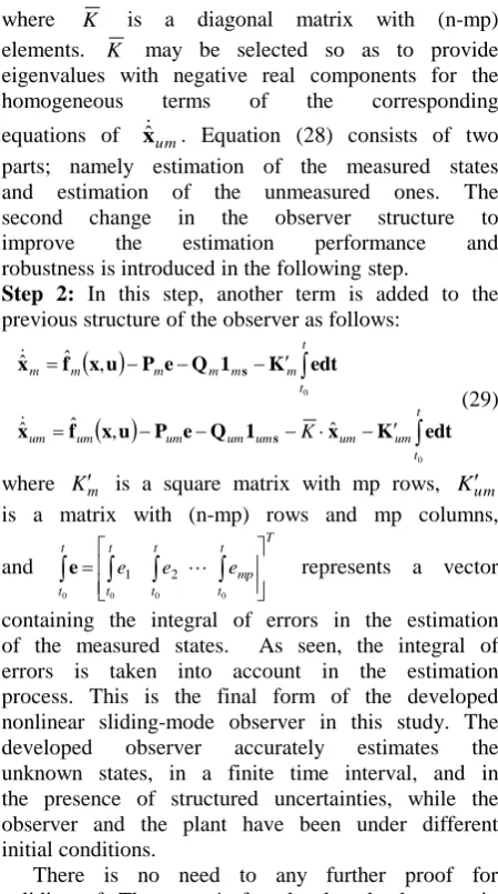
 n t q x t x y n i bi i 

Consider two frames of references: x₁y₁

and x₂y₂, are fixed to the rigid bases and rotate with angular velocities ₁ and ₁₂, respectively. Second Link (Flexible) First Motor Second Motor 1  2  First Link

(Rigid) 1

Y

X

2 2Oh

1 x 1

y

2

x

2 y 2  1

2Oh

Payload

Figure 1: Schematic of the two link rigid-flexible manipulator

The velocity vector of an infinitesimal mass element on the flexible link and flexible link tip are given as follows:





 

 

 





 

 

  



 

 

 

 

 

 

 

   



2 2 2 2 1 1



1

1 2 2 2 2 1 1 1 1 1 2 2 2 2 2 1 2 2 2 2 2 sin cos cos sin cos sin sin cos cos sin cos sin j L Y Y L i Y Y L j O l O y y x O i y y x O a a a a t h h h                                                                                     t2 2 V V (31)

where



 

 



T i1 cos1 sin1 

,



 

 



T j1 sin1 cos1 

,

 

x t y

y 2, ,Yy

 

l2,t , y



x t



t

y _ 2,

 

 , y

 

l t

t

Y _ 2,

 

 _,

 

l t O y

 

l t y

Y_a ₂,  _t2  ₂, ,L₁l₁O_h1O_t1, 2

2 2

2 l Oh Ot

L    and 12.

The total kinetic energy of the system is:

(32)

























2

2 2 2 2 1 2 1 2 2 2 2 1 2 1 1 2 1 1 2 2 0 2 2 2 1 1 1 0 1 2 1 1 1 1 , 2 1 2 1 2 1 2 1 2 1 2 1 2 1 2 1 2 1 t l x y I L m I L m I m dx m I dx x O m E t h h t t t l l h l h l kin                





               t2 t2 2

2 V V V

V

The potential energy of the system is given by:

(33)









2 0 2 2 2 2 2 2 2 _, 2 1 dx x t x y EI E l

pot





        

where, l1.31mis length of the link,

m kg

ml 1.179 / is mass per unit length of the

link, E = 206GPa is Young’s modulus of elasticity, mt0.4kg is tip mass, mh0.3kg is

mass of hub, I0.3797109m4 is area moment of inertia of the cross-section area of the link about the rotating axis, I_t0.0139kg.m2 is tip-mass moment of inertia about its CG axis, and

2 . 142 .

0 kgm

I_h is hub mass moment of inertia about the rotating axis. The variation of the nonconservative work is:

(34) 2

2 1 1  

 W 

where ₁ , ₂ are torques applied by the first and second motors, respectively.

System Lagrangian is defined as:

(35) pot kin E E   

The detailed expression of  will be available, if it is needed. The equation of motion is then obtained by: (36) m j q W q q dt d j j j , , 2 , 1 ,     _                        

In our formulation, we have:

(37)

  , 5 , , , , , 2 2 4 1 3 2 2 1 1        m q q q q q q q q m b m b b   

The equations governing the rigid and flexible motions of the manipulator consist of five nonlinear, coupled, stiff, second-order ordinary differential equations. These equations are then converted to a set of 10 first-order ordinary differential equations, which are given as:

(38)

 

 

 

xu

 

xu

 

xu

u x u x , , , , , , , , , , , , , 10 10 9 9 8 8 7 7 6 6 10 5 9 4 8 3 7 2 6 1 f x f x f x f x f x x x x x x x x x x x                    



1 2 3 4 5 6 7 8 9 10



1 2 1 2 3 1 2 1 2 3

T

T

b b b b b b

x x x x x x x x x x

q q q q q q

          x (39)

Equations (38) and (39) are the state space representation of the system. There is no analytical solution for these state equations, thus they are solved numerically in this study.

Nonlinear Observer Design

In this part the designed observer in the previous sections will be implemented on the above nonlinear system. The objective of the robust nonlinear observer is to estimate q1_b, q2b,

b

q3 , q1b, q2band q3b, in the presence of

disturbances and model uncertainties. In designing the observer,



1,



2, 1 and 2 are assumed to be known from measurements.

According to equations (1), (2) we have: n=10, p=4, x_m1₁, x_m2₂, x_m3₁,

2 4 

m

x and there are also, (n-p)=6 unmeasured state variables which we define as

x

_um1



q

_b1,

2

2 b

um

q

x



,

x

_um3



q

_b3,

x

_um4



q



_b1,

x

_um5



q



_b2

and

x

um6



q



b3. Note that



x_m1 x_m2 x_mp







x_um1 x_um2 x_um_np





 

X . The assumptions which had been mentioned in this paper are satisfied in the system given by equation (38).

An observer with an initial structure similar to equation (6) (without generalization in this step) is defined as follow:

(40)

 

x Pe Q1s

f

xˆˆˆ,t  

According to the previous explanation, for the manipulator system studied in this paper C is given as follows:

(41) 1 1 2 2 6 3 7 4

1 0 0 0 0 0 0 0 0 0

0 1 0 0 0 0 0 0 0 0

0 0 0 0 0 1 0 0 0 0

0 0 0 0 0 0 1 0 0 0

x y x y C x y x y                   _{ }_{ }_{ }             Consequently:









T T x x x x x x x x     _{   }         2 2 1 1 2 2 1 1 7 7 6 6 2 2 1 1 ˆ ˆ ˆ ˆ ˆ ˆ ˆ ˆ ˆ             x x C e (42)

By adopting the observer structure developed previously, the state equations of the estimator can be written as (without modification of the observer structure in this step):





 

 

 

 





 

 

 

 

1 6 11 1 12 2 13 6 14 7

11 1 12 2

13 6 14 7

2 7 21 1 22 2 23 6 24 7

21 1 22 2

23 6 24 7

9 9 91 1 92 2

93 6 94 7

ˆ

ˆ

(

sgn

sgn

sgn

sgn

)

ˆ

ˆ

sgn

sgn

sgn

sgn

ˆ

ˆ

{

x

x

P x

P x

P x

P x

Q

x

Q

x

Q

x

Q

x

x

x

P x

P x

P x

P x

Q

x

Q

x

Q

x

Q

x

x

f

P x

P x

P x

P x































































 

 

 

 

 

 

 

 

91 1 92 2

93 6 94 7

10 10 101 1 102 2

103 6 104 7

101 1 102 2

103 6 104 7

}

{

sgn

sgn

sgn

sgn

}

ˆ

ˆ

{

}

{

sgn

sgn

sgn

sgn

}

Q

x

Q

x

Q

x

Q

x

x

f

P x

P x

P x

P x

Q

x

Q

x

Q

x

Q

x











































(43)

P represents the Luenberger observer gain matrix determined based on the A and C

matrices obtained by linearization of equation (38) around xˆ0. In this study P is obtained by assigning i5 i1,2,,10 as the desired

eigenvalues of



APC



. It should be noted that

7 , 6 , 2 , 1 ~_{x i}

P i provides additional corrective

action that helps the system in reaching the sliding surface.

For simplicity, the above equations are shown as: 10 , 2 , 1 , ˆ 

 _{F i}

xi i (44)

The preliminary results have demonstrated that the above observer suffers from unacceptable errors whenever the actual and estimated state vectors have different initial conditions. In order to alleviate this problem, equations (43) are modified by introducing a feedback system based on the estimated state variables as follows (applying first step observer structure modification in this paper):

10 10 10 10 9 9 9 9 8 8 8 8 7 7 6 6 5 5 5 5 4 4 4 4 3 3 3 3 2 2 1 1 ˆ ˆ , ˆ ˆ , ˆ ˆ , ˆ , ˆ ˆ ˆ , ˆ ˆ , ˆ ˆ , ˆ , ˆ x K F x x K F x x K F x F x F x x K F x x K F x x K F x F x F x                           (45)

parts for the homogeneous parts of the corresponding equations of xˆ3,xˆ4,xˆ5,xˆ8,xˆ9,xˆ10. Note that in this system:

1 1 2 2 3 6 4 7

1 3 2 4 3 5 4 8

5 9 6 10

, , ,

, , , ,

,

m m m m

um um um um

um um

x x x x x x x x

x x x x x x x x

x x x x

   

   

 

(46)

Equations (43), (44) and (45) represent the nonlinear designed observer. This structure has then been changed with the application of the 2nd step modification of the observer structure (developed in equation (29)) to increase the observation performance. The new observer structure has been developed with respect to equations (45) with consideration of integral of error in the observation process, the observer structure is represented in the following form:

1 1 1 2 2 2 3 3 3 3 3

4 4 4 4 4 5 5 5 5 5

6 6 6 7 7 7 8 8 8 8 8

9 9 9 9 9 10 10 10 10 10

ˆ , ˆ ,ˆ ˆ ,

ˆ ˆ ˆ, ˆ

ˆ ,ˆ , ˆ ˆ ,

ˆ ˆ , ˆ ˆ

x F IE x F IE x F IE K x

x F IE K x x F IE K x

x F IE x F IE x F IE K x

x F IE K x x F IE K x

      

     

      

     

(47)

where

. ~ ~

~ ~

0 7 4 0 6 3 0 2 2 0 1

1



 



 



 





 t

i t

i t

i t

i

i K xdt K x dt K x dt K x dt

IE

This is the final form of the developed observer for the two link rigid-flexible manipulator. This observer can accurately estimate unknown states, in the presence of structured uncertainties and under different initial conditions between the observer and the plant.

With a simple but understandable structure and accurate estimation of state variables this has some benefits over nonlinear observer, such as adaptive-gain observer that ensures its application in nonlinear systems.

6. Results

The designed observer was tested for various initial conditions and structural uncertainties, some of which are presented in this paper. For the two link rigid-flexible manipulator used in this study, the inputs are i,i1, 2, representing the first and the second electric motor torques, respectively. The state vector is





T

b b b b

b

b q q q q q

q1 2 3 1 2 1 2 3

2

1      



 x

in which



₁,



₂, ₁ and ₂are derived from measurements, directly. The objective of the robust nonlinear observer is to estimate q1_b, q2b,

b

q3 , q1b, q2b and q3b accurately, in the

presence of model uncertainties and under different initial conditions between the observer and the plant.

The following disturbances are considered in the observer model:

1- 12.5% difference in the mass of end effector between the observer model and the plant model (see appendix for the lagrangian of the actual and disturbed system).

2- 9 degree difference in the initial condition of second motor angle.

It is important to mention that the disturbed end effector mass not only changes the system model but also the mode shapes of the flexible link and consequently the overall system will be disturbed.

The applied torques by electric motors are shown in Figure2. The dashed line shows the torque of first motor, and the solid one represents the second motor torque. The flexible link tip displacement in the rotating frame, x₂y₂, is presented in Figure3. As seen, that the flexible link has a tip displacement in the range of about 7mm. Tip vibration of the flexible link is shown in Figure3.

Angular displacements of the first and second motors are shown in Figure4 and Figure5 , respectively. Although states



₁,



₂, ₁ and ₂ are derived from measurements, they are estimated by the observer as well, to determine the observation error in these variables. This error is employed for estimation of state variables, q1_b,

b

q2 , q3b, q1b, q2band q3b. The first motor has

stats, and have to be estimated by the designed observer. States x3q1_b, x4q2b and x5q3b

have strong vibrations with very small amplitude, which complicate the observation process. However, results showed that the designed observer had estimated states accurately.

The angular velocities of the first and second motor are illustrated in Figure 12 and Figure 13, respectively. ₁ and ₂ are the measured states.

1

 _and

2

 _{are also estimated (in addition to}

measurement), to evaluate the observation error in these variables. The maximum angular velocities

of the first and the second motor are 25 deg/sec and -70deg/sec, respectively (Figure 12 and Figure 13). The convergence of the observer output to the plant output in the estimating q1b is illustrated in

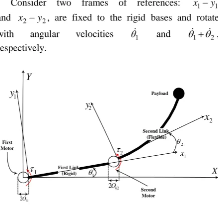
Figure 14. Time derivative of the second elastic mode of the flexible link is demonstrated in Figure 15 and Figure 16, which illustrate the convergence of the observer output to the plant output precisely. Similarly, time derivative of the third elastic mode of the flexible link are shown in Figure 17 and Error! Reference source not found..

Figure2: Applied torque by motors Figure3:Tip displacement of the flexible link

Figure4: Angular position of the first motor Figure5: Angular position of the second motor

Figure 6: Magnification of Figure5 at the beginning of

observation Figure 7: First elastic mode of the flexible link

Figure 8: Second elastic mode of the flexible link Figure 9: Magnification of Figure 8 at the beginning of _observation

0 1 2 3 4

-2 -1 0 1 2 3

Motors Torque

t (sec)



(N

.m

)

First Motor Second Motor

0 1 2 3 4

-0.01 -0.005 0 0.005 0.01

Tip Displacement of the Flexible Link

t (sec)

y

(x2

=L

2

,t)

(m

)

0 1 2 3 4

-10 0 10 20 30 40

x

1

t (sec)

1

(deg

)

Actual Estimated

0 1 2 3 4

-150 -100 -50 0

x

2

t (sec)

2

(deg

)

Actual Estimated

0 0.05 0.1 0.15 -10

-8 -6 -4 -2 0

x₂

t (sec)

2

(deg

)

Actual Estimated

0 1 2 3 4

-0.01 -0.005 0 0.005 0.01

x

3

t (sec)

qb

1

Actual Estimated

0 1 2 3 4

-4 -2 0 2 4x 10

-4 x4

t (sec)

qb

2

Actual Estimated

0 0.5 1 1.5

-2 -1 0 1

x 10-4 x4

t (sec)

qb

2

Figure 10: Third elastic mode of the flexible link Figure 11: Magnification of Figure 10 at the beginning of simulation

Figure 12: Angular velocity of the first motor Figure 13: Angular velocity of the second motor

Figure 14: Time derivative of the first elastic mode of the

flexible link Figure 15: Time derivative of the second elastic mode of the flexible link

With respect to these results, it is seen that the observer accurately estimates unmeasured states in the presence of unstructured uncertainties, and

difference of initial condition between the plant and observer accurately.

Figure 16: Magnification of Figure 15 at the beginning of observation

Figure 17: Time derivative of the third elastic mode of the flexible link

0 1 2 3 4

-1 -0.5 0 0.5

1x 10

-5 x5

t (sec) q b

3

Actual Estimated

0 0.5 1 1.5

-5 0 5

x 10-6 x5

t (sec)

qb

3

Actual Estimated

0 1 2 3 4

-10 0 10 20 30

x₆

t (sec)

d

1

/dt

(deg

/s

ec)

Actual Estimated

0 1 2 3 4

-80 -60 -40 -20 0 20

x

7

t (sec) d

2

/dt

(deg

/s

ec)

Actual Estimated

0 1 2 3 4

-0.1 -0.05 0 0.05 0.1

x

8

t (sec)

d(q

b

1

)/

dt

Actual Estimated

0 1 2 3 4

-0.02 -0.01 0 0.01 0.02

x

9

t (sec)

d(q

b

2

)/

dt

Actual Estimated

0 0.2 0.4 0.6

-0.01 -0.005 0 0.005 0.01 0.015

x

9

t (sec)

d(q

b

2

)/

dt

Actual Estimated

0 1 2 3 4

-2 0 2 4 6x 10

-4 x10

t (sec)

d(q

b

3

)/

dt

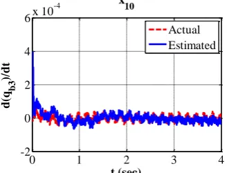
Figure 18: Magnification of Figure 17 at the beginning of observation

7. Conclusion

In this study, a novel nonlinear sliding-mode observer (SMO) was designed for a general form of nonlinear systems. Stability of the observer as well as a finite time convergence of the designed observer were also been proven. The SMOs turned out to have intriguing properties in the presence of disturbances, and tended to demonstrate predictability robustness properties in the presence of model uncertainties. The integral of errors occurred in the observation process was employed to develop the observer structure. This simple structure is very convenient to use in other nonlinear systems. The developed SMO is able to provide appropriate estimation of the unmeasured state variables in the presence of unstructured uncertainty. The designed observer, in this paper, was utilized in a two link rigid-flexible manipulator to demonstrate observer ability and performance in state observation. Using Lagrange principle a mathematical model of the two link rigid-flexible manipulator was developed. The assumed modes method was used for modelling the transverse deflection, which was considered to be dominated by the first three elastic modes. The observation process of this system was complicated due to the high frequency vibration of the flexible link and rapid changes in states. The rigid and flexible links behavior was estimated by the measurement of angular position and velocity of motors. The position and velocity of the links and consequently, end effector were then estimated. Results illustrated the ability of the observer, with a simple structure, in accurately estimating the state variables of the rigid-flexible manipulator in the presence of structured uncertainties and different initial conditions of the plant and observer states.

References

[1] N. G. Chalhoub, G. A. Kfoury, Development of a robust nonlinear observer for a single-link flexible manipulator, Nonlinear Dynamics, Vol. 39(3), (2005), 217-233.

[2] G. Besancon, Nonlinear observers and applications”, springer, 2007.

[3] T. A. Ahmed, G. Kenne, F. L. Lagarrigue, Identification of nonlinear systems with time-varying parameters using a sliding-neural network observer, Neurocomputing, Vol. 72(7-9), (2009), 1611–1620.

[4] S. Ibrir, On observer design for nonlinear systems, International Journal of Systems Science, Vol. 37(15), (2006), 1097–1109.

[5] C. Califano, S. Monaco, D. Normand-Cyrot, Canonical observer forms for multi-output systems up to coordinate and output transformations in discrete time, Automatica Vol. 45(11), (2009), 2483–2490.

[6] D. Bestle, M. Zeitz, Canonical form observer design for nonlinear time-variable systems, International Journal of Control Vol. 38(2), (1983), 419–431.

[7] J. P. Gauthier, I. Kupka, A separation principle for bilinear systems with dissipative drift, IEEE Transactions on Automatic Control, Vol. 37(12), (1992), 1970–1974.

[8] G. Bornard, N. Couenne, F. Celle, Regularly persistent observers for bilinear systems, New Trends in Nonlinear Control Theory, Vol. 122, (1989), 130–140.

[9] A. J. Krener, A. Isidori, Linearization by output injection and nonlinear observers, Systems & Control Letters, Vol. 3(1), (1983), 47–52.

[10] C. Aurora, A. Ferrara, A sliding mode observer for sensorless induction motor speed regulation, International Journal of Systems Science, Vol. 38(11), (2007), 913–929.

[11] J. J. E. Slotine, J. K. Hedrick E. A. Misawa, On Sliding mode observers for nonlinear systems, Journal of Dynamic Systems, Measurement, and Control, Vol. 109, (1987), 245–252.

[12] A. Koshkouei, A. Zinober, Sliding mode state observation for non-linear system, International Journal of Control, Vol. 77(2), (2004), 118-127.

[13] J. Ahrens, H. Khalil, High-gain observers in the presence of measurement noise: a switched-gain approach, Automatica, Vol. 45(4), (2009), 936-943.

[14] J. J. E. Slotine, W. Li, Applied Non-linear Control, Prentice-Hall, Englewood Cliffs, NJ, 1991.

[15] H. Lee, E. Kim, H. J. Kang, M. Park, A new sliding-mode control with fuzzy boundary layer, Fuzzy Sets and Systems, Vol. 120, (2001), 135– 143.

[16] G. Bartolini, E. Punta, T. Zolezzi, Simplex sliding mode methods for the chattering reduction

0 0.1 0.2 0.3 0.4

0 1 2 3 4x 10

-4 x10

t (sec)

d(q

b

3

)/

dt

control of multi-input nonlinear uncertain system, Automatica, Vol. 45(8), (2009), 1923-1928.

[17] B. L. Walcott, S. H. Zak, Observation of dynamical systems in the presence of bounded nonlinearities/uncertainties, Proceedings of the 25th _{IEEE Conference on Decision and Control,} Athens, Greece, (1986), 961–966.

[18] J. Wagner, R. Shoureshi, Observer designs for diagnostics of nonlinear processes and systems, Proceedings of the ASME WAM, Dynamic Systems and Control Division, WA/DSC-5, Chicago, IL, (1988).

[19] F. E. Thau, Observing the state of non-linear dynamic systems, International Journal of Control, Vol. 17(3), (1973), 471–479.

[20] W. Baumann, W. Rugh, Feedback control of non-linear systems by extended linearization, IEEE Transactions on Automatic Control, Vol. 31(1), (1986), 40–47.

[21] M. Roopaei, M. Zolghadri, S. Meshksar, Enhanced adaptive fuzzy sliding mode control for uncertain nonlinear systems, Communications in Nonlinear Science and Numerical Simulation, Vol. 14(9-10), (2009), 3670-3681.

[22] I. A. Shkolnikov, Y. B. Shtessel, D. P. Lianos, Effect of sliding mode observers in the homing guidance loop, Proceedings of the Institution of Mechanical Engineers, Part G: Journal of Aerospace Engineering Vol. 219 (2), (2005), 103-111.

[23] H. Imine, N. K. M’Sirdi, Y. Delanne, Sliding-mode observers for systems with unknown inputs: application to estimating the road profile, Proceedings of the Institution of Mechanical Engineers, Part D: Journal of Automobile Engineering, Vol. 219(8), (2005) 989-997.

[24] K. Kalsi, J. Lian, S. Hui, S. H. Zak, Sliding-mode observers for systems with unknown inputs: A high-gain Approach, Automatica, Vol. 46(2), (2010), 347-353.

[25] D. Efimov, L. Fridman, Global sliding-mode observer with adjusted gains for locally Lipschitz systems, Automatica, Vol. 47(3), (2011), 565– 570.

[26] K. C. Veluvolu, D. Lee, Sliding mode high-gain observers for a class of uncertain nonlinear systems, Applied Mathematics Letters, Vol. 24(3), (2011), 329–334.

[27] H. K. Khalil, Nonlinear systems, Third, Prentice Hall Inc., New Jersey, (2002).

[28] D. Wang, M. Vidyasagar, Transfer function for a single flexible link, Proceedings of IEEE 1989, International Conference on Robotic and Automation, Scottsdale, AZ, USA, Vol. 2, (1998), 1042-1047.

Biography

Bahram Tarvirdizadeh received the B.Sc. from K.N. Toosi University of Technology, Iran, and his M.Sc. and Ph.D. degree from University of Tehran, in the field of Mechanical engineering in 2004, 2006 and 2012, respectively. He is the professor of faculty of new sciences and technologies of university of Tehran, recently. His main research interests include robotics, dynamic object manipulation, non-linear dynamics, vibration and control, non-linear optimal control, experimental mechanics and controller, and circuit design for actual dynamic systems.

Aghil Yousefi-Koma was born in 1963 and received his B.Sc and M.Sc. degrees in mechanical engineering, University of Tehran, Iran, in 1987 and 1990, respectively. He got the Ph.D. in Aerospace Engineering, 1997. He has over 10 years of research and industrial experience in the areas of control and dynamic systems, vibrations, smart structures, and materials at National Research Council Canada (NRC), TechSpace Aero Canada (SNECMA group), and Canadian Space Agency (CSA). Later he moved to the School of Mechanical Engineering, College of Engineering, University of Tehran in 2005 where he is an associate professor and Head of theAdvanced Dynamic and Control System Laboratory (ADCSL) and Center of Advanced Vehicles (CAV) at University of Tehran