An alternative 2-phase method for evaluating of DMUs using DEA

(1)

An alternative 2-phase method for

evaluating of DMUs using DEA

Mohammadreza Alirezaee

Abstract

Computationally, selection of a proper numerical value for infinitesimal non Archime-dean epsilon in DEA models has some difficulties. Although there are several algo-rithms for selecting the proper non-Archimedean epsilon, it is important to introduce methods in order to calculate the efficiency of DMUs without using epsilon. One of these methods is a two-phase method, which obtains the efficiency of each DMU through solving two LPs, which the second LP is depended to the first. This paper proposes a method, which is able to compute the efficiency of DMUs by two LPs, which are not depended to each other and computationally can solve in a parallel computation. The major of this method is to find two references for each unit and combine them to obtain actual reference.

Keywords: Data Envelopment Analysis (DEA); Decision Making Units (DMUs); Non-Archimedean; Two-phase method; Reference point.

1 Introduction

Since the first mathematical model of Data Envelopment Analysis (DEA) by Charnes et al. (1978), (known as CCR), and Banker et al. (1984) (known as BCC), there have been many theoretical and applied researches in DEA (Emrouznejad ea al., 2008). In 1979 the first version of DEA model has been updated by adding the non-Archimedean ε as a lower bound for weights of inputs and outputs of the corresponding DMUs(Charnes et al. 1979). Differ-ent methods have been proposed for computing a suitable value for ε. Ali and Seiford (1993) introduce a method to find an acceptable value for ε. Mehrabian et al. (2000) modify this method and propose an LP to select a proper value forε. Up to now, some researchers have published methods and discussions about the non-Archimedean ε such as Amin and Toloo (2004), MirHassani and Alirezaee (2004), Alirezaee and Khalili (2006).

As the ﬁrst and most important substitution method for epsilon-based DEA solving methods, Cooper et al. (1999) introduce the two-phase method

Mohammadreza Alirezaee

School of Mathematics, Iran University of Sciences and Technology, Tehran, Iran. e-mail: [email protected]

(2)

for evaluating the eﬃciency in DEA without using ε. In this method , two LPs must be solved respectively for each DMU.

In this paper, we introduce an alternative algorithm for evaluating the efficiency of DMUs without usingε. In the proposed method, firstly, we find the references of DMUs and then inherited the references in a way that we can find out if the reference point of the unit is located on the weak frontier. The most advantage of this method is reducing the overall running time, because we can use parallel computation for our independent LPs in the algorithm.

2 Classiﬁcation of DMUs

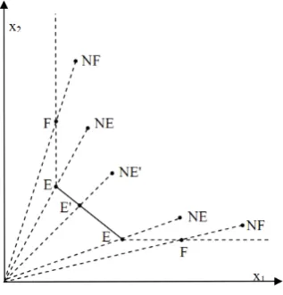
In DEA a set of DMUs are partitioned into two main classes: efficient and inefficient. The efficient units make the efficiency frontier. Figure 1 shows the classification of DMUs, based on the position of their reference on the efficiency frontier (Charnes et al., 1991).

Fig. 1: Classifying DMUs.

In this classification,EandEare efficient andNEandNEare inefficient DMUs. In addition, F and NF are weakly efficient and weakly inefficient, respectively.

Suppose that there are nDecision Making Units (DMUs) each consumes m inputs to produce s outputs. Let x_j = (x₁_j, x₂_j, . . . , x_mj) and y_j = (y₁_j, y₂_j, . . . , y_sj) are input vector and output vector of DMUj (j= 1, . . . , n), respectively. Hence, the CCR model corresponding to DMUp is as follow:

(3)

minz=θ−ε(Σ_im₌₁(s−_i ) +Σs_r₌₁(s+_r))

s.t.

xipθ−s−i −Σjn=1xijλj = 0,∀i

−s+

r +Σjn=1yrjλj =yrp,∀r

λj, s−i , s+r ≥0,∀i, r, j

To introduce the new method, all of the values of variables for all DMUs are needed. So consider the following integrated model.

CCRP Model:

minz=θ_p−ε(Σ_im₌₁s−_ip+Σ_rs₌₁s+_rp)

s.t.

xipθp−s−ip−Σjn=1xijλjp= 0, ∀i

−s+

rp+Σjn=1yrjλjp=yrp, ∀r

λjp, s−ip, s+rp≥0, ∀i, r, j

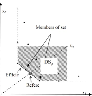
In the above model, for each variable an index has been added. To simplify the notation, letu_j= (y_j, x_j) be DMUj. Hence one can present members of productivity possibility set asu= (y,−x). Clearly,u_j ∈P P S,(j= 1, . . . , n). Let (θ∗_p, λ∗_p, s_p+∗, s−_p∗) is an optimal solution of CCR_p, then eﬃciency of u_p is equal toθ_p∗. We also denote the eﬃciency of ubyθ_u∗. The dominate space and reference of u_p are denoted by DS_p and u(p), respectively, and the set of reference indices ofu_pis denoted by E(p).

DSp={u∈P P S|u≥up}, u(p) =Σjn=1l∗jpuj, E(p) ={j:λ∗jp>0}

It is clear that u(p) ∈ DS_p and u(p) = Σ_j_∈_E₍_p₎λ∗_jpu_j. These concepts are illustrated in Figure 2.

The shading pattern in this ﬁgure and other ﬁgure in the paper represents the dominant space ofu_p, so every point in that region has inputs less than or equal and outputs more than or equal tou_p. And dashed line in the frontier is weakly frontier.

Therefore, we have:

(4)

Fig. 2: Eﬃcient frontier, dominate space, reference point and set of reference index.

3 New Method

As explained in previous section, for classifying the DMUs, the values ofθand slacks of reference point must be used. For eachu_p, two reference points are determined, the ﬁrst reference belongs toDS_pwhich minimizeθ_p. The second reference belongs toDS_p which maximizeΣ_im₌₁s_ip−∗+Σ_rs₌₁s+_rp∗. Consider the following models:

Model P1:

minz=θ_ps.t.

xipθp−Σnj=1xijλljp≥0, ∀i

Σn

j=1yrjλljp≥yrp, ∀r

λl

jp≥0, ∀j

Model P2:

minz=−(Σ_im₌₁s−_ip+Σ_rs₌₁s+_rp)

s.t.

s−_ip+Σ_jn₌₁x_ijλ2_jp=x_ip, ∀i −s+

rp+Σjn=1yijλ2jp=yrp, ∀i

λ2

(5)

The ﬁrst reference foru_pis determined by Model P1 asu₁(P) =Σ_jn₌₁λl_jp∗u_j. Similarly, the second reference for u_p is determined by the model p2 as

u2(p) =Σjn=1λ2

∗

jpuj. These references are illustrated in Figure 3:

Fig. 3:u_p and its ﬁrst and second references.

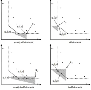
u1(p) is not always the same as the reference point which is defined as (θ∗x_j, y_j) for (x_j, y_j). Ifu_pbe an efficient or inefficient unit then its reference point andu₁(p) are the same and if it is a weakly efficient or inefficient unit then probably its reference probably its reference point and u₁(p) are not equal to each other. For example, in the Figure 4(a), u₁(p) and reference point ofu_pare the same, but if the weakly efficient unit u₁(p) is removed as illustrated in the Figure 4(b), the two definitions become different. In this case the reference point can be improved to the u₁(p), therefore we must improve the reference point, too. Reference of each unit must be on the (strong) frontier and not on the weakly frontier. Weakly frontier is shown by dashed line in the figures in the paper.

(6)

ˆ

u(p) =Σ_kn₌₁(Σ_jn₌₁λ1_jp∗λ2_kj∗)

Ifu_p be an efficient or an inefficient unit then the revised reference isu₁(p), but if it is a weekly efficient or inefficient unit then the reference for u_p on the frontier is moved by û(p) using the weights belonging to E(P). Revised reference is simply the second reference of the first reference of thepthunit. We introduce a simple algorithm to identify the revised reference of u_p and describe the idea of revised reference. It woks as follows:

1. Find the first reference ofu_p. There are one or more units that create the first reference ofu_p. They are efficient or weakly efficient units.

2. For each unit that participating the construction of the ﬁrst reference of

up, ﬁnd the second reference. For each of them, there are one or more units

that are eﬃcient (and not weakly eﬃcient).

3. The second reference of the first reference ofu_p is the actual reference of it, so calculate values of the new variable that create the second reference of the first reference ofu_p. The revised reference is on the efficient frontier and is the actual reference of u_p.

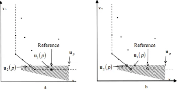
This algorithm computed the revised reference of u_p, in other word we move of u_p tou₁(p) and then move tou₂(u₁(p)), as illustrated in Figure 4.

Fig. 4: Reference point andu₁(p) may be diﬀerent.

These concepts lead to the next theorems 1 proves that only efficient (not weakly efficient) units participating in construction of revised reference. And theorem 2 proves that comparingu_pto the revised reference results the actual efficiency.

Theorem 3.1.If uk is not an eﬃcient unit then n_j₌₁λ1jp∗λ2

∗

(7)

Proof. Sinceλ2_kj∗ is the optimum weight ofu_k in the model P2 for evaluating

uj, if uk is a weakly efficient, an inefficient or a weakly inefficient unit then

for all j, λ2_kj∗ = 0 and n_j₌₁λ1_jp∗λ2_kj∗ = 0.

Theorem 3.2.If we select ˆu(p) as a reference forup in the model P1, then

eﬃciency value of up is equal to θp∗.

Proof. We knew thatu₁(p) is on the efficient frontier andθ_p∗is the minimum value ofθ_p, so we must prove that û(p)≥u₁(p). We rewrite the û(p) as follow:

ˆ

u(p) = n_j₌₁λ1_jp∗

⎧

⎩ n

j=1λ2

∗

kjuk ⎫

⎭ = n_j₌₁λ1_jp∗u₂(j), where u₂(j) is the reference ofu_j in the model P2.

There are three possibilities fors_j:

1. Ifu_j is an inefficient or a weakly inefficient unit, thenλ1_jp∗ = 0. 2. Ifu_j is an inefficient unit, thenλ1_jp∗ >0 andu₂(j) =u_j. 3. Ifu_j is an weakly unit, thenλ1_jp∗ >0 andu₂(j)≥u_j.

In all cases we have ˆu(p) =n_j₌₁λ1_jp∗u₂(j)≥n_j₌₁λ1_jp∗u_j =u(p).

Since θ∗_p is the minimum value of θ_p, therefore, if we select ˆu(p) as the reference ofu_pin model P1, the eﬃciency value of u_p is equal toθ∗_p.

This shows that û(p) is on the efficient frontier, andn_j₌₁λ1_jp∗λ2_kj∗ >0 if and only ifu_i is an efficient unit.

Based on Theorems 1 and 2, û(p) is a combination of (only) efficient units and its corresponding efficiency value is the same as in model P1. After applying models P1 and P2 for all units, it is possible to compute the revised references of all units, which are on the efficient (and not on the weakly efficient) frontier. It sounds that this method is similar two phase method, but in the new method, the two models are independent.

Based on theorems 1 and 2, û(p) is on the efficient frontier and as a ref-erence foru_p, the efficiency value is not changed. ˆλ∗_kp=_jn₌₁λ1_jp∗λ2_kj∗, where the related slacks are computed as follows:

ˆ

s−∗

ip =θp∗xip− n

j=1 ˆ

λ∗

jpxij, sˆ+rp∗= n

j=1 ˆ

λ∗

jpyrj−yrp.

Therefore, after applying P1 and P2 models for all units, we can compute the revised references, which are on the eﬃciency frontier, and the related slacks. According to classifying the DMUs, we have:

(8)

The reference for u_p is ˆu(p) =n_j₌₁λˆ∗_jku_j.

The basic role of this method is removing the non-Archimedean epsilon of models and using models that have no dependency to each others and could be solved separately while the models of two-phase method needs to be solved respectively, because second model uses of result of ﬁrst model.

The basis of traditional two-phase method is to find the optimum value of θ in the first stage and fix it to the second LP and solve it to find the maximum value for sum of slacks.

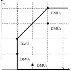
4 Numerical Example

In this section we solve a simple numerical example. We add the constraints

_n

j=1λ1jp= 1 and

_n

j=1λ2jp= 1 to models P1 and P2 respectively and create

the BCC versions of DEA models. Consider the following example:

Table 1:Data for the numerical example

Output y Inputx

DMU1 1 1

DMU2 2 1

DMU3 0.2 2

DMU4 3 3

DMU5 4 3

These data are illustrated in Figure 5.

(9)

Table 2 shows the optimum solutions of models P1 and P2 in the BCC format:

Table 2: Results of the example using model P1 and P2 with variable returns to scale

DMU θ∗ _λ1∗

λ2∗

1 2 3 4 5 1 2 3 4 5

DMU1 1 1 0 0 0 0 0 1 0 0 0

DMU2 1 0 1 0 0 0 0 1 0 0 0

DMU3 0.50 1 0 0 0 0 0 1 0 0 0

DMU40.6667 0 0.5 0 0 0.5 0 0 0 0 1

DMU5 1 0 0 0 0 1 0 0 0 0 1

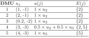
For example for DMU4, we haveλ2₂₄∗ = 0.5,λ₅₄2∗ = 0.5, and λ2₅₄∗ = 1. The following table presents ˆs−∗, ˆs+∗ and ˆλ∗:

Table 3: ˆs−∗, ˆs+∗ and ˆλ∗

DMUθ∗ _s_ˆ−∗

ˆ

s+∗ _ˆ

λ∗ 1 2 3 4 5 1 1 0.0 1.0 0 1 0 0 0 2 1 0.0 0.0 0 1 0 0 0 3 0.50 0.0 1.80 0 1 0 0 0 4 0.6667 0.0 0.0 0 0.5 0 0 0.5 5 1 0.0 0.0 0 0 0 0 1

Thus, the revised references of DMUs are as follow:

Table 4: The revised references of DMUs

DMUuj u(j) E(j) 1 (1, -1) 1×u2 {2} 2 (2, -1) 1_×_u₂ _{2_} 3 (0.2, -2) 1×u₂ {2} 4 (3, -3) 0.5×u2+ 0.5×u5 {2,5} 5 (4, -3) 1_×_u₅ _{5_}

(10)

5 Conclusion

There are two major methods for solving the basic DEA models: the epsilon based method, which selects a real number for epsilon, and the two phases method, which is used two LPs for each DMU. In this paper, we presented another method that determines two references for each DMU and then com-bines them and computes new lambdas and slack variables. Solving models without using non-Archimedean epsilon is an advantage of the new method and ability of computing the models in parallel can reduce the overall running time.

References

1. Ali, A.I. and Seiford, L. M.,Computational Accuracy and Inﬁnitesimals in Data En-velopment Analysis.INFOR,37, (1993), 290-297.

2. Alirezaee, M. R. and Khalili, M.,Recognizing the efficiency, weak efficiency and inef-ficiency of DMUs with an epsilon independent linear program.Applied Mathematics and Computation,183, (2006), 1323-1327.

3. Amin, G. R. and Toloo, M.,A polynomial-time algorithm for ﬁnding Epsilon in DEA models.Computers Operations Research,31, (2004), 803-805.

4. Banker, R. D., Charnes, A., and Cooper, W.W.,Some models for estimating techni-cal and stechni-cale ineﬃciencies in data envelopment analysis, Management Science,30, (1984), 1078-1092.

5. Charnes, A., Cooper, W. and Rhodes, E.,Measuring the Eﬃciency of Decision Making Units. European Journal of Operational Research,₂, (1978), 429-444.

6. Charnes, A., Cooper, W. and Thrall, R. M.,A Structure for Classifying and Char-acterizing Eﬃciency and Ineﬃciency in Data Envelopment Analysis.The Journal of Productivity Analysis,₂, (1991), 197-237.

7. Charnes, A. and Rhodes, E., Short Communication Measuring the Eﬃciency of DMU’s. EJOR (1979), 339-339.

8. Cooper, W. W., Seiford, L .M. and Tone, K., Data EnvelopmentAnalysis A Com-prehensive Text with Models., Applications, References and DEA-Solver Software, Springer Science, (1999).

9. Emrouznejad, A., Parer, B. R. and Tavarese, G.,Evaluation of research in eﬃciency and productivity: A survery and analysis of the ﬁrst 30 years of scholarly literature in DEA. Socio-Economic Planning Sciences,42, (2008), 151-157.

10. Mehrabian, S., Jahanshahloo, G. R., Alirezaee, M. R. and Amin, G. R.,An Assurance Interval for the Non-Archimedean Epsilon in DEA Models.Operations Research,48, (2000), 344-347.