The concept of B-efficient solution in fair multiob jective optimization problems

Galley

Pro

of

DOI: 10.22067/ijnao.v7i1.43960

The concept of

B-efficient solution in

fair multiobjective optimization

problems

D. Foroutannia∗ and A. Mahmodinejad

Abstract

A problem that sometimes occurs in multiobjective optimization is the existence of a large set of fairly efficient solutions. Hence, the decision making based on selecting a unique preferred solution is difficult. Considering models with fairB-efficiency relieves some of the burden from the decision maker by shrinking the solution set, since the set of fairlyB-efficient solutions is contained within the set of fairly efficient solutions for the same problem. In this paper, first some theoretical and practical aspects of fairlyB- efficient solutions are discussed. Then, some scalarization techniques are developed to generate fairlyB-efficient solutions.

Keywords: Fair optimization; Nondominated; Equitability; B-efficiency; Scalarization.

1 Introduction

The Multiobjective programming has been studied for many years and mul-tiobjective methods have found applications in diverse areas of human life. It is well-known that any multiobjective optimization problem starts usually with an assumption that the criteria are incomparable, i.e., different criteria may have different units and physical interpretations. Many applications, however, arise from situations which present equitable criteria. Equitability is based on the assumption that the criteria are not only comparable (mea-sured on a common scale) but also anonymous (impartial). The latter makes

∗_{Corresponding author}

Received 31 January 2015; revised 18 June 2016; accepted 23 July 2016 D. Foroutannia

Department of Mathematics, Vali-e-Asr University of Rafsanjan, Rafsanjan, Iran. e-mail: [email protected]

A. Mahmodinejad

Department of Mathematics, Sirjan University of Technology, Sirjan, Iran. e-mail: [email protected]

Galley

Pro

of

the distribution of outcomes among the criteria more important than the as-signment of outcomes to specific criteria, and therefore models fair allocation of resources.

The fair preference was first known as the generalized Lorenz domi-nance [5, 7]. Kostreva and Ogryczak [3] are the first ones who introduced the concept of equitability into multiobjective programming. They have shown fair efficiency to be a refinement of Pareto efficiency by adding, to the reflexivity, strict monotonicity and transitivity of the Pareto preference order, the requirements of impartiality and satisfaction of the principle of transfers. Then, Kostreva et al. [4] presented the theory of equitable effi-ciency in greater generality. They have developed scalarization approaches to generate equitably efficient solutions of linear and nonlinear multiobjec-tive programs. Ogryczak applied equitability to portfolio optimization [8], location problems [9, 12], and telecommunications [11]. Moreover Ogryczak et al. [10], applied fair (equitable) optimization methods for the resource allocation problems in communication networks.

It should be noted that some authors have used the term “equitable” rather than “fair”. In this paper, we investigate some theoretical and prac-tical aspects of the fairlyB-efficient solutions and propose some approaches to generate equitablyB-efficient solutions. The results are generalizations of the results of Kostreva and Ogryczak [3] and Kostreva et al. [4].

2 Terminology

Throughout this article, the following notation is used. Let Rm _{be the}

Eu-clidean vector space and y′, y′′ ∈ Rm. y′ ≦ y′′ denotes y_i′ ≤ y_i′′ for all

i= 1,· · · , m. y′ < y′′ denotesy′_i< y_i′′for all i= 1,· · ·, m. y′≤y′′ denotes

y′≦y′′ buty′̸=y′′.

Consider a decision problem defined as an optimization problem withm

objective functions. For simplification we assume, without loss of general-ity, that the objective functions are to be minimized. The problem can be formulated as follows:

{

min(f1(x), f2(x),· · ·, fm(x)),

subject to x∈X (1)

wherexdenotes a vector of decision variables selected from the feasible setX

andf(x) = (f1(x), f2(x),· · · , fm(x)) is a vector function that maps the

fea-sible setX into the objective (criterion) spaceRm_{. We refer to the elements}

Galley

Pro

of

In single objective minimization problems, we compare the objective val-ues at different feasible decisions to select the best decision. Decisions are ranked according to the objective values at those decisions and any deci-sion with smallest objective value is called an optimal solution. Similarly, to make the multiobjective optimization model operational, one needs to assume some solution concept specifying what it means to minimize multiobjective functions. The solution concepts are defined by the properties of the corre-sponding preference model. We assume that solution concepts depend only on the evaluation of the outcome vectors while not taking into account any other solution properties not represented within the outcome vectors. Thus, we can limit our considerations to the preference model in the objective space

Y.

In the following, some basic concepts and definitions of preference rela-tions are reviewed from [3]. Preferences are represented by a weak preference relation by⪯, which allows us to compare pairs of outcome vectorsy′,y′′in the objective space Y. We sayy′ ⪯y′′ if and only if “y′ is at least as good as y′′” or “y′ is weakly preferred toy′′”. In words, y′ ⪯y′′ means that the decision maker thinks that the outcome vector y′ is at least as good as the outcome vector y′′. It should be noticed that the weak preference relation, the “ at least as good as” relation, is given by the decision maker. From⪯, we can derive two other important relations onY.

Definition 1. Lety′, y′′ ∈ Rm _{and let ⪯be a relation of weak preference}

defined onRm_×Rm_{. The strict preference relation,≺, defined by}

y′≺y′′⇔(y′ ⪯y′′and not y′′⪯y′), (2) and read y′ is strictly preferred to y′′. Also the indifference relation, ≃, defined by

y′≃y′′⇔(y′⪯y′′and y′′⪯y′), (3) and ready′ is indifferent toy′′.

Hence “y′ is at least as good asy′′” means that “y′ is strictly preferred toy′′” or “y′ is indifferent toy′′”.

Definition 2. Preference relations satisfying the following axioms are called rational preference relations:

1. Reflexivity: for ally∈Rm_,y⪯y.

2. Transitivity: for ally′, y′′, y′′′ ∈Rm_,y′_⪯y′′_andy′′_⪯y′′′_⇒y′_⪯y′′′_.

3. Strict monotonicity: for ally ∈Rm,y−ϵei ≺y for allϵ >0 whereei

denotes theith_{unit vector inR}m_{, for alli∈ {1,2,· · ·, m}.}

Galley

Pro

of

iffy′≺y′′for all rational preference relations ⪯.

An outcome vectoryis rationally nondominated if and only if there does not exist another outcome vector y′ such that y′ rationally dominates y. Analogously, a feasible solution x ∈X is an efficient or Pareto-optimal so-lution of the multiobjective problem (1) if and only ify=f(x) is rationally nondominated.

It has been shown in [3] that the outcome vectory′ ∈Y rationally dom-inates y′′ ∈ Y if and only if y′ ≤ y′′. As a consequence, we can state that a feasible solution x∈X is a Pareto-optimal solution of the multiobjective problem (1), if and only if, there does not existx′ ∈Xsuch thatfi(x′)≤fi(x)

fori= 1,2,· · · , m, where at least one strict inequality holds. Let⪯be a preference relation defined onRm_.

Definition 4. ⪯is said to be impartial if

(y1, y2,· · · , ym)≃(yτ(1), yτ(2),· · ·, yτ(m))

for all y∈Rm_{, whereτ stands for an arbitrary permutation of components}

ofy.

Definition 5. ⪯ is said to satisfy the principle of transfers if yi > yj ⇒

y−ϵei+ϵej⪯y, for ally∈Rmand allϵ∈[0, yi−yj].

Definition 6. A preference relation⪯defined onRmis called a fair rational preference relation if it is reflexive, transitive, strictly monotonic, impartial and satisfies the principle of transfers.

The fair rational preference relations allow us to define the concept of fairly efficient solution.

Definition 7. Let y′, y′′ ∈ Y. We say that y′ fairly dominates y′′, and denote byy′≺ey′′ iffy′≺y′′for all fair rational preference relations⪯.

An outcome vectory is fairly nondominated if and only if there does not exist another outcome vectory′such thaty′fairly dominatesy. Analogously, a feasible solutionxis called a fairly efficient solution of the multiobjective problem (1) if and only ify=f(x) is fairly nondominated.

Definition 8. Lety∈Rm_.

1. The function Θ : Rm → Rm is called an ordering map iff Θ(y) = (θ1(y), θ2(y),· · ·, θm(y)), whereθ1(y)≥θ2(y)≥ · · · ≥θm(y) in whichθi(y) =

yτ(i)fori= 1,2,· · ·, m, andτ is a permutation of the set{1,2,· · ·, m}.

2. The function Θ : Rm → Rm is called a cumulative ordering map iff Θ(y) = (¯θ1(y),θ¯2(y),· · ·,θ¯m(y)), where ¯θi(y) =

∑i

j=1θj(y) for

Galley

Pro

of

To make it practical, fair efficiency is defined in terms of vector inequali-ties.

Proposition 1. ( [3], Proposition 2.3) For any two vectors y′, y′′∈Y y′⪯ey′′⇔Θ(y′)≦Θ(y′′),

where⪯e is given by Definition 7.

3 Fair

B-efficient solutions

In this section, we first introduce the concept of fairly B-efficient solution by fair rational preference relations. Then, similar to the fair dominance relation, we can express the fair B-dominance relation in terms of vector inequality on the ordered outcome vectors.

In fair multiobjective optimization, the focus is on the distribution of outcome values while ignoring their ordering. This means that in the mul-tiobjective optimization problem (1) we are interested in a set of values of the objectives without taking into account which objective is taking a specific value. In this respect, let {1,2,· · ·, m} be the index of the vector Θ(y) = (θ1(y), θ2(y),· · ·, θm(y)) andnbe a positive integer such thatn≤m.

Throughout this article, we suppose thatB ={B1, B2,· · · , Bn}is a partition

of the set{1,2,· · ·, m} such that

maxBi<minBi+1, i= 1,2,· · ·, n−1. (4)

The following definition is a necessary notion for the solution concepts of interest in this paper.

Definition 9. Suppose that n ≤ m and B = {B1, B2,· · · , Bn} is a

par-tition of {1,2,· · ·, m} such that condition (4) is satisfied. The cumulative map ΘB:Rm→Rn is defined by

ΘB(y) =



∑

j∈B1

θj(y),

∑

j∈B2

θj(y),· · · ,

∑

j∈Bn

θj(y)

 ,

whereθj’s are as defined in Definition 8.

Definition 10. Suppose that y′, y′′ ∈ Y are two outcome vectors. We say that y′ fairlyB-dominates y′′ and write y′≺Bey′′ iff ΘB(y′)≺ΘB(y′′)

for all fair rational preference relations⪯.

Galley

Pro

of

iff there does not existy′∈Y such thaty′≺Bey.

Definition 12. We say that feasible solution x ∈ X is a fairly B -efficient solution of the multiobjective problem (1), iff y = f(x) is fairly

B-nondominated.

Similar to the relation of fairB-dominance, we can define the relation of fairB-indifference (indifference for all fair rational preference relations) and the relation of fair weak B-dominance (weak preference for all fair rational preference relations). The relations of fairB-dominance≺Be,B-indifference

≃Be, and weakB-dominance⪯Be satisfy conditions (2-3).

To make it practical, fairB-efficiency can be defined in terms of vector inequalities. In order to do that, we define certain mapping.

Definition 13. Suppose that n ≤m and B = {B1, B2,· · ·, Bn} is a

par-tition of {1,2,· · ·, m} such that condition (4) is satisfied. The cumulative ordering map ΘB:Rm→Rn is defined by

ΘB(y) =



∑

j_∈B1

θj(y),

∑

j_∈B_1∪B2

θj(y),· · ·,

∑

j_∈B_1∪B_{2∪···∪}Bn

θj(y)

 ,

whereθj’s are as defined in Definition 8.

Definition 14. Suppose that y′, y′′ ∈ Y are two outcome vectors. The relation≤Bie is defined as follows.

y′≤Biey′′⇔ΘB(y′)≦ΘB(y′′).

Note that if Bj = {j} for j = 1,2,· · · , m, then ΘB(y) = Θ(y) and

ΘB(y) = Θ(y), so the relation⪯Be becomes the relation⪯e.

The relations<Bie and =Bie are defined by

y′ <Bie y′′⇔(y′ ≤Biey′′and not y′′≤Biey′),

y′ =Bie y′′⇔(y′ ≤Biey′′and y′′≤Biey′).

Below, we will discuss the relationship between two preference relations ⪯Be and≤Bie. In order to do that, we need the following proposition.

Proposition 2. ( [3], Proposition 2.2) If Θ(y′) ≤ Θ(y′′), then Θ(y′) ≤ Θ(y′′) or there exists a finite sequence of vectors y0 _{= y}′′_{, y}1_{,· · ·, y}t _such

that yk _=yk−1_−ϵ

kei′ +ϵkei′′, i′, i′′ ∈ {1,2,· · ·, m},0< ϵk < y_ik′−1−y_ik′′−1

fork= 1,2,· · · , tandΘ(y′)≦Θ(yt_).

Galley

Pro

of

Θ(y′)≦Θ(y′′) =⇒Θ(y′)⪯Θ(y′′).

Theorem 1. Let |B1| ≥ |B2| ≥ · · · ≥ |Bn| and y′, y′′ ∈ Y be two outcome

vectors. We have

y′ ⪯Bey′′⇐⇒y′ ≤Bie y′′,

y′ ≺Bey′′⇐⇒y′ <Bie y′′.

Proof. By assumption|B1| ≥ |B2| ≥ · · · ≥ |Bn|, we have

∑

j_∈B1

θj(y)≥

∑

j_∈B2

θj(y)≥ · · · ≥

∑

j_∈Bn

θj(y),

for ally∈Y. This means that the vector ΘB(y) is decreasing, so Θ(ΘB(y)) =

ΘB(y). It is clear that

y′⪯Bey′′=⇒y′≤Biey′′,

since the relation⪯eis a fair rational preference relation. Conversely suppose

that y′ ≤Bie y′′, we deduce ΘB(y′)≦ΘB(y′′). So

Θ(ΘB(y′))≦Θ(ΘB(y′′)).

Due to Proposition 2, we have ΘB(y′)⪯ΘB(y′′) for any fair rational

pref-erence relation⪯. Thusy′⪯Bey′′. By the same reasoning, remaining cases

are satisfied.

Due to Theorem 1, we deduce that the relation ⪯Be is a fair rational

preference relation, when|B1| ≥ |B2| ≥ · · · ≥ |Bn|. Preference relation⪯Be,

in general, does not satisfy the principle of transfers axiom. The truth of this statement is examined by the following example.

Example 1. Let B1 = {1}, B2 = {2,3}, y = (4,2.5,2). If ϵ = 1 and

y′ = y−ϵe1+ϵe3, then y′ = (3,2.5,3). Since Θ(ΘB(y)) = (4.5,8.5) and

Θ(ΘB(y′)) = (5.5,8.5). We have Θ(ΘB(y′))≦̸Θ(ΘB(y)), soy′⪯̸Bey.

It should be noted that in this example ΘB(y) = (4,8.5) and ΘB(y′) =

(3,8.5). Soy′≤Bie y. Also ify′ = (4,2,1) andy′′= (3.5,3,2), it is obvious

thaty′ ⪯Bey′′while they′≰Biey′′. This reflects the fact that Theorem 1, in

general, is not true for any partitionBand condition|B1| ≥ |B2| ≥ · · · ≥ |Bn|

is necessary.

By applying Theorem 1 and Definition 14, we have the following statement.

Corollary 1. Suppose that |B1| ≥ |B2| ≥ · · · ≥ |Bn| and y′, y′′ ∈ Y.

Galley

Pro

of

y′⪯Bey′′⇔ΘB(y′)≦ΘB(y′′),

y′≺Bey′′⇔ΘB(y′)≤ΘB(y′′).

Remark 1. IfBj={j}forj= 1,2,· · · , m, we have Proposition 2.3 from [3].

Note that Corollary 1 permits one to express fairB-efficiency for problem (1) in terms of the standard efficiency for the multiobjective problem with objectives ΘB(f(x)):

min{ΘB(f(x)) :x∈X}. (5)

Theorem 2. Let |B1| ≥ |B2| ≥ · · · ≥ |Bn|. A feasible solutionx∈X is a

fairly B-efficient solution of the multiobjective problem (1) if and only if it is an efficient solution of the multiobjective problem (5).

Proof. By applying Corollary 1, we obtain the desired result.

Remark 2. If Bj = {j} for j = 1,2,· · ·, m, then we have Corollary 2.2

from [3].

The following theorem provides the relationship between fairlyB-efficient solutions and fairly efficient solutions.

Theorem 3. Let |B1| ≥ |B2| ≥ · · · ≥ |Bn|and y ∈Y be a outcome vector.

If y is fairly B-nondominated, then it is fairly nondominated.

Proof. Suppose thatyis not fairly nondominated. Then there exists a vector

y′ ∈Y such thaty′≺ey. Due to Proposition 1, Θ(y′)≤Θ(y), soy′<Bie y.

Since|B1| ≥ |B2| ≥ · · · ≥ |Bn|, by using Corollary 1, we deduce that y′≺Be

y.

Corollary 2. Let|B1| ≥ |B2| ≥ · · · ≥ |Bn|andx∈X be a feasible solution.

Ifxis a fairlyB-efficient solution of multiobjective problem (1), then it is an fairly efficient solution of (1).

This result suggests that the set of fairlyB-efficient solutions is contained within the set of fairly efficient solutions, but the reverse inclusion doesn’t hold in general. It should be noted the structure of fair dominance is dis-cussed in Example 2.1 of [3] by Kostreva and Ogryczak. They showed that the set of fairly efficient solutions is contained within the set of efficient so-lutions. In the following examples, we investigate the effectiveness of fair

B-dominance relation with respect to fair dominance.

Example 2. Let’s consider the problem

min{(x1, x2) : 4x1+ 5x2≥72, x1≥0,0≤x2≤72/5},

Galley

Pro

of

E={(x1, x2) : 4x1+ 5x2= 72, x1≥0, x2≥0},

F={(x1, x2) : 4x1+ 5x2= 72,0≤x1≤8,8≤x2≤72/5},

andG={(0,72/5)}are the set of efficient solutions, the set of fairly efficient solutions and the set of fairly B-efficient solutions, respectively. Thus G⊊ F ⊊E.

In the next example, a large number of random solutions are generated for scalable test functions. From this large set of solutions, the nondomi-nated solutions with respect to rational dominance (Pareto dominance), fair dominance and fairB-dominance are calculated.

Example 3. The test problem considered is the VFM1 [14], min

x_∈R2y={f1(x), f2(x), f3(x)}

f1(x) =x21+ (x2−1)2

f2(x) =x21+ (x2+ 1)2+ 1

f3(x) =(x1−1)2+x22+ 2

x1, x2∈[−2,2].

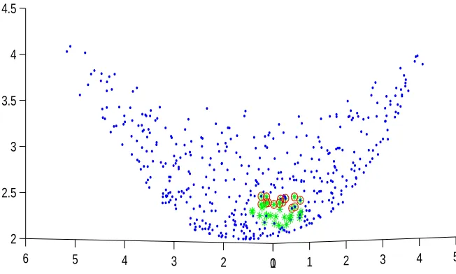
Figure 1 shows the Pareto, fair and fair B-dominance fronts (objective space).

0 1 2 3 4 5

1 2

3 4

5 6

2 2.5 3 3.5 4 4.5

Galley

Pro

of

From 5000 random solutions, 496 solutions (point) are rationally non-dominated, 37 solutions (star) are fairly nondominated and 14 solutions (circle) are fairly B-nondominated, which are obtained by assuming B1 =

{1,2}, B2={3}.

In the rest of this section, we will investigate the structure of fairly B -efficient set. For this purpose, problem (1) is considered as a multiobjective linear programming problem. It is assumed that,X ⊂Rndenotes the feasible set defined by a system of linear equations and inequalities, and the objective functions are

fi(x) =cix (i= 1,2,· · ·, m), (6)

wherecT

i ∈Rn. Suppose thatn≤mandB ={B1, B2,· · · , Bn}is a partition

of{1,2,· · ·, m} such that condition (4) is satisfied. We putbi= maxBi for

i= 1,2,· · · , n, so ΘB(y) =

 ∑b1

j=1

θj(y), b2

∑

j=1

θj(y),· · · , bn

∑

j=1

θj(y)

 

=(θ¯b1(y),θ¯b2(y),· · ·,θ¯bn(y)

)

,

where ¯θbi(y) =

∑bi

j=1θj(y) for i= 1,2,· · ·, n, andbn =m. In Theorem 2,

we established the equivalence between the fairly B-efficient solutions of (1) and the efficient solutions of problem (5). Now, we further use this result to explore the structure of the fairly B-efficient set. Note that the individual objective functions of problem (5) are convex piecewise linear functions of

y=f(x). They can be written in the form ¯

θbi(y) = max_τ

∈Π  ∑bi

j=1

yτ(j) 

 (i= 1,2,· · ·, n), (7) where Π denotes the set of all permutationsτof the set{1,2,· · · , m}. Thus, the corresponding problem (5) can be expressed in the form of multiobjective linear program

min (zb1, zb2,· · · , zbn) (8)

subject to

x∈X, (9)

yi=cix f or i= 1,2,· · · , m, (10)

zbi ≥

bi

∑

j=1

Galley

Pro

of

Put zB= (zb1, zb2,· · · , zbn). According to (7), the problem above is

equiva-lent to problem (5) as stated in the following theorem.

Theorem 4. A triple (x, y, zB) is an efficient solution of (8)-(11), if and

only ify=Cx ,zB = ΘB(y)andxis an efficient solution of the

multiobjec-tive problem (5).

Remark 3. If Bj = {j} for j = 1,2,· · ·, m, then we have Proposition

4.1 from [3].

The question that arises is whether there exist fairlyB-efficient solutions. The next result provides some sufficient conditions to answer this question. For this purpose, we need the following theorem.

Theorem 5. ( [1], Theorem 6.5) IfX ̸=∅and there existsy0∈Y such that

y0≤Cxfor all x∈X, then there exists a efficient solution of problem (1).

Theorem 6. Let |B1| ≥ |B2| ≥ · · · ≥ |Bn|. If X ̸= ∅ and there exists

y0 _{∈ Y such that y}0 _⪯

Be Cx for all x ∈ X, then there exists a fairly B

-efficient solution of problem (1).

Proof. Due to Corollary 1, z0

B = ΘB(y0) ≦ ΘB(Cx) for allx ∈ X. Thus,

z0

B ≦zBfor any attainable achievement vectorzBof the multiobjective linear

programming (8)-(11), which is by Theorem 4 equivalent to the problem (5). Hence, by using Theorem 5, there exists an efficient solution x0 _{of (8)-(11).}

Due to Corollary 1,x0 _{is a fairlyB-efficient solution of problem (1).}

Remark 4. If Bj ={j} forj = 1,2,· · ·, m, then we have Proposition 4.3

from [3].

Kostreva and Ogryczak in [3] have shown that the set of fairly efficient solutions is nonempty provided that the set of efficient solutions is nonempty.

Proposition 3. ( [3], Proposition 4.4) If there exists an efficient solution of problem (1), then there exists a fairly efficient solution of problem (1).

By applying Corollary 2 and Proposition 3, we obtain the following state-ment.

Corollary 3. Let |B1| ≥ |B2| ≥ · · · ≥ |Bn|. If there exists an efficient

solution of problem (1), then there exists a fairlyB-efficient solution of prob-lem (1).

In addition to the existence of the fairlyB-efficient set and its relationship to the efficient set, we investigate the fact that the fairly B-efficient set is connected. To do so, we need the following theorem.

Galley

Pro

of

multiobjective linear programming problem (8)-(11) is nonempty. Then the set of fairly B-efficient solutions of problem (1) is connected.

Proof. The set of fairlyB-efficient solutions of problem (1) is the same as the set of efficient solutions of problem (5). By using Theorem 4, the efficient solutions of problem (5) are in one-to-one correspondence to the efficient solutions of (8)-(11) . Since (8)-(11) is a linear multiobjective optimization problem, its efficient set is a connected set according to Theorem 7.

Remark 5. If Bj ={j} forj = 1,2,· · ·, m, then we have Proposition 4.5

from [3].

4 Generation techniques

In this section, we develop some scalarization-based methods to generate fairly B-efficient solutions. Scalarization is one of the most common ap-proaches used to solve a multiobjective problem. Scalarizing functions are used to transform a given multiobjective problem into a single objective opti-mization problem, by aggregating the objectives of a multiobjective problem into a single objective. Typical solution concepts for multiobjective problems are defined by scalarizing functions s : Y →R to be minimized. Thus the multiobjective problem (1) is replaced with the minimization problem

min{s(f(x)) : x∈X}. (12) The preference relation corresponding to the problem (12) is defined as follows:

y′⪯y′′⇔s(y′)≤s(y′′).

For any strictly convex, increasing functiong:R→R, the scalarizing func-tion defined by

s(y) =

m

∑

i=1

g(yi)

is a strictly monotonic and strictly Schur-convex function [7]. It has been shown in Proposition 3.1 from [3] that the preference relation corresponding to this scalarizing function is a fair rational preference relation. Also, every optimal solution of problem (12) is a fairly efficient solution of the original multiobjective problem.

In the following, we will generate the fairlyB-efficient solutions by intro-ducing certain scalarizing functions.

Galley

Pro

of

j∈Bi

θj(f(x))



: x∈X

 

, (13)

is a fairly B-efficient solution of the multiobjective problem (1).

Proof. Suppose thatxis not a fairlyB-efficient solution of the multiobjective problem (1). Then a feasible vectorx′ must exist such that the vectors f(x) and f(x′) satisfy f(x′) ≺Be f(x). Namely for all fair rational preference

relations ≺, we have ΘB(f(x′))≺ΘB(f(x)). Since the preference relation

corresponding to scalarizing function is a fair rational preference relation, we deduce that n ∑ i=1 g  ∑

j∈Bi

θj(f(x′))

 < n ∑ i=1 g  ∑

j∈Bi

θj(f(x))

 ,

which contradicts the optimal solution ofxfor (13).

Remark 6. IfBj={j} forj= 1,2,· · ·, m, we have Corollary 3.1 from [3].

The weighted sum method is one of the most common ways of finding efficient solutions of multiobjective problem. Details of the method can be found in [2]. Further, Kostreva et al. [4] have proven every optimal solution of the weighted sum problem with strictly decreasing positive weights and ordering map Θ(f(x)), is a fairly efficient solution of the original multiobjec-tive optimization problem. If the weighted sum method is applied to problem (5), due to the definition of map ΘB, we have

min    n ∑ i=1 wi   ∑

j∈B1∪B2∪···∪Bi

θj(f(x))



:x∈X

 

 (14)

wherew∈Rn is any positive vector. The above problem is equivalent to min    n ∑ i=1 λi  ∑

j_∈Bi

θj(f(x))



:x∈X

 

 (15)

whereλi=

∑n

j=iwj fori= 1,· · ·, n.

Theorem 10. Let λ1 > λ2 > · · · > λn > 0. If |B1| ≥ |B2| ≥ · · · ≥ |Bn|,

then the optimal solution of problem (15) is a fairly B-efficient solution of the multiobjective problem (1).

Galley

Pro

of

∑

B1∪···∪Bk

θj(f(x′))⩽

∑

B1∪···∪Bk

θj(f(x)) k= 1,2,· · ·, n,

where strict inequality holds at least once. Ifwi=λi−λi+1, thenwi>0 for

i= 1,2,· · · , n. So,

n

∑

k=1

wk

∑

B1∪···∪Bk

θj(f(x′))< n

∑

k=1

wk

∑

B1∪···∪Bk

θj(f(x)).

This means that x cannot be the optimal solution of problem (14). Since problems (14) and (15) are equivalent, the desired result is obtained.

Remark 7. If Bj = {j} for j = 1,2,· · ·, m, then we have Theorem 2

from [4].

A very important result in multobjective linear optimization is the as-sociation of efficient solutions with optimal solutions of the scalar weighting problem using positive weights [13]. The following result is the analogue for our fairly B-efficient solution set. It seems that such a result should thus play an important role in analysis of fairB-efficiency.

Theorem 11. Suppose that |B1| ≥ |B2| ≥ · · · ≥ |Bn| and the function

f is defined as in (6). A feasible solution x0 _{is a fairly B-efficient}

solu-tion of problem (1), if and only if, there exists a weight vector λ∈Rn _with

λ1> λ2>· · ·> λn>0such thatx0 is an optimal solution of problem (15).

Proof. Sufficiency of the condition follows from Theorm 10. Thus we only need to show that for each fairlyB-efficient solutionx0_{there exists a weight}

vector λ ∈ Rn _{with λ}

1 > λ2 > · · · > λn > 0 such that x0 is an optimal

solution of the problem (15). Due to Theorms 2 and 4, if x0 _{is a fairly B}

-efficient solution of (1), then (x0, Cx0,ΘB(Cx0)) is an efficient solution of

multiobjective linear program (8)-(11). Thus, from the theory of multiobjec-tive linear optimization [13], there exist posimultiobjec-tive weightsw1, w2,· · ·, wn such

that (x0, Cx0,ΘB(Cx0)) is an optimal solution of the problem

min

{ _n

∑

i=1

wizbi: (8)−(11)

}

(16)

Due to positive weightswi, the above problem is equivalent to the problem

min

{ _n

∑

i=1

wiθbi(Cx) : (8)−(11)

}

(17)

where ¯θbi(y) =

∑bi

j=1θj(y) fori= 1,2,· · · , n. Problem (17) is equivalent to

problem (15) whereλi=

∑n

j=iwj fori= 1,· · ·, n. This completes the proof

Galley

Pro

of

from [3].

Another way to generate fairlyB-efficient solutions is lexicographic min-imax approach. It is shown that any optimal solution of the lexicographic minimax problem is fairly efficient for the original multiobjective problem [4]. When applying the lexicographic optimization to the problem (5), we get the lexicographic problem

lexmin{ΘB(f(x)) :x∈X}. (18)

Due to Definition 13, problem (18) is equivalent to the problem

lexmin{ΘB(f(x)) :x∈X}. (19)

We recall that, if y′ ̸=y′′ and s= min{i :y_i′ ̸=y′′_i}, then y′ <lex y′′ if and

only ify′_s< y′′_s. Alsoy′≤lexy′′ if and only ifys′ < ys′′ory′ =y′′.

Definition 15. A feasible solution x ∈ X is lexicographically optimal or a lexicographic solution of the multiobjective problem (18), if there is no

x′∈X such that ΘB(f(x′))<lex ΘB(f(x)).

Theorem 12. Let x ∈ X be a lexicographically optimal solution of the multiobjective problem (18). Then x is a fairly B-efficient solution of the multiobjective problem (1).

Proof. Suppose thatxis not a fairlyB-efficient solution of the multiobjective problem (1). Then there exists a feasible vectorx′such thatf(x′)≺Bef(x).

Due to Corollary 1, ΘB(f(x′))≤ΘB(f(x)). So

∑

j∈B1∪B2∪···∪Bk

θj(f(x′))<

∑

j∈B1∪B2∪···∪Bk

θj(f(x)),

for somek∈ {1, ..., r}. Defining

s= min

  k:

∑

j∈B1∪B2∪···∪Bk

θj(f(x′))<

∑

j∈B1∪B2∪···∪Bk

θj(f(x))

  .

we get _∑

j_∈B_1∪B_{2∪···∪}Bk

θj(f(x′)) =

∑

j_∈B_1∪B_{2∪···∪}Bk

θj(f(x)),

fork= 1,2,· · · , s−1 and

∑

j∈B1∪B2∪···∪Bs

θj(f(x′))<

∑

j∈B1∪B2∪···∪Bs

Galley

Pro

of

Therefore ΘB(f(x′))<lexΘB(f(x)) contradicting the lexicographic

optimal-ity of x.

Remark 9. If Bj = {j} for j = 1,2,· · ·, m, then we have Corollary 3.3

from [3].

Since an efficient solution with equal outcomes is a lexicographic minimax solution. By Theorm 12, such a solution is fairlyB-efficient.

Corollary 4. If there exists any efficient solution x0 _{of problem (1) with}

equal outcomesf1(x0) =f2(x0) =· · ·=fm(x0), then it is a fairlyB-efficient

solution.

5 Conclusion

In this paper, we introduced a theoretical development of a new concept of solution of a multiobjective optimization problem. The concept of fair

B-efficiency is obtained from fair rational preference relations on a certain cumulative ordered vector. We introduced a new multiobjective optimization problem and by seeking efficient solutions of this new problem, we found fairly

B-efficient solutions of the original problem. Furthermore, we examined some properties of the set of fairly B-efficient solutions. These include sufficient conditions for existence, connectivity of the fairlyB-efficient set, scalarization methods, and characterizations related to weighting problems.

References

1. Ehrgott, M.Multicriteria optimization, Springer Verlag, Berlin, 2005. 2. Geoffrion, A. M.Proper efficiency and the theory of vector maximization,

Journal of Mathematical Analysis and Applications 22 (1968), 618-630. 3. Kostreva, M.M., and Ogryczak, W.Linear optimization with multiple

eq-uitable criteria, RAIRO Operations Research 33 (3) (1999), 275-297.

4. Kostreva, M.M., Ogryczak, W., and Wierzbicki, A.Equitable aggregations in multiple criteria analysis, European Journal of Operational Research 158 (2) (2004), 362-377.

5. Lorenz, M.O.Methods of measuring the concentration of wealth, American Statistical Association, New Series 70 (1905), 209-219.

Galley

Pro

of

7. Marshall, A.W., and Olkin, I. Inequalities: Theory of Majorization and Its Applications, Academic Press, New York, 1979.

8. Ogryczak, W. Multiple criteria linear programming model for portfolio selection, Annals of Operations Research 97 (2000), 143-162.

9. Ogryczak, W. Inequality measures and equitable approaches to location problems, European Journal of Operational Research 122 (2) (2000), 374-391.

10. Ogryczak, W., Luss, H., Pioro, M., Nace, D., and Tomaszewski, A.Fair optimization and networks: a survey, Journal of Applied Mathematics 2014 (2014), Article ID 612018, 25 pages.

11. Ogryczak, W., Wierzbicki, A., and Milewski, M. A multi-criteria ap-proach to fair and efficient bandwidth allocation, Omega 36 (2008), 451-463.

12. Ogryczak, W., and Zawadzki, M. Conditional median: a parametric so-lution concept for location problems, Annals of Operations Research 110 (2002), 167-181.

13. Steuer, R.E. Multiple Criteria Optimization Theory, Computation and Applications, John Wiley and Sons, New York, 1986.

۲_{داﮋﻧ یدﻮﻤﺤﻣ ﯽﻠﻋ و}۱_{ﺎﯿﻧ ﻦﺗوﺮﻓ دواد}

ﯽﺿﺎﯾر هوﺮﮔ ،نﺎﺠﻨﺴﻓر ﺮﺼﻌﯿﻟو هﺎﮕﺸﻧاد۱

ﯽﺿﺎﯾر هوﺮﮔ ،نﺎﺟﺮﯿﺳ ﯽﺘﻌﻨﺻ هﺎﮕﺸﻧاد۲

١٣٩۵ دادﺮﻣ ٢ ﻪﻟﺎﻘﻣ شﺮﯾﺬﭘ ،١٣٩۵ دادﺮﺧ ٢٩ هﺪﺷ حﻼﺻا ﻪﻟﺎﻘﻣ ﺖﻓﺎﯾرد ،١٣٩٣ ﻦﻤﻬﺑ ١١ ﻪﻟﺎﻘﻣ ﺖﻓﺎﯾرد

یﺎﻫباﻮﺟ زا گرﺰﺑ یاﻪﻋﻮﻤﺠﻣ دﻮﺟو ﺪﻫدﯽﻣ خر ﻪﻓﺪﻫﺪﻨﭼ یزﺎﺳﻪﻨﯿﻬﺑ رد ﻊﻗاﻮﻣ ﯽﻫﺎﮔ ﻪﮐ یاﻪﻠﺌﺴﻣ: هﺪﯿﮑﭼ

.ﺖﺳا ﻞﮑﺸﻣ دﺮﻔﺑﺮﺼﺤﻨﻣ هﺪﺷ هداد ﺢﯿﺟﺮﺗ باﻮﺟ بﺎﺨﺘﻧا ﺮﺑ ﯽﻨﺒﻣ یﺮﯿﮔ ﻢﯿﻤﺼﺗ وﺮﻨﯾا زا .ﺖﺳا ﻒﺼﻨﻣ ﺮﺛﻮﻣ ﻪﻋﻮﻤﺠﻣ ندﺮﮐ ﮏﭼﻮﮐ ﻪﻠﯿﺳو ﻪﺑ ار یﺮﯿﮔﻢﯿﻤﺼﺗ رﺎﺑ زا ﯽﻤﮐ ،ﻒﺼﻨﻣ یﺮﺛﻮﻣ-Bﺎﺑ هﺪﺷ ﻪﺘﻓﺮﮔﺮﻈﻧرد یﺎﻫلﺪﻣ یﺎﻫباﻮﺟ زا یاﻪﻋﻮﻤﺠﻣﺮﯾز ﻒﺼﻨﻣ ﺮﺛﻮﻣ-Bیﺎﻫباﻮﺟ ﻪﻋﻮﻤﺠﻣ ﻪﻠﺌﺴﻣ ﺮﻫ یاﺮﺑ نﻮﭼ ،ﺪﻨﮐﯽﻣ ﻢﮐ باﻮﺟ ﺚﺤﺑ ﻒﺼﻨﻣ ﺮﺛﻮﻣ-B یﺎﻫباﻮﺟ ﯽﻠﻤﻋ و یرﻮﺌﺗ ﻢﯿﻫﺎﻔﻣ زا ﯽﻀﻌﺑ اﺪﺘﺑا ،ﻪﻟﺎﻘﻣ ﻦﯾا رد .ﺖﺳا ﻒﺼﻨﻣ ﺮﺛﻮﻣ هداد ﻪﻌﺳﻮﺗ ﻒﺼﻨﻣ ﺮﺛﻮﻣ-B یﺎﻫباﻮﺟ ﺪﯿﻟﻮﺗ یاﺮﺑ یزﺎﺳیدﺪﻋ یﺎﻫﮏﯿﻨﮑﺗ زا ﯽﻀﻌﺑ ،ﺲﭙﺳ .ﺖﺳا هﺪﺷ ﺖﺳا هﺪﺷ