DOI:10.5545/sv-jme.2019.6350 Original Scientific Paper Accepted for publication: 2019-10-22
Review Paper —DOI: 10.5545/sv-jme.2017.4027 Accepted for publication: 2017-02-12
Multi-Physics and Multi-Scale Meshless Simulation System for
Direct-Chill Casting of Aluminium Alloys
Božidar Šarler1,2*- Tadej Dobravec2- Gašper Glavan1- Vanja Hati´c1,2- Boštjan Mavriˇc1,2- Robert Vertnik2 -Peter Cvahte3- Filip Gregor3- Marina Jelen3- Marko Petroviˇc3
1University of Ljubljana, Faculty of Mechanical Engineering, Slovenia
2Institute of Metals and Technology, Slovenia
3IMPOL 2000, d.d., Slovenia
This paper represents an overview of the elements of the user-friendly simulation system, developed for computational analysis and optimization of the quality and productivity of the electromagnetically direct-chill cast semi-products from aluminium alloys. The system also allows the computational estimation of the design changes of the casting equipment. To achieve this goal, the electromagnetic and the thermofluid process parameters are coupled to the evolution of Lorentz force, temperature, velocity, concentration, strain and stress fields as well as microstructure evolution. This forms a multi-physics and multi-scale problem of great complexity, which has not been demonstrated before. The macroscopic fluid mechanics, solid mechanics, and electromagnetic solution framework is based on local strong-form meshless formulation, involving the radial basis functions and monomials as trial functions, and local collocation or weighted least squares approximation. It is coupled to the micro-scale by incorporating the point automata solution concept. The entire macro-micro solution concept does not require meshing and space integration. The solution procedure can be easily and efficiently automatically adapted in node redistribution and/or refinement sense, which is of utmost importance when coping with fields exhibiting sharp gradients, which occur in the phase-change problems. The simulation system is coded from scratch in modern Fortran. The elements of the experimental validation of the system and the demonstration of its use for round billet casting in IMPOL Aluminium Industry are shown.
Keywords: direct-chill casting, aluminium alloys, computational solid and fluid mechanics, multi-physics modelling, multi-scale modelling, meshless methods, point automata method
Highlights
• Multiphysics and multi-scale simulation system for DCC with topmost capabilities. • Solution procedure based on originally developed meshless methods.
• Possibility of virtual computational changes in caster design and product properties.
0 INTRODUCTION
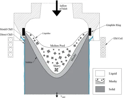
Direct-chill casting (DCC) (see Fig. 1) represents the most important process for production of aluminium alloys [1]. The process involves molten metal being fed vertically through a bottomless, water-cooled mould where it is sufficiently solidified around the outer surface to take the shape of the mould and acquire sufficient mechanical strength to contain the molten
core at the centre. As the strand emerges from
the mould, water impinges directly from the mould onto the surface, flows over the cast surface and
completes the solidification [2]. The technology,
despite being almost hundred years old, is still prone to different defects of the products such as porosity, macrosegregation, hot tearing, surface non-homogeneity, shape defects, and cracking. The additional action of the external fields such as electromagnetic, ultrasound, and mechanical stirring is used in the contemporary DCC devices. The casthouse
Fig. 1.Scheme of the DCC process
1 SIMULATION SYSTEM OVERVIEW
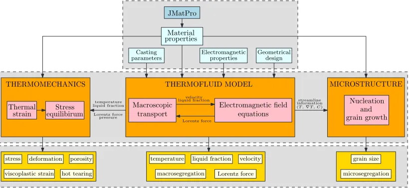
The overview of the simulation system is shown in Fig. 2. From the user perspective, three steps are required. The graphical user interfaces are provided for each step. The first step is the configuration of the input parameters and the material properties
[3], the second step is the simulation run and the
final step is inspection of the results. Internally,
the simulation system consists of four coupled modules. The calculation starts with fully coupled electromagnetic and thermofluid models, described in Section 2. Obtained results are then used as inputs for thermomechanical model, described in Section 3 and microstructure model, described in Section 4.
The nature of the coupling between the simulation
system modules is illustrated in Fig. 3. The
thermofluid model considers a limited part of the casting device, focused around the casting head, where the solidification takes place. The temperature field, solid fraction and pressure field are forwarded to Eulerian thermomechanical model, where the computational domain is restricted to the coherent part of the solid material, delimited by dashed lines in Fig. 3.
The microstructure model requires the thermal and chemical history of a piece of material to be extracted from the thermofluid model along a material
pathline. Several possible pathline selections are
indicated in Fig. 3 with white lines.
The outputs of each module are listed in Fig. 2. They are provided to the casting engineer in a report-like format. In this paper, the results are shown in the form of representation-friendly plots.
2 THERMOFLUID MODEL
The macroscopic equations for the conservation of mass, momentum, heat, and species are solved in the thermofluid model. The volume-averaging method is used to formulate the equations for the two-phase
problem [4] to [6]. The electromagnetic induction
equation is used to calculate the magnetic vector potential and the Lorenz force.
2.1 Conservation Equations
The saturated conditions are presumed for each representative elementary volume. Furthermore, the densities of the liquid and the solid phase are equal
and constant (ρl =ρs =ρ). The mass conservation
equation thus takes the following form:
∇·(glvll+gsvss) =0. (1)
The liquid phase is an incompressible Newtonian
fluid in the laminar flow regime. The buoyancy
effects due to thermal and compositional variations are modelled with the Boussinesq approximation. The solid grains are assumed to instantaneously form a coherent network when the liquid fraction is less than one. The interfacial drag is therefore modelled for the porous medium with the Darcy equation. The permeability in the mushy zone is defined by the
Kozeny-Karman model [7], which means that it is
calculated from the secondary dendrite arm spacing and the liquid fraction. The effect of electro-magnetic field (EMF) is included with the Lorentz force. The following equation is solved for the conservation of the liquid phase momentum:
∂ρglvll
∂t +∇·
ρglvllvll
=−gl∇pll
− g
2
lµl
K0 g
3 l
(1−gl)2
vll− vss
+glbEM
+µl∇·
∇glvll
+∇glvll
T
+ρglg
1+βT
Tref−T
+
∑
iβi C
Crefi −Cill
.
(2)
The equation for the conservation of the solid phase is not solved, since the velocity of the solid phase is constant and equal to the billet withdrawal rate
vs=vcast.
JMatPro
Material
THERMOFLUID MODEL
Macroscopic transport
Electromagnetic field equations properties
velocity liquid fraction
Lorentz force temperature
liquid fraction
Lorentz force pressure
streamline information (T,∇T,C)
Casting
parameters Electromagneticproperties Geometricaldesign
liquid fraction
temperature velocity
MICROSTRUCTURE
Nucleation
grain growth THERMOMECHANICS
macrosegregation Lorentz force
grain size
microsegregation stress deformation
viscoplastic strain
porosity
hot tearing Thermal
strain equilibirumStress and
Fig. 2.Overview of the input parameters, coupling between the models, and the output parameters
0 40 80 120 0
50 100 150
−150
−100
−50
−200
0 1 2 3
0 1 2 3
x[mm]
z[mm] y[mm]
r[mm]
THERMOFLUID MICROSTRUCTURE
0 0
−150
−100
−50
−200
r[mm]
THERMOMECHANICS z[mm]
40 80 120
a) b)
c)
Fig. 3. Coupling of the simulation system; a) the results of the coupled electromagnetic and thermofluid model - temperature contours, solidus and liquidus isolines, and the streamline paths at the centre,r/2, and at the surface; b) the results of the microstructure - the grain structure, which is calculated along each of the three streamlines; c) the thermomechanical results - the hot-tearing susceptibility and the deformations, which are scaled by a factor 10 to achieve better visualisation
The velocity-pressure coupling is treated with the non-incremental correction scheme [8] and [9]. The intermediate velocity v∗ is first calculated without the pressure term−gl∇pll. The Poisson equation ∇·v∗ = ∇2φ is solved next and the correction
term φ is obtained. The divergence-free velocity is finally obtained by adding the correction term to the intermediate velocity. This procedure is elaborated in [10].
In the energy conservation, the effect of Joule heating is neglected due to its insignificant contribution. The equations for the conservation of the solid and the liquid phase enthalpy are summed up and the equation for the volume-averaged enthalpy is solved:
∂hm ∂t +∇·
gshssvss+glhllvll=∇· k
ρ∇T
. (3) The species diffusivity is negligibly small in comparison with the thermal diffusivity in aluminium alloys, resulting in the species conservation equation which exhibits pure convection on the macroscopic
level. The volume-averaged concentration is
propagated with time:
∂Ci m ∂t +∇·
gsCi
ssvss+glCillvll
2.2 Phase Diagram and Lever Rule
The solidus and the liquidus temperatures are calculated from the linearised phase diagram:
Ts=maxTf+misCmi,Te, Tl=maxTf+milCmi,Te.
(5)
The concentration of the liquid phase is calculated with the lever rule:
Cli= C i m 1−1−ki
0gs
. (6)
The temperature and the enthalpies are correlated with the constitutive relations:
hss=href+
T
Tref
cps(T)dT,
hll=href+
Ts
Tref
cps(T)dT+
T
Ts cpl
(T)dT+Lf,
hm=glhll+gshss.
(7)
2.3 Electromagnetic Field
The electromagnetic field is calculated from the induction equation:
∇2A
0=iδ−2A0−µ0σv×(∇×A0)−µ0J0,ext. (8)
The current density is the source term, which is calculated from the coil specifications. Harmonic time dependence of the magnetic vector potential and the current density is imposed. The time-averaged Lorentz force is then calculated as the cross product of the complex amplitudes of the current density and the magnetic field:
bEM=
−12Re(J∗0×B0). (9)
2.4 Boundary Conditions
The molten metal is fed at the top of geometry. The casting temperature and species concentration are prescribed by the casting parameters. The Poiseuille flow distribution is used to prescribe the inflow velocity. The symmetry boundary conditions are employed on the centreline. The outflow boundary conditions are used at the bottom of geometry. The outer surface is isolated for the species transport and is
assumed as a wall for the liquid velocity. The boundary conditions for heat transfer involve film boiling, subcooled nucleate boiling, and forced convection, as defined by the Weckman-Niessen correlation [11]. This generic correlation is tuned by experiments to the plant-specific conditions.
3 THERMOMECHANICAL MODEL
The thermomechanical model is stated in small-strain approximation and considers three contributions to the total strain: the elastic strainεe, the viscoplastic strain εpand the thermal strainεt. The thermal strain is the driving term of the model and is given by:
εt(T) =I
T
Ts
α(T)dT =Iεt, (10)
whereα(T)is the temperature dependent coefficient
of thermal expansion. The viscoplastic strain rate:
˙
εp=−vcast∇εp+23στ
eε˙0(T,σ), (11) is determined by two terms. The first term is the advection term, which is the result of the Eulerian description of the material moving through the computational domain. The second term describes the contribution of the viscoplastic deformation, caused by the stresses in the billet. The effective strain rate
˙
ε0(T,σ)is given by:
˙
ε0(T,σ) =
Aexp− Q RT
σ
e σ0
p
, ifT <Ts
Aσe σ
0 p
, otherwise.
(12) Two variations of the Norton-Hoff’s law are used to describe the behavior of the material in the mushy zone (Ts <T <Tcoh) and in the solid material (T < Ts) as proposed in [12]. By expressing the total strain with displacement vectoru, the following equilibrium equation is obtained:
0=G∇2u+ (G+λ)∇(∇·u)
+∇λ(∇·u) +∇G∇u+ (∇u)T
−∇·(2Gεp)−∇(3λ+2G)εt +fg.
(13)
The equation accounts for inhomogeneous material properties and the coupling of the deformation field with the thermal and the plastic strain.
3.1 Boundary Conditions
The computational domain is determined by the extent of the computational domain of the heat and mass transfer model. At the top, the computational domain is limited by the position of the isoline at coherency
temperature Tcoh, above which the material cannot
transfer stress and is governed by the equations of fluid dynamics.
At the coherency isoline, the material has to
support the metalostatic pressure of the liquid t=
−pn∗, wherepis the pressure of the liquid, calculated by the heat and momentum transfer model. The outer surface is traction free (t=0) except at the top, where the contact with the mold is possible. In that area, an iterative method is used to satisfy the boundary conditionsur≤0 andtr≤0.
There are no specific boundary conditions for the viscoplastic strain for the most of the boundary and the rate equation is used to calculate the values on the boundary also. The only exception to this is the top boundary, where the material is solidifying. We assume that the freshly solidified material does not accumulate any plastic strain by settingεp=0 at the top boundary.
3.2 Prediction of Hot-Tearing
Once the stresses and strains in the material are known, the parameters related to the occurrence of casting defects can be calculated. The model used to calculate the micro-porosity in the material and the susceptibility of the material to hot tearing relies on the Suyitno-Kool-Katgerman model, which was developed specifically for use with numerical models
of the casting process [13]. The model starts by
stating the conservation equation for three phases, each associated with a volume fraction:
gs+gl+gv=1, (14)
wheregs is solid fraction,gl is liquid fraction andgv is volume fraction of voids. Mass conservation for a control volume gives a rate equation for void fraction:
˙
gv=g˙r+g˙e, (15)
where ˙gr is the shrinkage rate and ˙ge is the feeding rate. The model states that the voids start to nucleate
when ˙gr− |g˙e|>g˙c. The parameter ˙gcis the critical rate for void nucleation. It is material dependent but very small, so ˙gc=0 can be used instead of its actual value.
The shrinkage rate takes into account
solidification shrinkage and material deformation:
˙
gr=−
ρ
s ρl−1
˙
gl+ρρs lgstr
˙
ε. (16)
The feeding term accounts for the liquid feeding of the melt. In the coherent part of the mushy zone, the liquid has to flow through a solidified network of dendrites. Such a flow can be described by Darcy law. By combining it with Carman-Kozeny relation, which is the standard model to calculate the permeability of
the mushy zone [1], the following expression for the
feeding term is obtained:
˙
ge=∇·
d2
as 180µl
g3
l 1−gl∇p
. (17)
In the locations, where the condition for cavity growth is fulfilled, the void formation rate can be integrated to obtain the fraction of voids. By assuming spherical voids, their diameter is given by:
a=
3
2πrpdg3gv 1/3
. (18)
The value of packing parameter for grains packed in body-centered configuration isrp=8/(3√3). The size of the voids in the material determines the critical
stressσSKK needed for crack growth. For this we can
use the result from Griffith theory of brittle fracture which connects the diameter of a void with the critical tensile stress needed for a crack to nucleate on the void:
σSKK=
4γsE
πa . (19)
The only additional parameter in this equation is the surface energyγs. From this the criterion:
HCS=σσmax
SKK, (20)
can be devised to describe the hot tearing susceptibility of the material.
4 MICROSTRUCTURE
in two dimensions is considered. In the model,
athermal nucleation [14] of the solid phase from an
undercooled melt is assumed. The heterogeneous nucleation is initialized by grain refiner particles present in the melt. The nucleation density change, induced by the change of the undercooling, is described by the normal distribution:
dn d∆T =
nmax √2π∆
Tσexp
−12
∆T
−∆Tµ ∆Tσ
2
, (21)
where ∆T = Tl(Cl)−T and Cl = (C1l,Cl2, ...). By neglecting any interaction between the alloying elements and performing the linearization of the liquidus line in the phase diagram near the initial
concentration for each alloying element, Tl can be
calculated as:
Tl(Cl) =Tl(C0) +
Nalloy
∑
i=1
mi
l(Cli−C0i), (22)
whereC0= (C01,C02, ...).
In general, grain growth is determined by the diffusion of heat and solute, while the boundary condition at the solid-liquid interface accounts for the release of the heat and the solute during the phase change. The diffusion of heat is approximately three orders of magnitude faster than the diffusion of solute, hence, the temperature field can be considered as an input parameter obtained from the macroscopic thermofluid model. Uniform concentration of solute in the liquid phase is assumed. It is obtained from the macroscopic thermofluid model. The solute diffusion in the solid phase is typically few orders of magnitude slower than the solute diffusion in the liquid phase, hence, a case without diffusion in the solid phase is considered in this study.
The solute balance of thei-th alloying element at the solid-liquid interface is given as [14]:
Dis∇Csi
∗·n∗−Dil∇Cli
∗·n∗=v∗·n∗(Ci∗
l −Cis∗), (23) whereCsi∗=ki
0Cli∗. The temperature at the curved solid-liquid interface is given as [14]:
T∗=Tl(C∗
l)−2Γfa(n∗)κ. (24) In case of the crystalline solid phase with a cubic crystal structure, the following anisotropy function is in use [14]:
fa(n∗) =1−3ε4+4ε4(n∗x4+n∗y4), (25) wheren∗= (n∗
x,n∗y).
5 SOLUTION PROCEDURE
5.1 Meshless Numerical Method
The whole simulation system is solved with
the meshless numerical methods [15], which in
comparison to the classical numerical approaches (finite volume, finite element, and finite difference method) do not require a predefined mesh for domain
discretisation. Two different types of meshless
approaches are used in this multi-scale system. The
meshless diffuse approximate method (DAM) [16]
to [19] is used for solving the thermofluid and the
EMF model while the local radial basis function collocation method (LRBFCM) [20] to [23] is used for solving the thermomechanical model. Both methods are local, which means that local neighbourhoods are used to evaluate either approximation (DAM) or collocation (LRBFCM). The details of the numerical implementation with meshless methods are given in the related publications [19] to [23].
5.2 Thermofluid Model
The problem is solved in two stages. In the first stage the conservation equations and the Poisson equation are solved in the cylindrical coordinate system for axial symmetry in case of round billets. Here the spatial discretization is performed with the local meshless diffuse approximate method [10] and [19] and the time stepping is performed with the explicit-Euler scheme. The liquid velocity, the volume-averaged enthalpy, and the volume-averaged species at the new time step are obtained in this stage. The EMF equations are also solved at this stage, with the time step, which is 1000 times larger than the one used to solve the conservation equations.
The quantities from the first stage are used to calculate the temperature and the liquid fraction in the second stage. The temperature is locally calculated by combining Eqs. 6 and 7:
T=−b−
√
b2−4ac
2a ,
a=1−ki0cpl+cps−cpl,
b=h0−cplTf−hm1−ki0+cpl−cpsTl−h0,
c=hmTf−h0Tf1−ki0+Tlh0,
h0=cps−cplTs+Lf.
(26)
The liquid fraction is subsequently locally calculated by using Eqs. 5 and 6:
gl= Tf−Tl
Tf−T −ki0
1−ki
0
. (27)
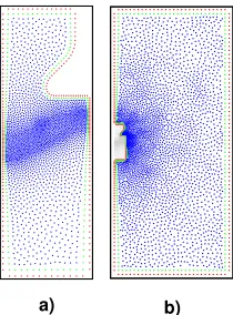
The computational node arrangement (CNA) is unstructured and has variable density of the nodes. A smaller computational domain is used to solve the conservation equations, while a larger one is used to solve the EMF model (see Fig. 4). The number of the nodes is increased in the mushy zone and in the coil area and decreased in the solid phase and at the outer boundary of the EMF domain. The mushy zone is not constant with time, which means that the CNA is adapted on demand. This does not need any additional interference of the user, since an automatic node generation is used in the model.
a) b)
Fig. 4. The computational node arrangement used to solve; a) the conservation and b) EMF equations; The node density is decreased for better visibility
5.3 Point Automata Method
Point automata (PA) method [24] is used for the
simulation of nucleation and grain growth. In
the PA method, the randomly distributed points are used instead of square cells like in the classical
cellular automata (CA) method [25]. Each point has
a defined neighbourhood containing Nneigh nearest
points. Similar as in the CA method, the possible states of the point and the rules for transition between states have to be determined. Each point has three possible states: solid (S), liquid (L), and interface (I). To each point, the concentration in the solid and in the liquid phase for each alloying element and the solid fraction are assigned. The time-dependent temperature and the concentrations in the liquid phase, obtained
Fig. 5.Representation of the solid-liquid interface by PA method; five points inside the dashed line represent the neighbourhood of a point marked with black circle
from the thermofluid model, are assumed to be uniform in the computational domain. At the beginning of
the simulation, stateLand concentrationsC=C0are
assigned to each point in the computational domain. At each time step, all the points in the computational domain are checked.
Nucleation is described by the state L being
changed toIif:
R<Vp
∆T+δ∆T
∆T
dn
d∆Td∆T, (28) whereR∈[0,1).
To describe solidification, stateIis changed toS
ifgs=1. When the state Iis changed to the state S
in a point, the neighbourhood of that point is checked and the state Lis changed to the stateIin all liquid neighbours.
Melting is described by stateIbeing changed to
Lifgs=0. When the stateIis changed to the stateL in a point, the neighbourhood of that point is checked
and the state Sis changed to the stateI in all solid
neighbours.
5.3.1 Calculation of Solid Fraction and Concentration
By assuming the uniform concentration on the scale of a point in the stateI, the lever rule can be written for each alloying element [26]:
Ci+δCi=1+g
s(ki0−1)(Cli∗+δCli∗), (29)
where δ represents a change of a variable during
one explicit time step. Eq. (29) for each alloying element together with Eq. (24) yield a system of
Nalloy+1 equations, which are solved by the use of LU
decomposition in order to obtain δC∗
l andgs in each
point in the state I. TemperatureT∗in Eq. (24) and
δCi are obtained from the thermofluid model. n∗and
κ in Eq. (24) are calculated according to the modified
6 EXPERIMENTAL VALIDATION
The verification of the simulation system has been done by a spectrum of solidification related benchmark tests of which several have been originally proposed
by our group [10] and [19]. The validation
of the simulation system follows a complicated interconnected plant and laboratory measurements
strategy. The plant measurements include: the
electromagnetic field measurements by insertion of the measuring coil in the empty mould; the temperature measurements by insertion of the thermocouples in the melt (see Figs. 6 and 7); measurements of the sump depth by insertion of a steel rod during operation (Fig. 8); the flooding of the sump by pure zinc and then cutting the strand (Fig. 9); measurement of the direct-chill water temperature increase; macrosegregation evaluation by point chemical analysis along the cross section;
measurement of the strand deformation. The
microstructure model is validated by comparison of the calculated and laboratory measured grain sizes and microsegregation.
Fig. 6. Billet instrumented with thermocouples for temperature measurement
6.1 Temperature Measurements
The temperature measurements have been performed with the K type thermocouples, which were inserted into the melt at four different locations. First location was at the billet surface, second one at the centre and the other two at the distance of 50 mm from the centreline. All of the locations are just approximate and are determined in detail by slicing of the finished
product. Validation is performed in the sense of
modifying the boundary conditions for heat transfer in the mould and direct-chill area. The results with the modified boundary conditions are in a very good agreement with the temperature measurements (see Fig. 7).
Fig. 7.Comparison of temperature measurement and simulation along the z-axis atr=52mm; simulation A is performed with generic heat transfer boundary conditions [11]; simulation B is performed with the plant-specific boundary conditions
6.2 Sump Depth Measurements
Sump depth measurements have been performed by insertion of a steel rod into the melt at three different
positions - at the centre, at the r/2 and at the
surface of the billet. The measurement procedure is the following: the rod is inserted from the top in the vertical direction until the coherency isotherm is met. Next the rod is held in that position and the distance from the bottom of the rod to the melt level is measured. Fig. 8 shows the comparison between the sump depth measurements and the simulation results. The solidus and the liquidus isolines are shown with the solid and dashed line, respectively. The results show that the simulated sump depth is a good representation of the actual sump depth, especially considering the measurement error and the fact that it is difficult to define the alloy coherency isotherm.
Fig. 8.Comparison of the simulated and measured mushy area
Fig. 9. Flooding of AlCuBiPb (AA2011) sump with zinc, which has approximately 3 times higher density than aluminium; zinc displaced the aluminium alloy and the position of liquid-solid interphase region is clearly visible after cutting of the billet
7 RESULTS
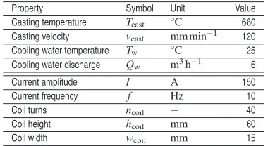
The results presented in this section demonstrate the capabilities of the simulation system and are not meant to be exhaustive. The parameters of the casting process are given in Table 2. The material properties and other required physical parameters are listed in Table 1. The parameters correspond to a typical production configuration of Al-5.25wt%Cu alloy.
Table 1. The material properties of Al-5.25wt%Cu alloy and the steel support structure used in the DCC and LFEC simulations
Property Symbol Unit Value Liquid phase specific heat capacity cpl Jkg−1K−1 1.13×10³
Solid phase specific heat capacity cps Jkg−1K−1 1.03×10³
Liquid phase thermal conductivity kl Wm−1K−1 80.0 Solid phase thermal conductivity ks Wm−1K−1 180
Liquid species diffusivity Di
l m2s−1 0
Solid species diffusivity Di
s m2s−1 0
Density ρ kgm−3 2.6×10³
Dynamic viscosity µ kgm−1s−1 1.40×10⁻³
Gravity acceleration gacc ms−2 9.81
Secondary dendrite arm spacing das µm 25.0 Latent heat Lf Jkg−1 3.77×10⁵
Fusion temperature Tf ◦C 660
Eutectic temperature Te ◦C 548
Eutectic concentration Ce wt% 32.60
Liquidus slope ml ◦Cwt%−1 −3.43
Partition coefficient k0 − 0.173 Thermal expansion coefficient βT K−1 1.17×10⁻⁴
Solutal expansion coefficient βC wt%−1 −7.3×10⁻³
Reference temperature Tref ◦C 700
Reference concentration Cref wt% 5.25
Steel electrical conductivity σSteel Sm−1 1.7×10⁶
Liquid phase electrical conductivity σAl,l Sm−1 4.00×10⁶
Solid phase electrical conductivity σAl,s Sm−1 8.00×10⁶
Stand. dev. of normal dist. ∆Tσ K 6.5 Mean value of normal dist. ∆Tµ K 0.75 Maximal nucleation density nmax m−2 5.5×10¹¹
7.1 Thermofluid
Results of the thermofluid model are summed up in Figs. 10 and 11. The results include the temperature contours for DCC (Fig. 10a), the concentration contours for DCC (Fig. 10b), the velocity magnitude contours with streamlines for DCC (Fig. 11a), and the velocity magnitude contours with streamlines for the case with EMF (Fig. 11b). The solid lines are used to denote the liquidus and solidus isoline. The results without the EMF are used as input parameters for the microstructure and thermomechanical model.
a) b)
Fig. 10. Results of the thermofluid model; a) temperature field for DCC; b) concentration field for DCC
a) b)
Table 2. Casting parameters for the simulated DCC case; parameters below the double line are the additional parameters used to define the electromagnetic field
Property Symbol Unit Value
Casting temperature Tcast ◦C 680
Casting velocity vcast mmmin−1 120
Cooling water temperature Tw ◦C 25
Cooling water discharge Qw m3h−1 6
Current amplitude I A 150
Current frequency f Hz 10
Coil turns ncoil − 40
Coil height hcoil mm 60
Coil width wcoil mm 15
7.2 Microstructure Evolution
The results of the microstructure model are represented in Figs. 12 and 13. The microsegregation and ASTM index can be predicted. The final microstructure in a sample with dimensions 3mm×3mm at the center of the billet is given in the Fig. 12. Corresponding concentration field of Cu is shown in Fig. 13. The microsegregation with increasing concentration of the copper as a function of the radius of a grain is observed.
Fig. 12.Results of the microstructure evolution model: grain structure
Fig. 13. Results of the microstructure evolution model: rescaled concentration field of Cu
7.3 Thermomechanics
The results of thermomechanical model adjacent to the thermofluid model are represented in Figs. 14 and 15. The primary outputs of the mechanical model are the deformation field and the plastic strain field. The magnitude of the latter is shown in Fig. 14a, while Fig. 14b shows the hoop stress obtained from the deformation field. The primary results are combined by models described in Section 3 to predict formation of casting defects. The thermomechanical model can predict the size of the porosity, shown in Fig. 15a, and the susceptibility to hot-tearing, shown in Fig. 15b.
a) b)
Fig. 14.Illustration of results of thermomechanical model; a) plastic strain magnitude; b) hoop stress in Pa
a) b)
Fig. 15. Illustration of prediction of casting defects; a) predicted size of voids inµm; b) hot-tearing susceptibility according to SKK criterion
8 CONCLUSIONS AND OUTLOOK
The presented numerical model of DCC provides additional insight in the DCC process and gives plant
operators options to virtually experiment with the casting parameters to investigate the relations between the casting parameters and presence of chemical and mechanical defects in the produced ingots.
The presented simulation system is unique in the sense that it couples the electromagnetic phenomena with the thermofluid and solid mechanics phenomena
on the macroscopic levels (∼1 m) with the phenomena
on the micro-scale (∼0.1 mm), which has not been
demonstrated before.
The described models are in the process of further improvement. The thermofluid model will be improved by Eulerian-Eulerian description of the grain movement of the solid phase, the microstructure model
will obtain another scale (∼ 0.001 mm) for solving
the detailed shape and structure of the dendrites and its primary and secondary spacing. This scale will be resolved by the phase-field formulation. The solid mechanics level will be improved by replacing the current solution procedure with the state-of-the art return-mapping algorithms, which will allow more complicated constitutive equations to be added to better describe the behaviour of the mushy zone.
The simulation output of all the models will be validated on typical aluminium alloy compositions
from the 1000 to 8000 series. The validation
will proceed with additional plant and laboratory measurements, to improve the nucleation model in particular.
Additionally, the model will be extended to describe three dimensional geometry of slab casting. Such simulations result in computational times on the order of few days on shared-memory computers, requiring supercomputer implementation to achieve reasonable computational times. The computational time will be further reduced by extensive use of automatic adaptive node refinement and coarsening.
To help with validation of the models, we plan to establish a water model of the DCC as already performed for continuous casting of steel [28].
The system will be further improved in the sense of user-friendliness by establishment of alloy specific quality, productivity, and safety object functions as well as automatic searching for the best casting parameters, based on evolutionary computing.
9 NOMENCLATURE
∗ Value at the solid-liquid interface, [-]
α(T) Temperature dependent coefficient of thermal
expansion, [1/K]
α∆t Ratio between time steps at different scales, [-]
βC Solutal expansion coefficient, [-]
βT Thermal expansion coefficient, [1/K]
fg Gravitational force, [N/m3]
t Traction, [Pa]
∆T Undercooling, [K]
∆Tµ Mean of the normal distribution, [K]
∆Tσ Standard deviation of the normal distribution,
[K]
δ Skin depth, [-]
ε4 Strength of anisotropy, [-]
Γ Gibbs-Thomson coefficient, [Km]
γs Surface tension, [N/m]
κ Curvature of the solid-liquid interface, [1/m]
λ Lamé parameter, [Pa]
Ci
kk Intrinsic average concentration of phasek, [-] hkk Intrinsic average enthalpy of phasek, [J/kg] pkk Intrinsic average pressure of phasek, [N/m2] vkk Intrinsic average velocity of phasek, [m/s]
bEM Lorentz force, [N/m3]
g Gravitational acceleration, [m2/s]
R Random number, [-]
τ Octahedral stressτ=σ−Itrσ/3, [Pa]
εe Elastic strain, [-]
εp Plastic strain, [-]
εt Thermal strain, [-]
I Identity tensor, [-]
µ0 Magnetic permeability of vacuum, [H/m]
µl Dynamic viscosity, [kg/(m·s)]
ρ Density, [kg/m3]
σ Electrical conductivity, [S/m]
σe Effective stressσe=
2τ:τ/3, [Pa] σo,σ0 Reference stress, [Pa]
σmax Maximal principal stress, [Pa]
σSKK Critical stress according to SKK criterion, [Pa]
A0 Magnetic vector potential, amplitude, [Vs/m]
B0 Magnetic field, amplitude, [T]
C Array of concentrations, [-]
C0 Array of initial concentrations, [-]
Cl Array of concentrations in the liquid phase, [-]
J0,ext External electric current density, amplitude,
[A/m2]
n∗ Normal to the solid-liquid interface, [-]
v∗ Solid-liquid interface velocity, [m/s]
A,A Reference strain rate, [1/s]
Ci
0 Initial concentration of the i-th alloying
element, [-]
Ci
k Concentration of thei-th alloying element in
thek-th phase, [-]
Ci
ref Reference concentration of the i-th alloying
element, [-]
Ci
m Volume-averaged concentration, [-]
cpk Specific heat capacity of phasek, [J/(kg·K)]
das Secondary dendrite arm spacing, [m]
dg Grain size, [m]
Di
k Diffusion coefficient of the i-th alloying
element in thek-th phase, [m2/s]
E Young’s modulus, [Pa]
fa Anisotropy function, [-]
G Shear modulus, [Pa]
gk Volume fraction of phasek, [-]
href Reference enthalpy, [J/kg]
hm Volume-averaged enthalpy, [J/kg]
hPA Average spacing between neighbouring points
in PA, [m]
k Thermal conductivity, [W/(m·K)]
K0 Permeability constant, [m2]
ki
0 Partition coefficients of the i-th alloying
element, [-]
l Liquid phase, [-]
Lf Latent heat, [J/kg]
Lx,Ly Side lengths of rectangular computational
domain for PA, [m]
mi
l Liquidus slope of the i-th alloying element,
[K]
n Nucleation density, [1/m3]
Nalloy Number of alloying elements, [-]
nmax Maximal nucleation density, [1/m3]
Nneigh Number of neighbours, [-]
p,p Garafalo law exponent, [-]
Q Activation energy of viscoplastic deformation,
[kJ/kg]
R General gas constant, [-]
rp Packing ratio, [-]
s Solid phase, [-]
T Temperature, [K]
t Time, [s]
Tref Reference temperature, [K]
Te Eutectic temperature, [K]
Tf Fusion temperature, [K]
Tl Liquidus temperature, [K]
Ts Solidus temperature, [K]
Vp Volume, represented by one point, [-]
I Interface PA state, [-]
L Liquid PA state, [-]
S Solid PA state, [-]
ACKNOWLEDGEMENTS
This work was supported by the Slovenian Research Agency (J2-7384 Advanced modelling and simulation of liquid-solid processes with free boundaries; L2-6775 Simulation of industrial solidification processes under influence of electromagnetic fields;
P2-0162 Transient two-phase flows); European
Structural and Investment Funds and Slovenian Ministry of Education, Science and Sport (20.00369 MARTINA; 20.03531 MARTIN).
REFERENCES
[1] Eskin, D. G. (2008). Physical Metallurgy of Direct Chill Casting of Aluminum Alloys. CRC Press, Boca Raton, 1 edition edn.
[2] Vertnik, R., Založnik, M., Šarler, B. (2006). Solution of transient direct-chill aluminium billet casting problem with simultaneous material and interphase moving boundaries by a meshless method. Engineering Analysis with Boundary Elements, vol. 30, no. 10, p. 847–855, DOI:10.1016/j.enganabound.2006.05.004. [3] Saunders, N., Guo, U. K. Z., Li, X., Miodownik, A. P.,
Schillé, J.-P. (2003). Using JMatPro to model materials properties and behavior.JOM, vol. 55, no. 12, p. 60–65. [4] Ganesan, S., Poirier, D. R. (1990). Conservation of mass and momentum for the flow of interdendritic liquid during solidification.Metallurgical Transactions B, vol. 21, no. 1, p. 173–181, DOI:10.1007/BF02658128. [5] Poirier, D. R., Nandapurkar, P. J., Ganesan, S. (1991).
The energy and solute conservation equations for dendritic solidification. Metallurgical Transactions B, vol. 22, no. 6, p. 889–900, DOI:10.1007/BF02651165. [6] Ni, J., Beckermann, C. (1991). A volume-averaged
two-phase model for transport phenomena during solidification. Metallurgical Transactions B, vol. 22, no. 3, p. 349–361, DOI:10.1007/BF02651234. [7] Kozeny, J. (1927). ˝Uber kapillare Leitung des Wassers
im Boden. Sitzungsber Akad. Wiss., Wien, vol. 136, no. 2a, p. 271–306.
[8] Chorin, A. (1967). A Numerical Method for Solving Incompressible Viscous Flow Problems. Journal of Computational Physics, vol. 2, no. 1, p. 12–26, DOI:10.
1006/jcph.1997.5716.
[9] Chorin, A. J. (1968). The numerical solution of the Navier-Stokes equations. Mathematics of Computation, vol. 22, no. 104, p. 745–762, DOI:10.
1090/S0002-9904-1967-11853-6.
[10] Hati´c, V., Mavriˇc, B., Šarler, B. (2018). Simulation of a macrosegregation benchmark with a meshless diffuse approximate method. International Journal of Numerical Methods for Heat & Fluid Flow, vol. 28, no. 2, p. 361–380, DOI:10.1108/HFF-04-2017-0143. [11] Weckman, D. C., Niessen, P. (1982). A numerical
simulation of the D.C. continuous casting process including nucleate boiling heat transfer. Metallurgical
Transactions B, vol. 13, no. 4, p. 593–602, DOI:10.
1007/BF02650017.
[12] Kumar, A., Tyagi, M., Specht, E., Bertram, A. (2011). Thermomechanical simulation of direct chill casting.
Transactions of The Indian Institute of Metals, vol. 64, no. 1, p. 13–19.
[13] Suyitno, Kool, W., Katgerman, L. (2009). Integrated Approach for Prediction of Hot Tearing. Metallurgical and Materials Transactions A, vol. 40, no. 10, p. 2388–2400, DOI:10.1007/s11661-009-9941-y. [14] Dantzig, J., Rappaz, M. (2009). Solidification.
Engineering Sciences. EPFL Press.
[15] Liu, G. (2009). Mesh Free Methods: Moving Beyond the Finite Element Method. CRC Press, Boca Raton, FL.
[16] Sadat, H., Prax, C. (1996). Application of the diffuse approximation for solving fluid flow and heat transfer problems. International Journal of Heat and Mass Transfer, vol. 39, no. 1, p. 214–218, DOI:10.1016/
S0017-9310(96)85018-6.
[17] Bertrand, O., Binet, B., Combeau, H., Couturier, S., Delannoy, Y., Gobin, D., Lacroix, M., Le Quéré, P., Médale, M., Mencinger, J., Sadat, H., Vieira, G. (1999). Melting driven by natural convection A comparison exercise: first results.International Journal of Thermal Sciences, vol. 38, no. 1, p. 5–26, DOI:10.
1016/S0035-3159(99)80013-0.
[18] Talat, N., Mavriˇc, B., Belšak, G., Hati´c, V., Bajt, S., Šarler, B. (2018). Development of meshless phase field method for two-phase flow. International Journal of Multiphase Flow, vol. 108, p. 169–180, DOI:10.1016/
j.ijmultiphaseflow.2018.06.003.
[19] Hati´c, V., Cisternas Fernandez, M., Mavriˇc, B., Založnik, M., Combeau, H., Šarler, B. (2019). Simulation of a macrosegregation benchmark in a cylindrical coordinate system with a meshless method.
International Journal of Thermal Sciences, vol. 142, p. 121–133, DOI:10.1016/j.ijthermalsci.2019.04.009. [20] Šarler, B., Vertnik, R. (2006). Meshfree explicit local
radial basis function collocation method for diffusion problems.Computers & Mathematics with Applications, vol. 51, no. 8, p. 1269–1282, DOI:10.1016/j.camwa. 2006.04.013.
[21] Mramor, K., Vertnik, R., Šarler, B. (2013). Low and intermediate Re solution of lid driven cavity problem by local radial basis function collocation method.
Computers, Materials & Continua, vol. 36, no. 1, p. 1–21.
[22] Mavriˇc, B., Šarler, B. (2015). Local radial basis function collocation method for linear thermoelasticity in two dimensions. International Journal of Numerical Methods for Heat & Fluid Flow, vol. 25, no. 6, p. 1488–1510, DOI:10.1108/HFF-11-2014-0359. [23] Hanoglu, U., Šarler, B. (2019). Hot Rolling Simulation
System for Steel Based on Advanced Meshless Solution. Metals, vol. 9, no. 7, p. 788, DOI:10.3390/
met9070788.
[24] Lorbiecka, A. Z., Sarler, B. (2010). Simulation of Dendritic Growth with Different Orientation by Using the Point Automata Method.CMC: Computers, Materials & Continua, vol. 18, no. 1, p. 69–104, DOI:10.3970/cmc.
2010.018.069.
[25] Gandin, C. A., Rappaz, M. (1994). A coupled finite element-cellular automaton model for the prediction of dendritic grain structures in solidification processes.
Acta Metallurgica et Materialia, vol. 42, no. 7, p. 2233–2246, DOI:10.1016/0956-7151(94)90302-6. [26] Jacot, A., Rappaz, M. (2002). A pseudo-front
tracking technique for the modelling of solidification microstructures in multi-component alloys. Acta Materialia, vol. 50, no. 8, p. 1909–1926, DOI:10.1016/
S1359-6454(01)00442-6.
[27] Raabe, D., Roters, F., Barlat, F., Chen, L.-Q., editors (2004). Continuum Scale Simulation of Engineering Materials: Fundamentals - Microstructures - Process Applications. Wiley-VCH, Weinheim, 1 edition edn. [28] Gregorc, J., Šarler, B. (2018). Experimental research