in the population sciences published by the Max Planck Institute for Demographic Research Konrad-Zuse Str. 1, D-18057 Rostock·GERMANY www.demographic-research.org
DEMOGRAPHIC RESEARCH
VOLUME 17, ARTICLE 4, PAGES 83-108
PUBLISHED 17 AUGUST 2007
http://www.demographic-research.org/Volumes/Vol17/4/ DOI: 10.4054/DemRes.2007.17.4
Research Article
Differential mortality by lifetime earnings
in Germany
Hans-Martin von Gaudecker
Rembrandt D. Scholz
c
2007 von Gaudecker & Scholz
1 Introduction 84
2 Data and methodology 85
2.1 The German public pension system 85
2.2 Description of the dataset 88
2.3 Methods and terminology 90
3 Results 91
3.1 Mortality rates for selected earnings points groups 92
3.2 Period life expectancies at age 65 by EPpers 92
3.3 Mortality by EPpersand EPCP 95
3.4 Life expectancy at age 65 by EPpersand place of residence 97
3.5 International comparisons 101
4 Conclusions 102
5 Acknowledgements 103
References 104
Differential mortality by lifetime earnings in Germany
Hans-Martin von Gaudecker1
Rembrandt D. Scholz2
Abstract
We estimate mortality rates by a measure of socio-economic status in a very large sam-ple of male German pensioners aged 65 or older. Our analysis is entirely nonparametric. Furthermore, the data enable us to compare mortality experiences in eastern and western Germany conditional on socio-economic status. As a simple summary measure, we com-pute period life expectancies at age 65. Our findings show a lower bound of almost 50 percent (six years) on the difference in life expectancy between the lowest and the highest socio-economic group considered. Within groups, we find similar values for the former GDR and western Germany. Our analysis contributes to the literature in three aspects. First, we provide the first population-based differential mortality study for Germany. Sec-ond, we use a novel measure of lifetime earnings as a proxy for socio-economic status that remains applicable to retired people. Third, the comparison between eastern and western Germany may provide some interesting insights for transformation countries.
1Free University Amsterdam, Department of Economics, De Boelelaan 1105, 1081 HV Amsterdam, The
Netherlands, E-mail: [email protected]
2Rostocker Zentrum zur Erforschung des Demografischen Wandels, Germany. E-mail:
1.
Introduction
The international literature on socio-economic status and mortality is marked by a per-sisting absence of studies on Germany,3 probably owing to the lack of large high
qual-ity datasets. Fortunately, the situation has changed since the inception of the Research Data Centre of the German Pension Insurance (Forschungsdatenzentrum der Rentenver-sicherung) which has made available a large database of public pension records. These data enable us to make a number of, albeit small, contributions to the existing literature.
We document mortality inequalities among elderly men in Germany. The data permit us to compare the regions of the former German Democratic Republic (GDR) with the rest of Germany. Due to the very different institutions for forty years, differences may well be expected. In addition, the German pension system enables us to measure socio-economic status by means of a variable which we term lifetime earnings, a discounted sum of pensionable earnings over the life-cycle. We argue that the variable is a very broad measure of socio-economic status that is also readily applicable to the retired population. Finally, due to the large size of our dataset, we do not need to resort to any parametric assumptions on the structure of the relationship between lifetime earnings and mortality.4 For period life expectancy at age 65, our results indicate a lower bound of six years on the difference between the lowest and the highest earnings group considered in our study. As measured from the lowest group, this constitutes a difference of almost fifty percent. Life expectancy rises almost linearly over a sizable part of the lifetime earnings distribution. Despite the fact that we do find lower overall mortality in western Germany than in the former GDR, our results show similar life expectancies within income groups. The unconditional difference, hence, comes from composition effects.
Our results merely reveal a correlation between lifetime earnings and mortality. From our estimates, nothing can be said about the underlying pathways that lead to these figures. In general, three broad channels of causality can be imagined. Epidemiologists stress the importance of causality from income to health (Marmot, 1999). Economists are often preoccupied with quantifying the reverse direction by which it is a low health status that impairs current and future earnings capacity (Smith, 2004). A third explanation is that there are one or more underlying factors determining both income and health. Among many potential candidates are genetics, ability, intelligence, social skills, networks, and other background or early life factors, such as parental income (Case et al. 2002) or education (Lleras Muney, 2005). We see our contribution in documenting a strong re-lationship between lifetime earnings and life expectancy in Germany that calls for more research on its origins.
The structure of this paper is as follows. We first describe the data in Section 2, with particular emphasis on the German pension system and the calculation of the central explanatory variable. Section 3 contains the presentation of our results in three stages, followed by some international comparisons. Finally, a conclusion is provided in Sec-tion 4.
2.
Data and methodology
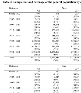
We use a very large dataset of administrative records from the German Public Pension System. For reasons explained in Section 2.2, we consider only male individuals. Our data cover more than 80 percent of the whole male population born in 1936 or earlier. Consider the first and fifth column of Table 2 in the Appendix on page 107. They show our sample sizes and the fractions of the general population covered by our data broken down by age group and region of residence. Coverage is about three quarters in western Germany, but it drops substantially to less than two thirds at older ages. This is likely to be due to differential mortality since people outside the system tend to have a higher socio-economic status. In terms of selection bias, we do not see any reason why results on differential mortality among the pensioners covered by our data should not extend qualitatively to the rest of the population. Coverage rates in the eastern region are higher, reaching up to 98 percent. This is because in the former GDR, virtually everyone was in-sured under the state pension system. At the same time there were exceptions for the self-employed and civil servants (see Section 2.1) in the Federal Republic of Germany (FRG) that explain the baseline difference.
In the next section, we turn to the derivation of the central variable of our analysis, an internal measure of the Public Pension System used to calculate pension benefits (personal earnings points). It serves reasonably well as an indicator of total lifetime earnings. Sec-tion 2.2 presents the descriptive statistics of the variables used in our analysis and deals with the creation of our dataset from several sources of administrative records. Finally, in Section 2.3 we turn to our estimation methods.
2.1 The German public pension system
The German Public Pension System in the form that is relevant for the cohorts studied in this analysis is a pay-as-you-go system based on a single tier. Benefits are directly related to personal earnings over the life-cycle.5This section provides a very brief introduction to
those parts of the system that are relevant for the purposes of the paper. Our description is based on Börsch-Supan and Wilke (2004) and VDR (2004). The system covers all private
and public sector employees. It excludes civil servants (about 7 percent of the workforce) and most self-employed (about 9 percent). The latter can voluntarily insure themselves in the system; we will get back to this in Section 2.2. Our focus is on old-age pensions, paid to all retirees age 65 and above. By the end of the calender year in which age 65 is reached, almost everyone is retired in the sense that he claims pension benefits.6 7
Key to the system are the so-called earnings points, which essentially are a measure of the relative annual earnings position. In any given yeart, the earnings points for con-tribution periods (EPCP) of an individualiare calculated as:
EPCPit =
pensionable earningsit
average pensionable earningst (1)
In 2002, pensionable earnings were the first 4,500 Euro of gross monthly earnings if the they were above the minimum earnings threshold of 325 Euro. A subset of our data contains the sum of EPCPit over alltwith relevant contributions for each individual (we call this variable EPCPi ). Note that this variable is subject to right censoring because of the annual upper limit to pensionable income. Hence, we know only a lower bound for the earnings of people with high EPCPi . This has to be kept in mind when interpreting the results. By contrast, the left censoring at 325 Euro is negligible. We note that because of the division by average pensionable earnings in (1), the discount rate inherent to EPCPi is
the annual growth rate of average pensionable earnings.
For administrative reasons, EPCPi is available only for individuals who retired after a
major reform to the system in 1992. The measure recorded for all persons in our dataset is called personal earnings points (EPpers). These are calculated as follows:
EPpersi = (EPCPi +EP N CP
i )·AFi (2)
EPN CP stands for earnings points from non-contributory periods. These stem from spells
with no contributions at all which are nonetheless relevant for pension benefits. They in-clude, for example, long-term sickness or unemployment spells, the months during which disability pensions were received,8 some allowance for advanced education, and so on.
The adjustment factor AFi scales down earnings points in the case of early retirement
after the 1992 reform. For the purpose of our analysis it also serves to capture a type of
6It is virtually impossible to remain in paid employment while receiving pension benefits because of very low
earnings thresholds. Hence this is almost identical to defining retirement as not participating in the labour force.
7For the 1936 cohort (the youngest cohort in our analysis), internal statistics of the Deutsche Rentenversicherung
show that only 0.56 percent were not retired on 1st January 2002, the starting point of our analysis.
8Legislation on disability pensions has been subject to several reforms over the years. They are paid until age 65
minimum pension benefit for low earnings (Mindestentgeltpunkte bei geringem Arbeit-sentgelt) that was effective until 1992.
Individual pension payments are obtained directly from EPpersi by multiplication with the current pension value common for all pensioners. In 2002 it was 25.86 Euro for EPpersi earned in the FRG and 22.97 Euro for those EPpersi earned in the GDR. For example, 50 EPperstranslate into a monthly gross pension payment of 1293.00 Euro if all EPpers were earned in the FRG. The current pension value is adjusted annually according to complex procedures. This does not impact our analysis, however. We only need the fact that EPCP and EPpers remain constant once an individual receives an old-age pension. There are some minor qualifications for EPpers, for example due to divorce or moving abroad. Since we only include pensioners living in Germany (see Section 2.2), the latter does not impact our analysis and we treat the former as negligible.9
We prefer EPCPas a measure of lifetime earnings because EPperscontains too many
items that have nothing to do with lifetime earnings but rather reflect social policy mea-sures. For cohorts born after 1928, we can compare both meamea-sures. Correlations are very high withρ '0.95. We present the results of a comparative analysis of mortality experiences based on the two different measures in Section 3.3. Our results show that the distinction is not all too important in terms of describing the mortality experience by earnings group for ages 65 to 73. For the calculation of life expectancies we also need the mortality experience of older cohorts. Hence, we extrapolate the similarity re-sult and interpret EPpers as lifetime earnings, although there is larger error inherent to EPpersthan to EPCP . The nice feature of these variables is that they give us a measure of long-run earnings. This is a much better measure for socio-economic status than current income typically recorded in surveys. The latter is often blurred by transitory fluctua-tions, which are surprisingly high. These may lead to serious biases as documented in Haider and Solon (2006). Our discounted sum of lifetime earnings misses out on some things typically included in the income definition (for example, bequests, capital income or transfers). Bearing the incompleteness in mind, we use lifetime earnings and lifetime income as synonyms in the remainder of the paper. Another large advantage of the mea-sure is that it remains applicable to retired persons; using broader meamea-sures may lead to biases due to differences in savings behaviour at earlier stages of the life-cycle.
The description of the pension system has focused on the (western) FRG until 1990 and the (unified) FRG thereafter. In the GDR, there was a somewhat different system at work. It is beyond the scope of this paper to provide a detailed description of this system but we note that accumulated earnings points are comparable in the sense that GDR earnings points are also based on the length of the work life and the position in
9Calculations based on the “Versorgungsausgleichstatistik” show that changes in EPpersdue to divorce affect
the annual earnings distribution. A detailed description of how pension entitlements were transferred is contained in Stephan (1999). It is safe to say that the amount of income needed to gain one earnings point in the GDR had much less buying power than the amount of income needed to gain one earnings point in the FRG. However, the pension income that derives from GDR earnings points is only 13 percent less than the one based on FRG earnings points. Hence the relative position in the earnings distribution and pension income streams are comparable while economic status during the working life is not.
Let us close this section with a brief illustration of the monthly pensionable income necessary to accumulate a certain amount of earnings points. In 2002, the monthly gross earnings that yielded one EPpers was about 2,400 Euro. For simplicity, assume that
this number remains constant over an individual’s working life. Hence, to accumulate 50 EPpers, a person with this earnings would have to work 50 years. If average monthly
earnings over the life-cycle were 3,000 Euro, 40 full years of contribution would be suffi-cient to accumulate the same amount of EPpers.
2.2 Description of the dataset
The administration of the German public pension system is marked by a variety of statu-tory bodies. Traditionally, there have been regional pension insurance bodies for workers, a federal body for salaried employees, and three profession-specific bodies. Except for miners, legal regulations have been the same since 1949. All pension insurance bodies are required by law to report statistics of all pensioners as of the end of each year as well as statistics of those pensioners who died during that year to their umbrella association.10 We have access to these data.11 Because only selective characteristics of the original ad-ministrative records enter our dataset, some important remarks about the structure and peculiarities of the data are in order.
For one thing, there is no way of linking members of the same household. Ideally, we would want to use lifetime household income as a relevant measure to correlate with mortality. However, because of the low female labour force participation in the cohorts relevant to our analysis, we exclude them from the analysis. It simply is unclear what the household income position of women with low EPCP is because of the dominance of
male earnings in total household income.
10This used to be the Verband Deutscher Rentenversicherungsträger (VDR). After a major organisational reform
that took effect on 1st October 2005, its duties are now performed by the Deutsche Rentenversicherung Bund, the federal pensions institute.
11Traditionally, only aggregate statistics were published. This has changed since the beginning of 2004 with the
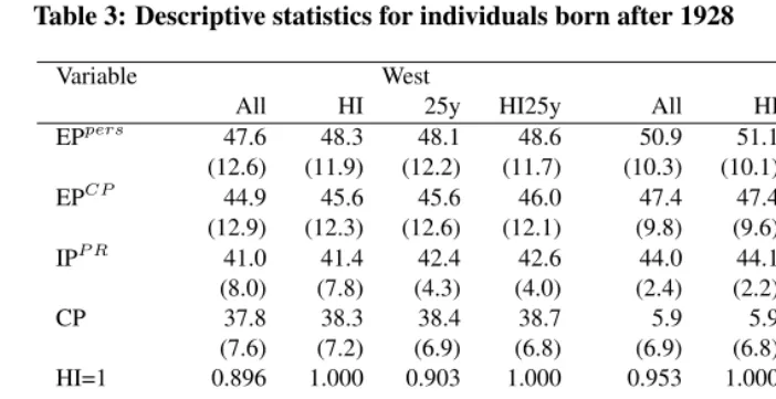
For all individuals in our dataset, we have the year and month of birth. We only use individuals born in 1936 and earlier because of possible health and income differentials in early retirement. Put differently, if we were to use younger pensioners, most likely we would not have a random sample. A further demographic variable is the region of resi-dence in three categories (eastern Germany, western Germany, foreign). We exclude peo-ple with foreign residence (2.3 percent) in order to work with a subset of those recorded in official population statistics. Including them did not cause any visible differences in the mortality estimates. The data contain all deaths in 2002; these are recorded on a monthly basis. The Appendix contains descriptive statistics for the entire sample in Table 1. Those restricted to pensioners born after 1928 are listed in Table 3.
In terms of variables related to pension payments, the two most important ones are those described in the last section. Note that EPpers is on average about 3.1 points (6.6 percent) higher than EPCP in columns 1 and 5 of Table 3. We also have the cor-responding variables on the length of being insured. These are pension-relevant insurance periods (IPP R) and contribution periods (CP). The former are comprised of the latter and of non-contributory periods leading to pension benefit entitlements (see Section 2.1 for examples). Last, we use information on the type of health insurance coverage. Employees are mandatorily covered by the public mutual funds system up to an earnings threshold that was 75 percent of the maximum pensionable earnings until 2003. Individuals above that threshold, the self-employed, and civil servants can either stay voluntarily in the sys-tem or opt out to join a private insurance company. A small subgroup of pensioners in our sample is insured under foreign law, these persons usually worked in Germany only for short periods of time. The arrangement of the last employment spell usually carries over to retirement. We can identify three groups in our data: mandatorily insured; voluntarily or privately insured; insured under foreign law.
The reason why this assumes importance lies in work biographies that are not confined to a single system of pension insurance. To provide an example, take somebody who is employed for ten years and then becomes a civil servant for the rest of his working life. If we used EPCP as a measure of his lifetime earnings, we would make a severe error
in Section 3.2) and because there are more missing values at old ages. The only variable that is completely available is EPpers because it is central to the pension payment. In
conversations with statisticians at the Deutsche Rentenversicherung Bund, we tried to evaluate the influence of systematic effects on missing values. Except for the cases we mention, there is no reason to expect a missing at random assumption to be violated. In eastern Germany, the picture remains much better with coverage rates above 90 percent except for the very old ages.
There are three more variables available; however we do not consider them in the pre-sentation of differential mortality by lifetime earnings for clarity reasons. The variables in question are citizenship in two categories (German/non-German), whether a pension entitlement for repatriates forms part of the total pension, and whether EPpersincludes a scaling-up of raw earnings points because of low earnings before 1992 (cf. Section 2.1). Confining our analysis to Germans who do not fall into either of the last two categories did not substantially alter any results (tables and graphs are available from the authors upon request).
2.3 Methods and terminology
Throughout the analysis, we divide the sample into eleven equally spaced groups of earn-ings points. We then calculate age-specific mortality rates for each of these groups, using the standard Chiang (1984) formulas. It is useful to relate this procedure of calculating mortality differentials to the typically employed logit model. Our analysis is closest to a logistic regression for mortality rates that utilises as covariates the eleven dummy vari-ables for the earnings points categories, a full set of age dummies, and all interaction terms between the two sets of variables. By virtue of the large amount of data, we can allow for this very general specification of the relationship between age, lifetime earnings, and mortality. Compared to the logit model, we furthermore relax the distributional assump-tion on the error term. In the logit case, the disturbances are assumed to follow a logistic distribution. If this assumption is incorrect, the estimates may be biased and confidence intervals are too narrow. In the sense that we do not invoke any distributional assump-tion on the error term, our model is entirely nonparametric (see Schmertmann (1995) for an introduction of nonparametric regression techniques and terminology in demographic research). The typical justification for highly parameterised models as the logit lies in efficiency gains relative to more general techniques. Again, it is the large sample size that allows us to get by without these potentially restrictive assumptions.
period life expectancies. These constitute the main statistic we use to conduct the analysis. Note that the term “life expectancy” might lead to some confusion because its everyday use differs from its scientific content. The period life expectancies that we calculate do notreflect actual life expectancies of any individual in our dataset or elsewhere. Rather, they are a weighted average of 39 age-specific mortality rates that are calculated on the basis of as many different cohorts. Life expectancies in our sense are simply a means of comparing mortality experiences across different population segments, aggregating out the age dimension. This confusion of terms applies to any period life expectancy. For example, a statement like “[...] today, the longest expectation of life – almost 85 years – is enjoyed by Japanese women.” (Oeppen and Vaupel, 2002) does not reflect the life expectancy by any individual female Japanese in 2002. In our case, a typical sentence may read “In the group with 60-64 EPpers, remaining life expectancy is 16.88 years”, however the number does not reflect the life expectancy of any individual in our sample, it merely serves to compare mortality experiences of differences of different subgroups. At some points, we will calculate another statistic based on the mortality rates, namely the probability to reach age 74 by earnings points category. Exactly the same comments on the interpretation of the numbers apply also here – this does not constitute the relevant probability for any real individual.
3.
Results
Our analysis is motivated by time series evidence of rising per-capita pension payments over time within cohorts. Net of changes to the current pension value (see Section 2.1 for details), this can only be due to changes in cohort composition. Once everyone is retired, differential mortality is the sole reason for this phenomenon to occur, i.e. persons with less than average EPpersare dying relatively more frequently than those with higher
3.1 Mortality rates for selected earnings points groups
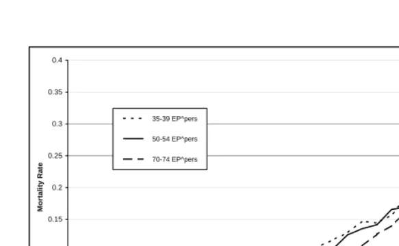
Figure 1 shows the mortality rates for selected groups of EPpers. We refrained from
showing all eleven income classes for legibility reasons. Mortality rates were calculated separately for each one-year age band. The most salient feature of the graph is that the shape of the three curves is very similar, they seem to differ by little more than a parallel shift until sample sizes become very small at advanced ages.12 The similarity in shapes
and particularly the fact that the curves are not crossing (except at very high ages) show that it is feasible to aggregate out the age dimension to compare mortality experiences in a more parsimonious fashion. Confidence bands for each age are not shown in order to keep the graphs readable. They show that until age 76, all three are statistically different from each other at the 99 percent-level. Mortality rates in the highest income group are significantly lower than the other two even until age 83.
3.2 Period life expectancies at age 65 by EPpers
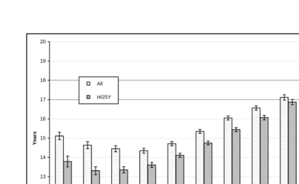
While curves of the type depicted in Figure 1 carry all the information that results from our regression analysis, they are too detailed to provide a basis for overall comparisons. For this reason, we calculate period life expectancies at age 65. All the usual caveats for the interpretation of period life expectancies apply, see Section 2.3 for details. First consider the light bars in Figure 2. They depict e65for the full sample of pensioners we use. Overall remaining life expectancy is at 15.74 years. We postpone a comparison with estimates for the general population to the end of this section. The mortality estimates by earnings points group range from 14.35 years (35-39 EPpers) to 18.65 years (70-74 EPpers). Between these two extremes, life expectancy appears to rise roughly linearly over the groups. Differences among almost all groups are statistically significant at any typical confidence level.
The most striking finding at this very first glance is that minimum life expectancy is reached close to the middle of the table and not in the lowest income group. At the bottom of the distribution, e65is up to more than 15 years again. This stands in contrast to the overwhelming international evidence indicating a monotone and positive relationship between income and life expectancy. Typically, the gradient is found to be steepest in the lower tail (see, for example, Attanasio and Hoynes (2000)). However, there is a plausible reason at hand. As explained in the last section, we expect a very heterogeneous group at the lower end of the distribution because of persons covered by the public pension system
12It is certainly much closer to a parallel shift in mortality than to a parallel shift in log mortality (figures are
Figure 1: Mortality rate by EPpers
0 0.05 0.1 0.15 0.2 0.25 0.3 0.35 0.4
65 70 75 80 85 90 95
Age in Years
M
o
rtal
it
y R
a
te
35-39 EP^pers
50-54 EP^pers
70-74 EP^pers
Note:Only the persons mandatorily enrolled in the public health insurance scheme with at least 25 years of pension-relevant insurance periods are included in the analysis (selection HI25Y).
only during parts of their working life. These are typically well-earning academics who would be at the right tail of the distribution if we observed their full earnings history. To take a colourful example, we would expect to find production line workers next to their company’s CEO in these groups.
A way of shedding light on this issue is to exclude those for whom lifetime earnings are observed with a known systematic error. We try to do so by selecting only those who are mandatorily enrolled in the public mutual funds health insurance system or those who spent at least 25 years in the public pension system. The dark bars in Figure 2 indicate the results when we impose both restrictions. For brevity reasons, we do not present the results if selection is based on one criterion only. Again, the tables are available upon request.
Figure 2: Remaining life expectancy at age 65 in years by EPpers
10 11 12 13 14 15 16 17 18 19 20
20-24 25-29 30-34 35-39 40-44 45-49 50-54 55-59 60-64 65-69 70-74 overall
Earnings Points
Y
ears
All HI25Y
Note:Comparison of all pensioners with the respective amount of EPpersand those who are mandatorily insured in the public health insurance scheme with at least 25 years of pension-relevant insurance periods (HI25Y). The vertical bars indicate 99 percent confidence intervals
decline is particularly pronounced in the lowest income categories. Minimum e65is now 13.31 years for those with 25-29 EPpers, the slight rise for the lowest income category is
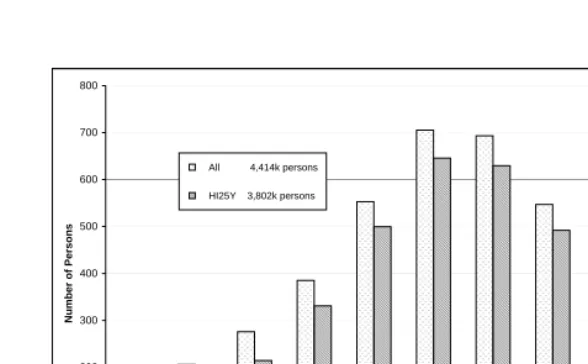
only borderline significant. We suspect this differential drop to be a combination of two effects. On the one hand, the relative size of the sample that is excluded is much higher at lower earnings points levels (57 percent in the lowest category as compared to less than 10 percent in the top seven classes, see Figure 3). On the other hand, if the excluded group is relatively homogeneous, the differential in e65is largest in the lower categories under the hypothesis of a monotonic relationship between income and mortality.
bound on differences in life expectancy is quite substantial. Taking the results from the “HI25Y” selection and the unconditional e65as a starting point, life expectancy of persons in the highest income group is 25 percent higher. On the other hand, if only 25-29 EPpers were accumulated, it is 12 percent lower.
Coming back to the precise relationship between earnings points and life expectancy, we find that it rises almost linearly from the group with 35-39 EPpers to the one with 60-64 EPpers. In this range, neither top-coding nor earnings outside the pension system should be a major cause of measurement error. It is difficult to compare this linearity finding to other studies (see also Section 3.5) since all those that we are aware of either use quantiles of the income/earnings distribution or impose some functional form on the data. While the linear relationship certainly does not extrapolate to larger incomes13this
finding shows the need to allow for flexible functional forms which accommodate (near) linearity on parts of the distribution.
Our results compare quite well with all-population mortality. Official statistics in-dicate a remaining life expectancy at age 65 for German males in 2002 of 16.08 years (HMD, 2006) This is about 4 months higher than our estimates for the full sample in-dicate. In terms of socio-economic status and mortality experience, most of the persons not covered in our data should be roughly comparable to those that were excluded when we imposed the “HI25Y” restriction. Simplifying the matter slightly, the main difference between them is that one group worked for a few years in a job that got them covered by the public pension system and then changed to another one; the other group started in such another job already. Following this argument, we did expect a qualitatively similar rise in life expectancy if we move from “All” to the full population as the one that we see when moving from “HI25Y” to “All”.
3.3 Mortality by EPpersand EPCP
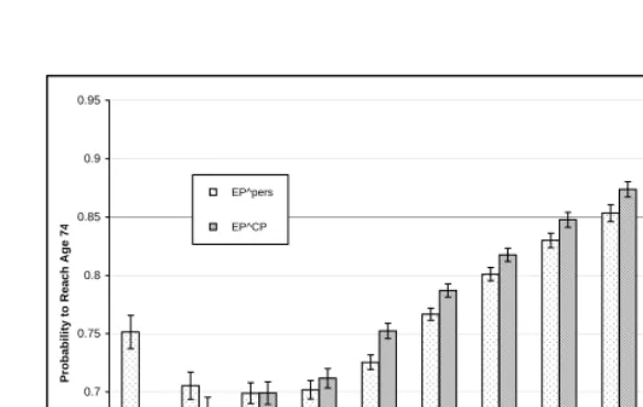
The purpose of this section is to contrast the two different measures of lifetime earnings for those persons where both measures are available (see Section 2.1). These are the cohorts born in 1929 or later because most of them did not retire before 1992. Remaining life expectancy is no longer a suitable summary statistic because we do not have any information on old-age mortality conditional on EPCP. As an alternative, we chose the
probability of reaching age 74 (this is the highest age we can do) conditional on reaching age 65 (P65{74}). The results are shown in Figure 4. The light bars depict P65{74} conditional on EPpers, the dark ones show the corresponding values based on EPCP. The
13To see this, note that if we extrapolated our results one would need to observe e
65= 54years for persons who
Figure 3: The distribution of EPpersby sample selection
0 100 200 300 400 500 600 700 800
20-24 25-29 30-34 35-39 40-44 45-49 50-54 55-59 60-64 65-69 70-74
Earnings Points
Number of Persons
All 4,414k persons HI25Y 3,802k persons
Note:“All” includes all available observations, “HI25Y” incorporates only those mandatorily enrolled in the public health insurance scheme with at least 25 years of pension-relevant insurance periods.
same comments apply to the limited interpretability of these probabilities as to the life expectancies (see Section 2.3).
Overall probabilities are identical at 76.4 percent because we use the same sample in both cases. In the case of EPpers, we find very much the same pattern as for life ex-pectancy in the last section. There is a linear decline from the highest income class to persons with 35-39 EPperswhich then levels out and rises again at the very bottom. The dark bars look quite similar, but there are some important differences. On the one hand, probabilities are slightly higher for all groups with more than 35 EPCP. However, the de-cline does not level out at this point but continues linearly to the very lowest group. Based on this measure, 65-year-old individuals in the highest earnings class have a 90 percent probability of reaching age 74. Less than two thirds in the bottom category survive to this age.
Figure 4: Probability of reaching age 74 at age 65 by EPpers
0.6 0.65 0.7 0.75 0.8 0.85 0.9 0.95
20-24 25-29 30-34 35-39 40-44 45-49 50-54 55-59 60-64 65-69 70-74 overall
Earnings Points
P
roba
bilit
y
t
o
R
each
A
g
e 7
4
EP^pers
EP^CP
Note:Only the persons mandatorily enrolled in the public health insurance scheme with at least 25 years of pension-relevant insurance periods are included in the analysis (selection HI25Y). The vertical bars indicate 99 percent confidence intervals.
than a constant that is mostly explained by the average differential of 3 points between the two measures (see the first two rows of Table 3). On the other hand, the choice of variable does matter in lower categories. By using EPCP as a measure of lifetime earnings, we can reproduce the monotonic relationship to mortality documented in international studies.
In the course of the analyses contained in this section we also checked whether dif-ferences exist if we condition on actual contribution periods (CP) rather than pension-relevant insurance periods (IPP R). One may have expected differences analogous to those resulting from the two earnings measures. However, none such differences became ap-parent which is why we do not include a graph on that point.
3.4 Life expectancy at age 65 by EPpersand place of residence
because of the very different biographies of people living in either region. One could expect several things to happen in the eastern region. There may be a long-run effect of the more equal distribution of socio-economic status during the socialist era, resulting in smaller mortality differentials. The opposite story may read that the sharp transformation in the early 1990s led to higher inequality than in the West. Finally, one may assume relatively fast adaption to the new institutional arrangement, hence a picture that parallels that in the West.14
Naturally, the first thing to evaluate is e65 not stratified by income. We find it to be 15.83 years in western Germany and 15.41 years in the former GDR. The difference is statistically significant at any common confidence level. This compares to full-population estimates from official statistics of 16.19 years and 15.39 years, respectively. In the West we have the effect described above: The 23 percent of the population not included in our sample tend to have a lower mortality than the pensioners. However, the 94 percent cov-erage in eastern Germany leads to almost identical estimates of all-population mortality, so we are very confident to have a complete depiction of the full population there. Our findings are consistent with the converging mortality experiences in both regions that have been documented by several authors (cf. for example Nolte et al. (2000)).
Again, the main analysis concerns the comparison of life expectancy by income group. As in the previous sections, we base selection on mandatory enrollment in a public mu-tual funds health insurance and 25 years of coverage in the pension system. The reason not to consider all-pensioner mortality here is that groups are more comparable in the restricted sample. As discussed in Section 2.2, we expect much more heterogeneity in terms of earnings outside the system in the West than in the East, particularly in the low-est categories. This is because in the former GDR, virtually everyone was insured under the public pension system. Hence, we would obtain a stronger bias within income classes if we did not impose the restrictions. The reason is the larger heterogeneity with respect to socio-economic status in the West. The restriction of the sample makes the analysis within categories more meaningful, but a comparison of unconditional life expectancies does not make much sense. This is clear from the rightmost bars in Figure 5. While e65 does not change for pensioners in the east of Germany, imposing the restriction leads to a drop in remaining life expectancy to 15.14 years in the West. This reversal is due to the
14Migration between the two regions was low and we neglect possible biases in the interpretation of results. Most
Figure 5: Remaining life expectancy at age 65 in years by place of residence and EPpers
10 11 12 13 14 15 16 17 18 19 20
20-24 25-29 30-34 35-39 40-44 45-49 50-54 55-59 60-64 65-69 70-74 overall
Earnings Points
Y
ears
West East
Note:Only the persons mandatorily insured in the public health insurance scheme with at least 25 years of pension-relevant insurance periods are included in the analysis (selection HI25Y). The vertical bars indicate 99 percent confidence intervals.
fact that we excluded a large group of men with high socio-economic status in western Germany and only few persons in the eastern region.
Comparing the graphs for both regions in Figure 5, it becomes apparent that no dif-ference between them can be asserted for groups with more than 40 EPpers. In all groups
com-Figure 6: The distribution of EPpersby place of residence
0% 2% 4% 6% 8% 10% 12% 14% 16% 18% 20%
20-24 25-29 30-34 35-39 40-44 45-49 50-54 55-59 60-64 65-69 70-74
Earnings Points
Relative Number of Persons
West 2,904k persons
East 897k persons
Note:Only the persons mandatorily insured in the public health insurance scheme with at least 25 years of pension-relevant insurance periods are included in the analysis (selection HI25Y).
pared to western Germany under the HI25Y selection, see Figure 6. In other words, there are relatively more people in the higher income classes with a longer life expectancy.
This analysis sheds new light on previous findings from the epidemiological litera-ture. Several authors reported a larger predictive power of income for health measures in western Germany than in the eastern region (Mielck et al. (2000), Nolte and McKee (2004)). Our results suggest this to be a consequence of measurement error, unless the link between morbidity and mortality works differently between both regions. The rel-evant income concept as a marker for socio-economic status is a long-run measure, the surveys employed in the cited studies contain a current income variable. Transitory fluc-tuations, for example due to high unemployment in the East, may well impact strongly upon the analysis. Here we conclude that the inequalities with respect to pension income have the same magnitude in both regions.
rights, comparatively small wage differentials, high job security, an economy with a large amount of goods rationing, etc. People on the other side of the wall experienced much higher wage differentials, somewhat lower job security, a market economy, and quite well protected civil rights. Only from 1990 onwards – the cohorts in our analysis were already at least 53 years old – did institutional arrangements start to converge, although large differences remain, for example in the labour markets. In the light of the observed convergence in total mortality (Nolte, Shkolnikov, and McKee, 2000), we note that this convergence appears to be nearly perfect conditional on our measure of socio-economic status. A natural interpretation of this would be an income effect: Reunification brought about much higher real incomes for pensioners and 12 years were enough to wipe out any lagged effects. Differences in total mortality continue to exist only because of the composition effects – in western Germany there are relatively more persons with a high socio-economic status. Note that it does not follow from this that redistribution would lead to equal mortality experiences – higher pension income in our case is also indicative of a higher ranking in the relative income distribution in the GDR/FRG. The parameters giving rise to this ranking are very likely to be related to mortality, both directly and through interaction effects with income. Examples include education, intelligence, social skills and networks, or genetics. However, if interpreted in this fashion, our results suggest that redistribution would lead to a convergence in mortality experiences among socio-economic groups; the extent of this remains unclear, however.
3.5 International comparisons
In this section, we place our results in the context of the literature on differential mortality. Closest in terms of regional proximity and research question is certainly Reil-Held (2000). She uses survey panel data and finds a life expectancy (e37) differential of 10 years be-tween the top and the bottom quartile of the income distribution, employing a somewhat broader household income variable that is averaged across time. This is in her bivariate analysis that is comparable to our approach. In Reil-Held (2000), the nonparametric anal-ysis serves mainly motivational purposes and confidence intervals are not provided. We obtained her raw estimates and compared the values of e65. Her findings suggest some 17.8 years for the top income quartile and 10.1 years for the bottom one. The slightly lower value for the top quartile may be explained by the earlier time period (she con-sidered deaths in the 1984-1997 period). The much lower value for the bottom quartile is most likely due to our not very meaningful income data for that population segment. Taken together, the numbers compare very well and our claim to have identified a lower bound of 6 years on the life expectancy difference from the bottom to the top is reinforced by her findings of a 7.7 year differential.
status, the study by Huisman et al. (2004) serves well to place our results into a European context. They analyse differential mortality by education and housing tenure and find results that are quite similar to ours in qualitative terms. Throughout the 11 countries included in their study, relative mortality risks declined with age, but absolute mortality differences remained constant or increased until old age. This is exactly what we find from Figure 1. It is not sensible to compare precise numbers because of the differences in covariates. Doblhammer et al. (2005) compare mortality by occupational and educational group in Austria and also find large differences. Again, they report relative mortality risks and the quantities are not easily compared.
Further corroborative evidence for our findings comes from the US – Deaton and Pax-son (2004) report e25to be about 10 years lower for members of families with an annual income of less than $5,000 as compared to those earning more than $50,000. Findings from Attanasio and Hoynes (2000) suggest that the gradient linking income and mortality is steepest at the bottom of the distribution. Since there is no reason to expect this finding to reverse in Germany, this is supportive of our claim that we cannot identify people at the lower end of the distribution very well and mortality conditional on correctly measured income would be much higher. Finally, turning back to Europe, Attanasio and Emmerson (2003) show that the position in the wealth ranking has a large impact on survival proba-bilities in the UK. Palme and Sandgren (2004) are able to construct a measure of lifetime income for a cohort born in 1928 in the city of Malmö, Sweden. They find this variable to be only marginally significant in the case of prime-age mortality. However, their sample size is rather small and they conduct their analyses conditional on parental income. Over-all, we conclude that our findings for Germany fit in very well with the existing literature on socio-economic status and mortality.
4.
Conclusions
We found large mortality differentials across classes of lifetime earnings in Germany. In our case, lifetime earnings are directly tied to pension income flows. Due to the limitations of the data, we were only able to put a lower bound of six years on the difference in period life expectancies between the lowest and the highest income group. Within the range of earnings that are well measured, life expectancy rises linearly with earnings. Since we employed entirely nonparametric methods, this is not an artefact of any assumed functional form. However, the finding certainly does not extrapolate to the tails of the earnings distribution, where our observations lack precision.
in life expectancy is likely owed to composition effects. This finding is quite remarkable because of the very different institutional design that people in either part faced during the prime ages of their working life. The degree of inequality in life expectancy appears to be similar in both regions.
What do we learn from these results? For one thing, there is a very sizeable effect, even among the elderly, waiting to be explained. Which of the three channels mentioned in the introduction is responsible for how much of the differential? Economic analyses suggest that in the socio-economic status to health causation, income is not likely to play a large role (compare, for example, Adams et al. (2003), Meer et al. (2003) , or Smith (2004)). Another finding that deserves further illumination is the similarity of life ex-pectancy in both regions conditional on lifetime earnings. Finally, the temporal changes of mortality constitute an interesting research question. How was the gain in life ex-pectancy over the last ten years distributed over different subgroups of the population? Did the poor or the rich gain more or was it evenly distributed? Is this trend likely to continue? Answers to these questions have a large impact on pension finance, the organi-sation of nursing home care, and many other important policy questions.
5.
Acknowledgements
References
Adams, H. P., M. D. Hurd, D. McFadden, A. Merrill, and T. Ribeiro (2003). Healthy, wealthy, and wise? tests for direct causal paths between health and socioeconomic status.Journal of Econometrics 112(1), 3–56.
Attanasio, O. P. and C. Emmerson (2003, June). Mortality, health status and wealth. Journal of the European Economic Association 1(4), 821–850.
Attanasio, O. P. and H. W. Hoynes (2000, Winter). Differential mortality and wealth accumulation.Journal of Human Resources 35(1), 1–29.
Börsch-Supan, A. and C. B. Wilke (2004). The German public pension system: How it was, how it will be. NBER Working Paper No. 10525.
Case, A., D. Lubotsky, and C. Paxson (2002). Economic status and health in childhood: The origins of the gradient.American Economic Review 92(5), 1308–1334.
Chiang, C. L. (1984).The Life Table and its Applications. Malabar, Fla: Krieger Pub. Co. Deaton, A. and C. Paxson (2004). Mortality, income, and income inequality over time in Britain and the United States. In D. A. Wise (Ed.),Perspectives on the Economics of Aging, pp. 247–280. Chicago, IL: University of Chicago Press.
Doblhammer, G., R. Rau, and J. Kytir (2005). Trends in educational and occupational differentials in all-cause mortality in Austria between 1981/82 and 1991/92. Wiener Klinische Wochenschrift 117(13), 468–479.
DRV (2005). Sonderauswertung Fernrechenfile Differentielle Mortalität 2003. Restricted Use Dataset, Deutsche Rentenversicherung Bund.
Haider, S. and G. Solon (2006). Life-cycle variation in the association between current and lifetime earnings.American Economic Review 96(4), 1308–1320.
HMD (2006). Human mortality database. http://www.mortality.org.
Huisman, M., A. E. Kunst, O. Andersen, M. Bopp, J.-K. Borgan, C. Borrell, G. Costa, P. Deboosere, G. Desplanques, A. Donkin, S. Gadeyne, C. Minder, E. Regidor, T. Spadea, T. Valkonen, and J. P. Mackenbach (2004). Socioeconomic inequalities in mortality among elderly people in 11 European populations. Journal of Epidemiology and Community Health 58, 468–475.
Lleras Muney, A. (2005, January). The relationship between education and adult mortal-ity in the United States.Review of Economic Studies 72(1), 189–221.
Mackenbach, J. P., V. Bos, O. Andersen, M. Cardano, G. Costa, S. Harding, A. Reid, Ö. Hemström, T. Valkonen, and A. E. Kunst (2003). Widening socioeoconomic in-equalities in mortality in six western European countries. International Journal of Epidemiology 32, 830–837.
Meer, J., D. L. Miller, and H. S. Rosen (2003, September). Exploring the health-wealth nexus. Journal of Health Economics 22(5), 713–730.
Mielck, A., A. Cavelaars, U. Helmert, K. Martin, O. Winkelhake, and A. E. Kunst (2000). Comparison of health inequalities between East and West Germany.European Journal of Public Health 10(4), 262–267.
Nolte, E. and M. McKee (2004, January). Changing health inequalities in East and West Germany since unification. Social Science and Medicine 58, 119–136.
Nolte, E., V. Shkolnikov, and M. McKee (2000). Changing mortality patterns in East and West Germany and Poland. II: Short-term trends during transition and in the 1990s. Journal of Epidemiology and Community Health 54, 899–906.
OECD (2005). Pensions at a Glance. Public Policies Across OECD Countries. Paris, France: OECD Publishing.
Oeppen, J. and J. W. Vaupel (2002, May). Broken limits to life expectancy. Sci-ence 296(5570), 1029 – 1031.
Palme, M. and S. Sandgren (2004, December). Parental income, lifetime income and mortality. Mimeo, Department of Economics, Stockholm University.
Rehfeld, U. (2001). Die Statistiken der Gesetzlichen Rentenversicherung. Zu Stand und Perspektiven des leistungsfähigen, vielgenutzten Berichtswesens.Deutsche Rentenver-sicherung 3-4/2001, 160–186.
Reil-Held, A. (2000). Einkommen und Sterblichkeit in Deutschland: Leben Reiche länger? Sonderforschungsbereich 504 Discussion Paper No. 00-14.
Schmertmann, C. (1995). An introduction to nonparametric regression in demographic research.European Journal of Population 11(2), 169–192.
Scholz, R. D. and K. Driefert (2007). Ost-West Wanderung in Deutschland. Unpublished Manuscript, Rostocker Zentrum zur Erforschung des Demografischen Wandels. Smith, J. P. (2004). Unraveling the SES-health connection. IFS Working Paper 04/02. Stephan, R.-P. (1999). Das Zusammenwachsen der Rentenversicherung in West und Ost.
Deutsche Angestelltenversicherung 46(12), 546–556.
Appendix: Tables
Table 1: Descriptive statistics for all individuals
Variable West East
All HI 25y HI25y All HI 25y HI25y EPpers 47.9 48.7 48.7 49.2 52.0 52.2 52.0 52.2 (12.8) (12.2) (12.4) (11.9) (10.6) (10.5) (10.6) (10.4) IPP R 39.0 39.5 42.3 42.5 44.1 44.2 44.2 44.3 (11.4) (11.3) (4.4) (4.1) (2.7) (2.6) (2.0) (1.9) HI=1 0.904 1.000 0.914 1.000 0.964 1.000 0.964 1.000 HI=2 0.092 0.000 0.082 0.000 0.034 0.000 0.034 0.000 HI=3 0.004 0.000 0.004 0.000 0.002 0.000 0.002 0.000 GERMAN 0.968 0.969 0.972 0.973 0.998 0.998 0.998 0.998 MIN PENS 0.043 0.041 0.046 0.045 0.016 0.015 0.016 0.015 DEAD 0.051 0.053 0.053 0.055 0.051 0.051 0.051 0.051
Note:Mean of variables, standard errors in parentheses where appropriate. “HI=1,2,3:" Health insurance cover-age by: mandatory public mutual funds, voluntary mutual funds or private insurance company, insurance under foreign law. “GERMAN" shows the fraction of pensioners with German citizenship, “MIN PENS" the fraction entitled to a scaling-up of EPCPdue to low earnings before 1992, and “DEAD" the fraction that died during 2002.
“All" includes all pensioners with more than 20 EPpers. “HI" restricts the sample to individuals who are
fur-thermore mandatorily insured under the public health insurance scheme. “25Y" considers only pensioners with more than 20 EPpersand more than 25 years of pension-relevant insurance periods. “HI25Y" imposes both the
Table 2: Sample size and coverage of the general population by cohort
Birthyear West
All HI 25y HI25y
before 1902 494 396 355 283
(64%) (51%) (46%) (37%)
1902 - 1906 7,425 6,649 5,691 5,202
(60%) (54%) (46%) (42%)
1907 - 1911 52,680 48,448 43,557 41,152
(61%) (56%) (50%) (48%)
1912 - 1916 152,514 135,688 126,505 116,739
(71%) (63%) (59%) (54%)
1917 - 1921 321,267 288,243 268,837 247,470
(76%) (68%) (64%) (59%)
1922 - 1926 629,208 579,373 532,667 498,207
(76%) (70%) (64%) (60%)
1927 - 1931 1,015,922 931,499 927,315 855,694
(79%) (72%) (72%) (66%)
1932 - 1936 1,301,622 1,155,290 1,273,053 1,140,150
(78%) (69%) (76%) (68%)
Total 3,481,132 3,145,586 3,177,980 2,904,897
(77%) (70%) (70%) (64%)
Birthyear East
All HI 25y HI25y
before 1902 154 130 151 127
(96%) (81%) (94%) (79%)
1902 - 1906 2,307 2,115 2,267 2,082
(98%) (90%) (96%) (88%)
1907 - 1911 13,874 13,339 13,795 13,269
(95%) (91%) (94%) (91%)
1912 - 1916 35,139 34,281 34,987 34,158
(96%) (93%) (95%) (93%)
1917 - 1921 73,661 72,450 73,381 72,216
(92%) (90%) (92%) (90%)
1922 - 1926 141,318 139,044 140,761 138,571
(91%) (89%) (90%) (89%)
1927 - 1931 272,274 265,174 271,711 264,689
(93%) (91%) (93%) (91%)
1932 - 1936 393,716 372,431 393,438 372,273
(97%) (92%) (97%) (92%)
Total 932,443 898,964 930,491 897,385
(94%) (91%) (94%) (91%)
Note:Sample Size as number of pensioners, coverage of the general population in parentheses. “All" includes all pensioners in the respective age range with more than 20 EPpers. “HI" restricts the sample to individuals who are furthermore mandatorily insured within the public health insurance scheme. “25Y" considers only pensioners with more than 20 EPpersand more than 25 years of pension-relevant insurance periods. “HI25Y"
Table 3: Descriptive statistics for individuals born after 1928
Variable West East
All HI 25y HI25y All HI 25y HI25y EPpers 47.6 48.3 48.1 48.6 50.9 51.1 50.9 51.1 (12.6) (11.9) (12.2) (11.7) (10.3) (10.1) (10.3) (10.1) EPCP 44.9 45.6 45.6 46.0 47.4 47.4 47.4 47.5 (12.9) (12.3) (12.6) (12.1) (9.8) (9.6) (9.8) (9.6) IPP R 41.0 41.4 42.4 42.6 44.0 44.1 44.1 44.1 (8.0) (7.8) (4.3) (4.0) (2.4) (2.2) (2.1) (2.0) CP 37.8 38.3 38.4 38.7 5.9 5.9 5.9 5.9 (7.6) (7.2) (6.9) (6.8) (6.9) (6.8) (6.8) (6.8) HI=1 0.896 1.000 0.903 1.000 0.953 1.000 0.954 1.000 HI=2 0.099 0.000 0.092 0.000 0.044 0.000 0.044 0.000 HI=3 0.005 0.000 0.004 0.000 0.002 0.000 0.002 0.000 GERMAN 0.956 0.957 0.962 0.963 0.998 0.998 0.998 0.998 MIN PENS 0.038 0.036 0.039 0.037 0.020 0.018 0.020 0.018 DEAD 0.028 0.028 0.028 0.029 0.029 0.029 0.029 0.029
Note:Mean of variables, standard errors in parentheses where appropriate. “HI=1,2,3:" Health insurance cover-age by: mandatory public mutual funds, voluntary mutual funds or private insurance company, insurance under foreign law. “GERMAN" shows the fraction of pensioners with German citizenship, “MIN PENS" the fraction entitled for a scaling-up of EPCPdue to low earnings before 1992, and “DEAD" the fraction that died during 2002.
“All" includes all pensioners with more than 20 EPpers. “HI" restricts the sample to individuals who are