Commun. Math. Biol. Neurosci. 2017, 2017:19 ISSN: 2052-2541
PERSISTENCE AND GLOBAL STABILITY OF A LESLIE-GOWER
PREDATOR-PREY REFUGE SYSTEM WITH A COMPETITOR FOR THE PREY
CHANDAN MAJI1,2, DEBASIS MUKHERJEE2,∗, DIPAK KESH1
1Centre for Mathematical Biology and Ecology, Department of Mathematics, Jadavpur University,
Kolkata-700032, India
2Department of Mathematics, Vivekananda College, Thakurpukur, Kolkata-63, India
Communicated by F. Chen
Copyright c2017 Maji, Mukherjee and Kesh. This is an open access article distributed under the Creative Commons Attribution License, which permits unrestricted use, distribution, and reproduction in any medium, provided the original work is properly cited.
Abstract. This paper analyzes the effect of refuge on the dynamics of a Leslie-Gower predator-prey model in
which one predator feeds on one of two competing species. Existence conditions for equilibrium points are
dis-cussed. By using differential inequality argument, we developed persistence criterion. Sufficient condition for
global stability of the unique positive equilibrium point is derived. Different type of local bifurcation near the
equilibrium points has been investigated. The role of refuges have been shown on equilibrium densities of prey,
competitor for prey and predator respectively. The results establish the fact that the effects of refuges used by prey
increase the equilibrium density of prey population under certain restrictions, whereas opposite hold for competitor
of prey population. However equilibrium density of predator may decrease or increase by increasing the amount
of prey refuge. Some numerical simulations are performed to validate the results obtained.
Keywords:Leslie-Gower model; refuge; global stability; persistence.
2010 AMS Subject Classification:47H17, 47H05, 39A30, 37N25, 93A30, 93C10.
∗Corresponding author
E-mail address: mukherjee1961@gmail.com
Received May 26, 2017
1. Introduction
There has been a growing interest in the study of refuges in predator-prey system. Gonz´alez-Oilvares and Ramos-Jiliberto [6] studied a predator-prey system with Holling type-II functional response and a prey refuge. They showed that there is a trend from limit cycles through non-zero stable points up to predator extinction and prey stabilizing at high densities. Kar [9] investigated a Lotka-Volterra type predator-prey system incorporating a constant proportion of prey refuges with Holling type-II response function. He remarked that it is possible to break the cyclic behaviour of the system if harvesting effects as controls. Chen et al. [4] analysed the uniqueness of limit cycles and global stability of the unique positive equilibrium of predator-prey system with Holling type-II functional response and a constant number of refuges. Chen et al. [3] , and Yue [22] studied Leslie-Gower predator-prey system incorporating a constant proportion prey refuge and showed the global stability at the interior equilibrium point. More results on the effects of a prey refuge can be found in [2, 5, 7, 10, 12, 14, 15, 16, 17, 19]. Previous studies on Leslie-Gower predator-prey system are mainly confined into constant proportion of refuge which acts on the system as an external decreasing of the uptake rate and half saturation constant, does not change the dynamical behaviour of the prey-predator model. Thus our main object in this work to modify the refuge term. Recently, Mukherjee [14] studied the effect of immigration and refuge on the dynamics of three species system. He discussed about the persistence of the system and global stability. Model considered by him is of Lotka-Volterra type. In another paper [16] Mukherjee investigated same type of situation without immigration and predation process follows Holling-type II response function. Both of the papers, he did not addressed what will be dynamical consequence if Leslie-Gower form is taken. Further we are interested to know the dynamics consequence of the predator-prey system in presence of a competitor for the prey in a Leslie-Gower model.
in Section 7. Numerical simulations is presented in Section 8. A brief discussion is presented in Section 9.
2. Mathematical Model
In Leslie-Gower prey-predator model, predator equation is taken logistic growth with carry-ing capacity proportional to the prey density. This type of situation are applicable in ecology [11, 13, 20] because the direct conversion of prey density into offspring is inappropriate for a small mammalian predator that uses most of its energy intake on generating heat and be-cause model of Leslie’s type assume interferences of predators which is justifiable for territorial predators [20]. In this paper we introduce a predator-prey model with Leslie-Gower functional response incorporating a positive constant prey refuge with the presence of a competitor for the prey :
dx
dt =x(r1−b1x)−αxy−a1(x−m)z dy
dt =y(r2−b2y)−βxy dz
dt =z
r3− a2z
k+x−m
(1.1)
with initial conditionsx(0)>m,y(0)≥0,z(0)≥0.
Here x,y,zdenotes the density of the prey, competitor for the prey and predator respectively.
r1 is the intrinsic growth rate of the prey species and r2 is the intrinsic growth rate of the competitor for the prey species. b1 is the infraspecific competition coefficient of the prey. α
denotes the interspecific competition coefficient of the competitor for the prey. b2 represents the infraspecific competition coefficient of the competitor for the prey. β corresponds to the
intraspecific competition coefficient of the competitor for the prey.r3describes the growth rate of predator. a1 is the per capita predator consumption rate. a2 is the efficiency with which predators convert consumed prey. mis the constant number of prey using refuge. kis the half saturation constant.
studies van Veen et al. [21]showed that (i) when the two aphid species compete for resources in the absence of parasitoid. A. pisumexcludes M. viciae. (ii) When the aphid species and the parasitoid are all present, all three species can coexist.
3. Preliminaries
1.1. Positivity
Lemma 1.1 All solution of system (1.1) with positive initial conditions are positive i.ex(t)> 0,y(t)>0,z(t)>0 for allt≥0 in the interval[0,∞).
Proof.Since the right hand side of system (1.1) is continuous and locally Lipschitzian onC, the solution (x(t),y(t),z(t))of system (1.1) with initial conditions exists and is unique on [0,φ),
where 0<φ ≤∞[8].
From system (1.1), we have
x(t)≥x(0)exp
Rt
0(r1−b1x(ξ)−αy(ξ)−a1z(ξ))dξ
≥0
y(t) =y(0)exp
Rt
0(r2−b2y(ξ)−βx(ξ))dξ
≥0
z(t) =z(0)exp
Rt
0(r3−k+ax2(zξ(ξ)−)m)dξ
≥0.
Thus any trajectory starting inR3+ cannot cross the co-ordinate axes. This completes the proof.
1.2. Boundedness
Lemma 1.2. The setB={(x,y,z)∈R3+ : 0<W(t) =x+y+z≤ M
ζ}is a region of attraction
for all solutions initiating inR3+with positive initial conditions, whereM=(r1+λ)2
4b1 +
(r2+λ)2
4b2 + ζ(r3+λ)2
4a2 ,ζ =
b1
(r1+b1(k−m)) providedk>m.
dW
dt +λW =x(r1−b1x)−αxy−a1(x−m)z+λx+y(r2−b2y−βx+λ) +z(r3+λ− a2z
k+x−m)
≤x(r1−b1x+λ) +y(r2−b2y+λ) +z(r3+λ−k+ax2−zm)
≤ (r1+λ)2
4b1 +
(r2+λ)2
4b2 +
ξ(r3+λ)2
4a2 =M, whereζ =
b1
(r1+b1(k−m)).
By using differential inequality [1] we obtain,
0<W(x(t),y(t),z(t))≤ M(1−e−ζt)
ζ + (x(0),y(0),z(0))e
−ζt
Taking limitt→∞, we have 0<W(t)≤M ζ.
This proves the Lemma.
4. Equilibria
Evidently, system (1.1) has at most five equilibrium points: the trivial equilibrium point
E0= (0,0,0)which does not belongs toB. The axial equilibrium pointE1= (r1
b1,0,0). Planner
equilibrium point E12 = (x¯,y¯,0) where ¯x= r1b2−r2α
b1b2−α β,y¯=
r2b1−r1β
b1b2−α β. E12 is feasible if b1b2> α β and r1b2>r2α,r2b1>r1β or b1b2 <α β and r1b2 <r2α,r2b1<r1β. Another planner equilibrium pointE13 = (bx,0,bz)wherexbis the positive root of the equation
(a2b1+a1r3)x2+ (a1r3k−2ma1r3−a2r1)x+a1r3m(m−k) =0. (4.1)
and bz= r3(k+bx−m)
a2 . The interior equilibrium point is given by E
∗ = (x∗,y∗,z∗) where y∗=
r2−βx∗
b2 ,z
∗=r3(k+x∗−m)
a2 andx
∗is the positive root of the equation
(b1a2b2−α βa2+r3b2a1)x2− {r1a2b2−αr2a2−r3b2a1(k−2m)}x−r3b2a1m(k−m) =0.
(4.2)
Theorem 1.1(i) Equilibrium pointsE1andE12 are always unstable. (ii)E13 is locally asymp-totically stable ifr2<βxb.
Proof.Proof follows immediately by linearising around the equilibria.
Theorem 1.2. The interior equilibrium point E∗ of system (1) is locally asymptotically sta-ble if(a1mz∗
x∗ +b1x
∗)b
2>α βx∗.
Proof.The Jacobian matrix of system (1) at the equilibrium pointE∗is given by
J(E∗) =
−a1mz∗
x∗ −b1x∗ −αx∗ −a1(x∗−m)
−β2y∗ −b2y∗ 0
r23
a2 0 −r3
The characteristic equation aboutE∗is given by
λ3+A1λ2+A2λ+A3=0 (4.3)
where
A1= a1mz∗
x∗ +b1x
∗+b
2y∗+r3,
A2= (a1mz∗
x∗ +b1x
∗)(b
2y∗+r3) +b2r3y∗−α βx∗y∗+a1(x∗−m)
r23 a2,
A3= (a1mz∗
x∗ +b1x
∗)b
2y∗r3−α βx∗y∗r3+a1(x∗−m)
r32 a2b2y
∗
NowA1>0,A3>0 follows from the assumption of the Theorem 1.2. AlsoA1A2>A3. There-fore by Routh-Hurwitz criterion the result follows.
5. Local bifurcation analysis
equilibrium point is a necessary but not sufficient condition for bifurcation to occur therefore we choose a parameter which gives zero eigenvalues to the Jacobian at the equilibria. Now rewrite system (1.1) in the form :
dX
dt =F(X)whereX = (x,y,z)
tandF= (F
1,F2,F3)whereF1=x(r1−b1x)−αxy−a1(x−m)z,
F2 =y(r2−b2y)−βxy and F3 =z r3−k+ax2−zm
. The local bifurcation near the equilibrium points is investigated in the following theorems:
Theorem 1.3. System (1.1) undergoes a transcritical bifurcation at the axial equilibrium point
E1 but no saddle node bifurcation can occur when the parameter β crosses the critical value β∗=b1rr2
1 .
Proof. One of the eigenvalues of the Jacobian matrix J(E1) will be zero if β =β∗= br11r2. Now the Jacobian matrix of system (1.1) atE1with zero eigenvalue is given by
J(E1) =
−r1 −αbr11 −a1(br11−m)
0 0 0
0 0 r3
LetV = (v1,v2,v3)tbe the eigenvector corresponding to eigenvalueλ=0. ThusV= (v1,−v1αb1,0)t wherev1be any non zero real number. Also, letW= (w1,w2,w3)trepresents the corresponding eigenvector ofJ(E1)tto the eigenvalues ofλ=0. HenceJ(E1)tW =0 gives thatW = (0,w2,0)t wherew2be any non zero real number. NowFβ(E1,β
∗) = (0,0,0)t, hereF
β(E1,β)represents
the derivative ofF = (F1,F2,F3)t with respect toβ. Then we getWt[Fβ(E1,β∗)] =0.
Thus according to Sotomayor’s theorem system (1.1) has no saddle-node bifurcation atβ =β∗.
Again
DFβ(E1,β∗) =
0 0 0
0 −r1
b1 0
0 0 0
Then,Wt[DFβ(E1,β∗)V] =−r1vb2w2 1 6=0.
Now
D2F(E1,β∗)(V,V) =
(−2b1−α−a1)v21−αv1v2−a1v1v3
−βv1v2−(β+2b2)v22 − 2a2
k+x−mv23
Therefore,Wt[D2F(E1,β∗)(V,V)] = b1k 2
α [β−(β+2b2)b1]6=0.
Thus according to Sotomayor’s theorem system (1.1) has a transcritical bifurcation atE1when the parameter β crosses the critical value β∗. Furthermore, as the Jacobian matrix ofE1 has three linear factors, so no Hopf bifurcation can occurs.
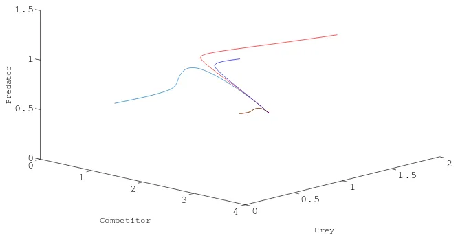
5.1. Numerical example for trnascritical bifurcation
Chooser1=12,b1=10,α =2,a1=2,m=0.5,r2=6,β =5,a2=2,b2=1,r3=1,k=1.5 then system (1.1) admits a transcritical bifurcation at E1(1.2,0,0) with respect to β.(see Fig.
1.)
0
0.5 1
1.5 2 0
1
2
3
4 0
0.5 1 1.5
Prey Competitor
Predator
Fig. 1. Transcritical bifurcation nearE1
Hopf-bifurcation) atE12 as the Jacobian matrixJ(E12)has no zero eigenvalues due to the exis-tence ofE12.
Theorem 1.4. System (1.1) admits a transcritical bifurcation but no saddle-node bifurcation around the equilibrium pointE13 whenr2crosses the critical valuer∗2=βbx.
Proof.Proof is similar to the proof of Theorem 1.3.
Remark 2: System (1) does not undergoes any Hopf-bifurcation around the interior equilib-rium pointE∗as in equation (4),A1>0 andA1A2−A3cannot be equal to zero.
Theorem 1.5. Suppose that 4b1b2a2
k+x∗−m > (
(α+β)2a2
k+x∗−m +b2
(x∗−m)a1
x∗ + r23 k+x∗−m
!)
andr2 >βx∗.
Then the interior equilibrium pointE∗is globally asymptotically stable.
Proof. First note that, E13 is unstable as r2>βx∗ and other boundary equilibrium points are
always unstable whenever they exist.
Consider the following positive definite function aboutE∗
V(t) = (x−x∗−x∗ln x
x∗) + (y−y
∗−y∗ln y
y∗) + (z−z
∗−z∗ln z
z∗)
DifferentiatingV with respect tot along the solution of system (1.1), we get
dV
dt = (x−x
∗){r
1−b1x−αy−a1(xx−m)}+ (y−y∗){r2−b2y−βx}+ (z−z∗){r3−k+ax2−zm}
= (x−x∗){−b1(x−x∗)−α(y−y∗) +a1(x
∗−m)
x∗ −
a1(x−m)
x }+ (y−y
∗){−b
2(y−y∗)−β(x−x∗)}+
(z−z∗){ a2z∗
K+x∗−m− a2z
k+x−m}
≤ −b1(x−x∗)2+ (α+β)|(x−x∗)||(y−y∗)| −b2(y−y∗)2−a2(z−z
∗)2
k+x∗−m +{
(x∗−m)a1
x∗ + r3
k+x∗−m}|x−
We note that ˙V is negative definite if
b1b2a2
k+x∗−m >
1 4
(α+β)2a2
k+x∗−m +b2 (
(x∗−m)a1
x∗ + r32
k+x∗−m )
Thus the condition of Theorem 1.5 implies thatV is a Lyapunov function and hence the theorem follows.
6. Persistence
Biologically persistence means the long time survival of all population in a future time what-ever may be the initial populations. By differential inequality argument we state some result guaranteeing the persistence of all the populations of system (1.1).
Theorem 1.6. (i) If x(t)>m then limt→∞supx(t)≤
r1
b1 (ii) If x(t)≤m and r1b2 >αr2 then
limt→∞infx(t)≥
r1b2−αr2
b1b2
Proof.(i) Whenx(t)>m, dxdt ≤(r1−b1x)x =⇒ limt→∞supx(t)≤
r1
b1
(ii) Whenx(t)≤m, dxdt ≥(r1−b1x)x−αxbr2
2 = (r1− αr2
b2 −b1x)x =⇒ limt→∞infx(t)≥
r1b2−αr2
b1b2
Theorem 1.7. (i) If x(t) >m and r2 > βbr11 then limt→∞infy(t)≥
b1r2−βr1
b1b2 (ii) If x(t)≤m
andr2>βmthen limt→∞infy(t)≥
r2−βm
b2
Proof. when x(t)> m, limt→∞supx(t)≤
r1
b1 then from the second equation of (1) we have
dy
dt ≥(r2−
βr1
b1 −b2y)y =⇒ limt→∞infy(t)≥
b1r2−βr1
b1b2 .
(ii) Ifx(t)≤m, then dydt ≥(r2−βm−b2y)y.
As,r2>βm, this implies that limt→∞infy(t)≥
Theorem 1.8.Ifk>mthen limt→∞infz(t)≥
r3(k−m)
a2 .
Proof.Sincek>mthenk+x−m>k−mand hence− 1
k+x−m>−
1
k−m.
From third equation of (1.1), we have dtdz≥z(r3−ka−2zm) =⇒ limt→∞infz(t)≥
r3(k−m)
a2 .
7. Influence of prey refuge
In the following we shall discuss the influence of prey refuge on each population when the coexistence equilibrium pointE∗ is exists and is stable. It is easy to see that x∗,y∗,z∗ are all continuous differential functions of parameterm.
Now letα be any positive root of equation (4.2).
Thenα = −B± √
B2−4AC
2A where
A=b1a2b2−α βa2+r3b2a1,B=−{r1a2b2−αr2a2−r3b2a1(k−2m)},C=−r3b2a1m(k−m).
Now dα
dm =− dB dm+
1 2
2BdmdB−4AdmdC
√
B2−4AC >0 provided,
a2
a1 > r3
b1 and min
α βa2
a1r3 , r2a2
r1a1
<b2<
α β
b1 . (7.1)
Again dydm∗ =−β
b2
dx∗
dm <0 and dz∗ dm =
r3
a2(
dx∗ dm −1).
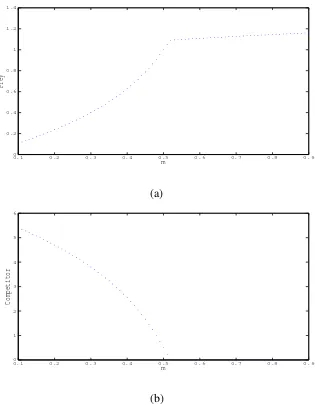
Clearlyx∗is strictly increasing function of parametermwhenever (7.1) holds and increasing the amount of prey refuge leads to the increasing density of the prey species. y∗is strictly decreas-ing function of parametermand increasing the amount of prey refuge leads to the decreasing density of the competitor prey species. The presence of negative term in the third equation in-dicates that increasing the amount of prey refuge may decrease the predator density as long as
7.1 Numerical example for influence of prey refuge
Here we choose a set of parameters r1=12,b1 =10,α =2,a1=2,m=0.5,r2=6,β = 5.5,a2=2,b2=1,r3=1,k=1.5 and in this case interior equilibrium pointE∗is locally asymp-totically stable. Influence of prey refuge on susceptible and infected prey population is given in Fig. 2. and Fig. 3.
0.10 0.2 0.3 0.4 0.5 0.6 0.7 0.8 0.9
0.2 0.4 0.6 0.8 1 1.2 1.4
m
Prey
(a)
0.10 0.2 0.3 0.4 0.5 0.6 0.7 0.8 0.9
1 2 3 4 5 6
m
Competitor
(b)
0.1 0.2 0.3 0.4 0.5 0.6 0.7 0.8 0.9 0.75
0.8 0.85 0.9 0.95 1 1.05 1.1
m
Predator
Fig. 3. Influence of prey refuge on predator population
8. Numerical Simulation
Dynamical behaviour of Leslie-Gower predator-prey model is not affected by refuge. If interspecific competition is allowed into the system, oscillation can emerge. Keeping this in mind, we have taken the rate of interspecific competition low and high. We selectr1=12,b1=
10,α =2,a1=2,m=0.5,r2=6,β =5.5,a2=2,b2=1,r3=1,k=1.5. Our numerical result shows that system (1) converges to this pointE∗(1,0.5,1)(see Fig. 4.).
0.8 1
1.2 1.4 1.6
1.8 2
0 0.5 1 1.5 2 0.8 1 1.2 1.4 1.6 1.8 2
Prey Competitor
Predator
Further we consideredr1=4,b1=1,α =1.2,a1=2,m=0.5,r2=6,β =5,a2=1.5,b2= 1,r3=2,k=0.25, the system oscillates near this equilibrium point E∗(57,177,1321). Also some chaotic type oscillation is observed (see Fig. 5.).
1.576 1.577
1.578 1.579
1.58
1.581
0 0.5 1 1.5 2 2.5 3
x 10−7 1.768 1.769 1.77 1.771 1.772 1.773 1.774 1.775 1.776 1.777 1.778
Prey Competitor
Predator
Fig. 5. The system (1.1) is unstable and chaotic type oscillation observed
In the first case α β = 11 and b1b2= 10 that indicates interspecific competition is low. In the second case α β =6 andb1b2=1 that implies interspecific competition is high i.e all the equilibrium points are unstable in nature. That causes chaotic type motion.
9. Discussion
Thus our system is either stable or unstable around the coexistence equilibrium point. We have found five possible equilibria, namely trivial equilibrium pointE0, axial equilibrium pointE1, predator free equilibrium point E12, competition free equilibrium point E13 and coexistence equilibrium pointE∗. Here the boundary equilibrium pointsE0,E1,E12 are always unstable in nature where asE13 may be stable when the intrinsic growth rate of competitor remains below certain threshold value (r2<βxb). Local stability at the coexistence equilibrium point can be
checked from the condition of Theorem 1.2. We observed that from the numerical simulation that chaotic motion can arrise if the condition of Theorem 1.2 is violated. Further we have de-rived a sufficient condition for global stability condition of the coexistence equilibrium point. By using differential inequality argument we found persistence condition of the population. The novelty of our paper is the occurrence of transcritical bifurcation but no Hopf-bifurcation around the equilibria. Though Mukherjee [14, 16] showed Hopf-bifurcation in his system and did not carried out local bifurcation analysis.
Conflict of Interests
The authors declare that there is no conflict of interests. REFERENCES
[1] G. Birkhoff, C.G. Rota, Ordinary Differential Equation, Ginn and Co., Boston (1982).
[2] R. Cressman, J. Garay, A predator-prey refuge system: Evolutionary stability in ecological systems, Theor.
Popula. Biol. 76 (2009), 248-257.
[3] F.D. Chen, L.I. Chen, X.I. Xie, On a Leslie-Gower predator-prey model incorporating a prey refuge.
Nonlin-ear Anal., Real World Appl. 10 (2009), 2905-2908.
[4] L.S. Chen, F.D. Chen, L.J. Chen, Qualitative analysis of a predator-prey model with Holling type II functional
response incorporating a constant prey refuge. Nonlinear Anal., Real World Appl. 11 (2010), 246-252.
[5] L.S. Chen, F.D. Chen, Global analysis of a harvested predator-prey model incorporating a constant prey
refuge. Int. J. Biomath. 3 (2010), 205-223.
[6] E. Gonz´alez-Olivares, R. Ramos-Jiliberto, Dynamic consequence of prey refuges in a simple model system:
More prey, fewer predators and enhanced stability. Ecol. Mod. 166 (2003), 135-146.
[7] L.L. Ji, C.Q. Wu, Qualitative analysis of a predator-prey model with constant-rate prey harvesting
incorpo-rating a constant prey refuge. Nonlinear Anal., Real World Appl. 11 (2010), 2285-2295.
[9] T.K. Kar, Stability analysis of a prey-predator model incorporating a prey refuge. Commun. Nonlinear Sci.
Numer. Simul. 10 (2005), 681-691.
[10] T.K. Kar, Modelling and analysis of a harvested prey-predator system incorporating a prey refuge. J. Comput.
Appl. Math. 185 (2006),19-33.
[11] P.H. Leslie, J.C. Gower, The properties of a stochastic model for the predator-prey type of interaction between
two species, Biometrika 47 (1960), 219-234.
[12] X. Liu, M.A. Han, Chaos and Hopf bifurcation analysis for a two species predator-prey system with prey
refuge and diffusion. Nonlinear Anal., Real World Appl. 12 (2011), 1047-1061.
[13] R.M. May, J.R. Beddington, C.W. Clark, S.J. Holt, R.M. Laws, Management of multi-species fisheries,
Sci-ence 205 (1979), 267-277.
[14] D. Mukherjee, The effect of refuge and immigration in a predator-prey system in the presence of a competitor
for the prey. Nonlinear Anal., Real World Appl. 31 (2016), 277-287.
[15] D. Mukherjee, The effect of prey refuges on a three species food chain model. Differ. Eqns. Dyn. Sys. 22 (4)
(2014), 413-426.
[16] D. Mukherjee, Study of refuge use on a predator-prey system with a competitor for the prey. Int. J. Biomath.,
(10)2 (2017), Article ID 1750023.
[17] D. Mukherjee, Bifurcation analysis of a Holling type II predator-prey model with refuge. Int. J. Bifurcation
Chaos (2017), in press.
[18] J. Sotomayor, Generic bifurcations of dynamical systems. In : Peixoto, M.M.(eds.) Dyn. Sys., Academic
Press, New York (1973), 549-560. .
[19] Y.D. Tao, X. Wang, X.Y. Song, Effect of prey refuge on a harvested predator-prey model with generalised
functional response. Commun. Nonlinear Sci. Numer. Simul. 16 (2011), 1052-1059.
[20] P. Turchin, I. Hanski, An empirically based model for latitudinal gradient in vole population dynamics, Am
Nat.149 (1997), 842-874.
[21] F.J.F. van Veen, P.D. van Holland, H.C.J. Godfrey, Stable coexistence in experimental insect communities
due to density and trait mediated indirect effects, Ecology 12 (2005), 241-245.
[22] Q. Yue, Dynamics of a modified Leslie-Gower predator-prey model with Holling-type II schemes and prey