Geographics
Methodology
A semiparametric cluster detection method
—
a comprehensive
power comparison with Kulldorff
’
s method
Shihua Wen*
1and Benjamin Kedem
2Addresses:1Abbott Laboratories, Abbott Park, IL, USA and2Department of Mathematics, University of Maryland, College Park, USA
E-mail: Shihua Wen* - [email protected]; Benjamin Kedem - [email protected] *Corresponding author
Published: 31 December 2009 Received: 12 September 2009
International Journal of Health Geographics2009,8:73 doi: 10.1186/1476-072X-8-73Accepted: 31 December 2009 This article is available from: http://www.ij-healthgeographics.com/content/8/1/73
©2009 Wen and Kedem; licensee BioMed Central Ltd.
This is an Open Access article distributed under the terms of the Creative Commons Attribution License (http://creativecommons.org/licenses/by/2.0), which permits unrestricted use, distribution, and reproduction in any medium, provided the original work is properly cited.
Abstract
Background: A semiparametric density ratio method which borrows strength from two or more samples can be applied to moving window of variable size in cluster detection. The method requires neither the prior knowledge of the underlying distribution nor the number of cases before scanning. In this paper, the semiparametric cluster detection procedure is combined with Storey’s q-value, a type of controlling false discovery rate (FDR) method, to take into account the multiple testing problem induced by the overlapping scanning windows.
Results: It is shown by simulations that for binary data, using Kulldorff’s Northeastern benchmark data, the semiparametric method and Kulldorff’s method performs similarly well. When the data are not binary, the semiparametric methodology still works in many cases, but Kulldorff’s method requires the choices of a correct probability model, namely the correct scan statistic, in order to achieve comparable power as the semiparametric method achieves. Kulldorff’s method with an inappropriate probability model may lose power.
Conclusions: The semiparametric method proposed in the paper can achieve good power when detecting localized cluster. The method does not require a specific distributional assumption other than the tilt function. In addition, it is possible to adapt other scan schemes (e.g., elliptic spatial scan, flexible shape scan) to search for clusters as well.
Background
Scan statistics arise when scanning in time, or space, or both, looking for clusters of certain events or cases. Here theclustercan be defined as a certain spatial or temporal subregion where the the probability distribution of an event is different from that in the rest of the region. More generally, a cluster is a subregion where the behavior of an observable is different from the behavior of the observable in the rest of the region. For instance, a subregion comprised of several counties with higher rate of one certain type of cancer than the rate of other counties in the study region defines a cancer cluster [1].
Besides epidemiology, more examples of clusters can be found in many other fields, including criminology, genetics, mining, astronomy, and so on. See Glaz and Balakrishnan (1999), Glaz et al. (2001) [2,3].
As a contemporary research topic, research on scan statistics can be traced back to the 1960’s [4]. Since then it came out many scan statistics methods, such as scan statistics with Poisson assumptions [3], scan statistics in purely temporal domain [5], Upper-level set scan [6-8], Flexible shaped scan [9,10], etc. Among them, Kulldorff’s spatial scan statistics has been one of the most popular
BioMedCentral
methods and has been applied in many scientific fields for detecting either purely spatial or higher dimensions clusters, e.g. space-time scan [11-15]. However, Kull-dorff’s method requires assumptions on the underlying distribution (Bernoulli, Poisson, exponential, etc.) of the scan region. If an inappropriate model is chosen, the power of cluster detection may significantly decrease [16]. In addition, the method requires knowledge of the number of events over the region of interest for Monte Carlo hypothesis testing.
Kedem and Wen (2007) [16] proposed a semiparametric cluster detection procedure which requires much less than complete distributional assumptions, and which does not require the number of cases prior to scanning. They also performed a limited power study showing that when data are largely compatible with the Bernoulli or Poisson assumptions, the semiparametric method could be as powerful as the focused test [17] and as Kulldorff’s method, but the semiparametric method could achieve higher power when data deviate from the Bernoulli or Poisson assumptions. However, the power study did not involve a scanning stage where the moving window scan the whole study region for cluster candidates. It was assumed that the cluster was already known, and only wanted to compare which method, either Kulldorff’s method or the semiparametric one, had higher power in detecting the difference correctly between the cluster region and the background. Hence, the power study was called limited. Although the case study for the North Humberside childhood leukemia data set [11,18] of the paper had the scan stage, the significant level was not adjusted for multiple testing yet.
In this paper, we extended the original semiparametric cluster detection procedure by incorporating Storey’s q-value method [19,20], a type of false discovery rate (FDR) methodology [21], to take into account the multiple testing problem inherent in cluster detection. A comprehensive power study was then conducted using Kulldorff’s northeastern benchmark data set [22] for binary power comparison and generated quantized normal data for non-binary power comparison. The results show that for binary data the semiparametric method and Kulldorff’s method are quite comparable. However, when data are not binary, the semiparametric method performs well regardless of the probability model whereas Kulldorff’s method requires the correct model in order to get a comparably good power. When the chosen model is inappropriate, Kulldorff’s method may not achieve good power. This findings are also consistent with the limited power study performed in Kedem and Wen (2007) [16]. The extended semipara-metric method was again illustrated by the North Humberside childhood leukemia data set.
Methods
Kulldorff’s Scan Statistics
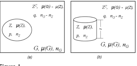
Kulldorff’s scan statistics method uses a large collection of overlapping scan windows to detect clusters, both the location and the size, and evaluate their significance. See Figure 1 for an illustration. For spatial data, the method first imposes a circular window on a map and let the circle centroid move across the study region. For any given centroid, the radius of the window varies continuously from zero to some upper limit. Usually this upper limit is set to be the radius which covers 50% of the whole study region or population. In this way, the method generates a large set of scan windows ℤ with different centroid and size. Under the null hypothesis of no cluster, the underlying behavior of the data through-out the whole study region is the same. Under the alternative hypothesis, there is at least one scan window for which the underlying behavior inside the window is different as compared with its complement, which means any scan windowZ(Z∈ℤ) could be a potential cluster. In practice, some data are updated periodically. In such cases, space-time scans are used [13,23]. The scanning procedure of space-time scans is almost identical to the purely spatial scan, except that the scan window becomes a three-dimensional cylinder (see part (b) of Figure 1) instead of two-dimensional circle. Since the statistical formulation of space-time scan is identical to the two-dimensional case, we only describe the 2D purely spatial scan in this paper.
By Kulldorff’s scan statistics method, each scan window Zis associated with a likelihood ratio test statisticl(Z) which can be computed based on the chosen underlying probability model and the observed data. The scan window associated with the maximuml (Z) is defined as the primary cluster candidate occurring not by random chance. The maximum likelihood ratio itself is called the Kulldorff’s spatial scan statistic, and the null hypothesis is rejected for large value. After the spatial
Figure 1
scan statistic and the primary cluster candidate are determined, a Monte Carlo hypothesis procedure or a permutation test procedure is executed to generate the probability distribution of Kulldorff’s scan statistic under the null hypothesis of no cluster in the study region, and ap-value is obtained [23,24].
For different types of data, Kulldorff proposed different scan statistics based on the corresponding probability models.
Bernoulli model
Bernoulli-based scan statistic is used when individual entities have only two states such as an individual person having cancer or not. The part (a) of Figure 1 shows a typical setup of Kulldorff’s scan statistics method. The following notation is used.
•G: the whole study region
•Z: the scan window
• μ(G): the total number of individual entities (e.g. people) inG
•μ(Z): the number of individual entities inZ
•nG: the total number of events inG
•nZ: the number of events insideZ
• p: the rate of events that occurred inside the scan windowZ
•q: the rate of events that occurred outside the scan windowZ
We test the null hypothesisH0:p=qof no cluster. It can
be shown that, for an alternative hypothesis that there is a hot spot cluster p>q, each scan windowZ invokes a likelihood ratio test statistic as in equation (1):
( )
( ) ( ) ( )( ( ) ( )) ( )
Z
pnZ p Z nZ qnG nZ q G Z nG nZ p
1 1
0
n
nG( p ) ( )G nG p q
,
,
1 0
1
if
otherwise
(1)
Where pˆ0 nG( )G , ˆp nZ( )Z , ˆq( ( )(nG nZG ( ))Z) . If we were scanning for cold spots, then“>”would change to“<”; if for either hot or cold spots, then it would be “≠” (Kulldorff, 1999). After all the l (Z) are computed, we determine the primary cluster candidate Zˆ from
max ( ) ( )
Z Z Z
, and reject the null for large values of
( )Z . A Monte Carlo based p-value can be obtained from randomization of the cases across the whole study region given the total number of cases.
Poisson model
Poisson-based scan statistic is used for the comparison of the number of cases inside and outside a scan window
when searching for clusters. Suppose we have a study region composed of I sub-regions. For i = 1, 2,..., I, assume the number of events xi which occur in an
“interval”μ(Ai) is a Poisson process with intensity ratep inside the scan window and q outside, respectively. Similarly to the Bernoulli model, the likelihood ratio test statistic for each scan windowZ for testingH0: p=q is
shown in equation (2):
( ) ,
,
( )
Z nZe Z nG nZnG eZ n e
n n n
Z Z
Z G Z
if
otherw
1 iise
(2)
where nZ is the observed number of cases inside the scan windowZ, andeZis the expected number of cases inside the scan window Zunder the null hypothesis of no cluster. As before, if we were scanning for a cluster other than hot spot, we simply change the inequality sign as needed. After getting all the l (Z)’s, find ( )Z and the Monte Carlo based p-value. When p is small, e.g. a rare disease, the Poisson model gives a close approximation to the Bernoulli model and obtains very similar results [11].
Ordinal model
Jung et al. (2006) [15] proposed an ordinal model, which is used when individual entities have K > 2 ordinal categories such as the different stages of a kidney disease, stage 1, 2, 3, 4 and 5. A higher category may reflect a more serious cancer stage. Suppose the study region consists of I sub-regions and the variable of interest is recorded in K categories. Each individual in the analytical sample falls into one category. Let cik be the number of individuals in locationiwho fall into category k, where i = 1, 2,..., I and k = 1, 2,..., K. Let Ck =Σicikbe the number of observations in category k across the study region, and C= ΣkCk = ΣkΣi cik be the total number of observations in the whole study region.
The null hypothesis of no cluster in this model means p1 = q1, ..., pk = qk, where pk and qk are the unknown probabilities that an observation belongs to category k inside and outside the scanning window, respectively. To detect subregions with high rates of higher stages as compared with the rest of the area, one possible a l t e r n at i v e hyp o t he s i s co u l d be pq qp pK
q K 1
1 2 2
.
( )
( )
( / )
,
, ,
Z
pkcik i Z
qkcik i Z k
Ck C Ck k
pk qk
otherwise
1 kk K
1 2, ,,
(3)
where pˆk and qˆk are the MLEs ofpk and qk under the alternative hypothesis. A“Pool-Adjacent-Violators” algo-rithm [25,26] can be applied to compute pˆk and qˆk. After all thel(Z)’s are obtained, get ( ),Z Z. A Monte Carlo based p-value can be obtained by randomization of the observations across the study region given the total number of observations in each category,C1,C2,...,
CK.
The above gives a brief summary of Kulldorff’s scan statistics under Bernoulli model, Poisson model, and ordinal model, respectively. As for other types of scan statistics in Kulldorff’s scan statistics family, see Huang et al. (2007) for the exponential model [14], Kulldorff et al. (2007) for the multivariate scan model [27], Kulldorff et al. (2009) for the normal model [28], and Kulldorff et al. (2006) for elliptic window scans [29].
Kulldorff’s method has been applied successfully in many applications. However, it requires assumptions on the underlying distribution (Bernoulli, Poisson, expo-nential, etc.) of the scan region and the knowledge of the number of events over the region of interest for Monte Carlo hypothesis testing. Moreover, It may take con-siderable amount of computation time to obtain the Monte Carlo basedp-value.
Semiparametric Scan Statistics Method
Kedem and Wen (2007) [16] proposed a semiparametric scan statistics method for cluster detection using a density ratio model studied by Fokianos et al. (2001) and Qin and Zhang (1997) [30,31]. Similar to Kull-dorff’s scanning procedure, the semiparametric scan statistics method also uses a movable variable-size window to scan the whole study region, but performs for each window a two-sample test. Because the moving window generates a large set of overlapping scan windows, it results in a large number of semiparametric test statistics and their corresponding p-values as well. The largest test statistic is defined as the semiparametric scan statistic. To take account of the multiple-testing problem induced by the multiple scanning windows, the originalp-values are replaced by Storey’sq-values, a type of controlling false discovery rate (FDR) methodology. Then the primary cluster candidate will be the window (subregion) corresponding to the largest test statistic or
equivalently the smallest q-value. If this q-value is less than a pre-decided level (say 0.05), we claim the located cluster candidate is a true cluster. We describe briefly the semiparametric scan statistics method and the q-value FDR methodology in the following subsections.
Semiparametric Test Statistics
Using Kulldorff’s circular window scan scheme, consider a scan window which separates the study region into two parts. This results in two samples,
x
x
1 11 12 1 1
2 21 22 2 2
1
2
( , , , ) ~ ( )
( , , , ) ~ ( )
x x x g x
x x x g x
n
n
wherex1is the sample inside the scanning window with
sample size n1, and the x2 is the sample outside the
scanning window with sample size n2, gj(x) is the
probability density function of xji, j= 1, 2, i = 1,..., nj. Choosing the sample outside the scanning window as the reference sample andg2(x) as the reference density, it
is assumed that the density ratio between the density inside the scanning window and the reference density has an exponential form
g x
g x x
1
2 1 1
( )
( )exp{ h( )}.
Here h(x) is a known vector-valued function of xwhich may take on a scalar form such as x or a vector-valued form such as (x,x2)’,a1is a scalar, butb1can be a scalar
or vector depending onh(x). Clearly,b1=0impliesa1=
0. Therefore, b1 = 0 implies the null hypothesis of no
cluster is accepted since the probability distribution inside and outside the scanning window are equal. See Kedem and Wen (2007)and Fokianos et al. (2001) [16,30] for the general setup form ≥2 samples.
Following the profiling procedure discussed in Qin and Lawless (1994) [32], Qin and Zhang (1997), and Fokianos et al. (2001), we obtain the log-likelihood:
(1, 1) log[ 1 exp{1 1 ( )}] [ ( )]
1
1 1 1
1
hti hxi n
j j 11
1
n
(4)
wheretiisith observation in thecombinedsamplet= (x1,
x2)’, andr1=n1/n2.
n ˆ
ˆ ( , )
1 1
1 1
N0 (5)
where Σ is a special case of S-1V S-1 under q = 1. See Appendix 2 for the definition of the matricesS andV.
The maximum likelihood estimator of the reference (background) distribution function from the combined sample is given as,
ˆ( ) ( )/
exp{ ˆ ˆ ( )}
G x I ti x n
ti
i n
21 1 1 1
1 h
(6)
Kedem and Wen (2007) [16] proposed three test statistics for testing the null hypothesis H0: b1 = 0,
which means no cluster.
c1test statistic
1 1 1 1
1 1 2
nˆ Var t
( )
[ ( )] ˆ
h (7)
wherer1=n1/n2andVar[h(t)] is the covariance matrix
of h(t) with respect to the reference distribution. It follows underH0thatc1is approximately distributed as
Chi-square with v degrees of freedom, where v is the dimension ofb1, which is the same as the dimension of
the function h(x). The null hypothesis H0: b1 = 0 is
rejected for large values of c1. In practice, Var [h(t)] is
replaced by its estimator [16,30]. In addition, if the data are binary (0-1), the c1 statistic can be simplified to a
close form of equation (15) in the Appendix 1.
c2test statistic
2 1
n(H c) (H H ) (H c) (8)
tests for a general linear hypothesis Hθ = c, where θ =
(1,,w,1,,w ) ,wis the total number of samples excluding the reference sample. H is p’ × [(1 + v)w)] predetermined matrix of rank v’, v’ < (1 + v)w, c is a vector in v, and the variance-covariance matrix Σ =
S-1V S-1. It follows under H
0 that c2 is asymptotically
distributed as c2with (v’) degrees of freedom provided
the inverse exists [33], andH0is rejected for large values.
This test is useful when one wants to borrow informa-tion from other sources besides the current study region, although we did not use it in this paper.
Likelihood ratio test statistic
LR
ti i
2 0
2 1
1 1
1 1 1
1
[ ( , ) ( , )]
log[ exp{ ( )}]
0
h
n n
j j
n
x
n
2
2 1
1 1 1 1
1
1
[ ( )]
log( )
h
(9)
Under H0: b1 = 0, LR is asymptotically approximately
distributed as Chi-square withvdegrees of freedom, and H0is rejected for large values. Recallvis the dimension
ofb1and it depends on the choice of the functionh(x).
Similarly, when the data are 0-1 binary, the likelihood ratio statistic reduces to equation (16) in the Appendix 1.
Storey’s FDR Method and q-value
Controlling the false discovery rate (FDR) is a less conservative way to handle multiple testing problems. It was first proposed by Benjamini and Hochberg (1995) [21]. Since then, the FDR methodology has been further developed and applied to many fields, especially in genomic research [34-36]. FDR is defined to be the expected proportion of falsely rejected hypotheses (false positives) as in equation (10),
FDR E V
max R E
V
R R Pr R
( , )1 | 0 ( 0) (10)
whereVandRare defined in Table 1. From the table it is clear that ifm=m0, which means all the null hypotheses
are true, then FDR is equivalent to the family-wise error rate (FWER). To see that, recalling FWER is defined as P (V≥1),m=m0makesS= 0, and hence EVR|R0 = 1
for allR> 0, and thereforeFDR= 1 *P(R> 0) =P(V≥1) = FWER. If m0 <m, then FDR ≤ FWER, which means a
potential gain in power at the cost of increasing the likelihood of making type I errors [21].
Storey (2002) and Storey et al. (2004) [19,37] improved the original Benjamini and Hochberg’s FDR methodol-ogy by estimating theπ0=m0/m, the proportion of true
null hypotheses. In addition, Storey used positive FDR (pFDR) as in equation (11) instead of FDR as in equation (10).
pFDR E V
R R
| 0 (11)
In many cases, whenm, the total number of hypotheses, is large, it easily to have significant ones, which makesPr (R> 0)≈1. Thus, pFDR (eq. 11) is close to FDR (eq. 10) in numerical value, but pFDR has some conceptual advantages. A thorough motivation of using pFDR rather than FDR can be found in Storey (2003) [20].
Table 1: Classification ofmhypotheses tests
Hypothesis # of Accept # of Reject Total
# of true nulls U V m0
# of true alternatives T S m1
The q-value is defined to be the pFDR analogue of the p-value. It gives the error measurement with respect to pFDR for each observed test statistic of each particular hypothesis. More precisely, theq-value of one particular observed test statistic T = t from a set of tests can be defined to be
q t pFDR
t
-value( ) inf ( ),
:
(12)
where Γa is a nested significance region at levela[19]. This means the q-value is the minimum pFDR at which the corresponding test may be called significant. In this way, q-value simultaneously takes into account the multiple testing problem.
In our semiparametric scan situation, we generate a lot of overlapping scan windows, and each window associates to a hypothesis test and a test statistic, so m here is usually large. Because of the large m, we adopted the algorithm in Storey et al. (2003) [35] to estimated the q-value for each scan window as follows:
1. Obtain thep-value for each scan window, and sort
p( )1 p( )2 p( )m.
2. Estimateπ0 using a cubic spline function. First, for a
range ofl, say l= 0, 0.01,...,0.95, calculate
ˆ ( ) #{ ( ) }
( ) .
0
1
p j
m for each
Then let fˆ( ) be the natural cubic spline of ˆ ( )0 . Finally, set the estimate of π0to be ˆ0 fˆ( )1 .
3. Calculate
ˆ( ) min ˆ
#{ ( ) } ˆ ,
( ) ( )
( )
q p mt
p j t p
m
t pm m
0
0 0 where tt1.
4. Fori=m -1,m -2,...,1, calculate the estimatedq-value for the ith most significant one as
ˆ( ) min ˆ
#{ ( ) )} min
ˆ ( ) , ˆ( ( )
( )
q p mt
p j t
mp i
i q
i t pi
0 0
pp(i)) .
1
5. Choose the region with the largest test statistic, for example, the largest likelihood ratio test statistic, as the primary cluster candidate, and itsq-value is q(p(1)), the smallest q-value among all the tests. If q(p(1)) is less than a pre-decided false discovery rate, say q(p(1)) < 0.05, we claim there is clustering and the located primary candidate is a true cluster region.
The semiparametric approach has several advantages. First, the reference (or background) distribution, G(x), and all the parameters such asb1are estimated from the
combined data t, not just from a single sample either inside the window or outside the window. Second, for a properly chosenh(x), the above tests are quite powerful. The simulation results indicate that thec1-test competes
well with the corresponding F-test [30]. Moreover, Gagnon (2005) [38] shows that for m = 2 the c1-test
can be more powerful than the common t-test for a known h(x) but unspecified distributions. Third, in testing equidistribution, other than an assumption regarding the tilt function h(t), the semiparametric density ratio method does not require distributional assumptions. Fourth, the semiparametric method can be applied to either continuous or discrete distributions. Fifth, since the asymptotic distributions of the above mentioned test statistics are known, in principle there is no need for the time consuming Monte-Carlo methods to compute thep-values. Lastly, Storey’sq-value method can adjust the original p-values, and easily handles the multiple testing problem inherent in cluster detection.
Data Sets for the Power Comparison
Both Kulldorff’s and the semiparametric scan statistics methods are suitable for both binary and non-binary data. So we use both types of data to perform the simulated power study. The following two subsections give a brief description of the binary and the non-binary data sets used in the study.
Binary Data Set—Northeastern USA Benchmark Data
For binary data scans, we use Kulldorff’s Northeastern USA purely spatial benchmark data [22] which consist of 245 counties in northeastern United States, from Maine, New York, Rhode Island, Pennsylvania, Maryland, Washington DC, among others. Each county is graphi-cally represented by its centroid coordinates. The case data, which is the number of people who have breast cancer, are aggregated to each county centroid with the total number of cases in northeastern states (the whole study region) being fixed. The population data of each county are based on the female population of the 1990 census. The benchmark data set contains two types of data, hot-spot clusters and global clustering data, generated in different ways.
Hot-spot clusters
risk of breast cancer is much higher than in the rest of area. Three types of clusters, rural, urban, and mixed, are generated depending on the location of the cluster. A rural cluster is the type of cluster where a small population relative to a large graphical area, such as the Grand Isle county in north Vermont close to the Canadian border. An urban cluster is the type of cluster which has a large population relative to a small graphical area, such as New York county which includes Manhat-tan. A mixed cluster is the type of cluster where a big city is surrounded by rural areas, such as Allegheny county in western Pennsylvania where Pittsburgh is. See Kulldorff et al. (2003) [22] for more detail.
Global clustering
Data are generated by purely second-order clustering model, where any one particular case is randomly located, but the location of cases are dependent on each other. Thus, under the alternative hypothesis of global clustering, cases are clustered wherever they occur in the region. In this benchmark data set, a certain number of cases are first generated to be randomly located throughout the whole northeastern states. These original cases then generate other new cases close by. If each original case generates one additional case, we call them twins; if two additional cases are generated, we call them triplets. The case generation is based on a global chain rN-nearest neighbor rule. The global chain is constructed by a Hamiltonian cycle chain which passes through as many counties as possible exactly once and any two counties next to each other on the chain always border each other graphically. For twins, the additional case is assigned to countyjifΣkI(dik<dij)nk<rN≤ΣkI(dik≤ dij)nk, wherenk is the population size of county k, N =
Σknkis the total population size,ris some constant in the interval of (0,0.5) with the bigger r the broader geographical area to spread the cases, and dij is the distance in one particular direction along the chain connecting county i and county j. For triplets, the two new cases are assigned in opposite directions along the chain. Data sets corresponding to different r were generated from a probability distribution or be deter-mined in advance. Notice that although the data generation mechanism of the second-order clustering model is very different with the first-order clustering model, the resulting point patterns may look quite similar, and hence indistinguishable.
Both hot-spot and global clustering data sets in this benchmark data set have two separate groups of data with a total of 600 and 6000 simulated cases, respec-tively. For each group the same null hypothesis of no cluster is used where the relative risk for each county is
equal, and the cases as well as their locations are independent of each other. In order to perform power comparison, 100000 random data sets with a total of 600 and 6000 cases were generated under the null hypothesis, respectively. They are used to estimate the critical cut-off point of significance for each group. For the alternative hypothesis of clusters which are called scenarios in this paper, 10000 random data sets per scenarios were generated to estimate the power using the previous determined cut-off points.
For each group of fixed total cases (600 or 6000 cases), Kulldorff generated 35 hot-spot clustering scenarios and 26 global clustering scenarios for his power comparison. For instance, a scenario of“rural and urban 600, size 4” means that the total of number of cases in the whole study region is 600 and the study region contains two hot-spot clusters. One cluster is in a rural region including four counties, and the other one is in an urban region including four counties also. A scenario of
“global clustering twin 6000, exponential 0.02” means that the total number of cases is 6000 and the cases are generated under the alternative hypothesis of global clustering. The value r is not constant but randomly generated from an exponential distribution with mean 0.02 among the data set generated under this scenario.
We did not use all the scenarios in Kulldorff’s North-eastern US benchmark data in this paper. Instead, we randomly chose one or two scenarios from each clustering pattern. Finally, nine hot-spot clustering scenarios and six global clustering scenarios were used in our power study for the binary data case. After selecting these scenarios, Kulldorff’s method with the Poisson model (Bernoulli model is also appropriate) and the semiparametric method with the tilt functionh (x) = x were applied to the same data sets in each scenario to compare the power. Because data are binary, the simplified semiparametric likelihood ratio test statistic (eq. 16) is used in the computation. All the tests are two-sided to detect for either high or low valued clusters.
Non-binary Data Set—Ordinal Categorical Data
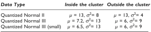
The ordinal categorical data are generated from quantized normal data which truncate the integer part of the original data generated from normal distribution. We refer to quantized normal II and quantized normal III data as in Kedem and Wen (2007) [16]. The quantized normal II data are derived from normal data with the same mean but relatively large variance difference inside and outside the cluster region (inside variance is twice of the outside variance). The quantized normal III data are derived from normal data with both different mean and variance inside and outside the cluster region. To see how Kulldorff’s and the semiparametric methods perform when the difference (in mean) between the cluster and the non-cluster region is small, namely a more difficult cluster to be detected, the data set“Quantized Normal III (small)”was generated. We did not generate data under quantized normal I (same variance, different mean) mechanism, because it has shown that as long as the mean difference is reasonably large, Kulldorff’s method with even an inappropriate scan statistic still would work [16]. Table 2 lists the mean and variance parameters used in this paper to generate the quantized normal data
For each type of data, the average sample size within each state is around 130, hence a total number of
130 * 18 = 2340 observations in each generated data set. Cluster patterns included single cluster and multiple clusters for Quantized Normal II, Quantized Normal III, and Quantized Normal III (small) data, respectively. To perform the power comparison within a reasonable time scale, we used 100 runs, namely 100 random data sets, per cluster pattern in our power comparison study. The single clusters means only one state was randomly chosen as the cluster region. By multiple clusters we mean four states were randomly chosen simultaneously as the cluster region, where the four states are not necessarily contiguous. Notice that multiple clusters constitute a stronger clustering pattern which in general is easier to detect.
In our power comparison for non-binary ordinal categorical data, Kulldorff’s method chose Poisson model (inappropriate model) and the ordinal model (correct model) using SaTScan v7.0.1 http://www.sats-can.org/. 999 replications were used to decide thep-value under each model. The semiparametric method chose the vector tilt functionh(x) = (x,x2)’. Observe that it is also appropriate to chooseh(x) = (x,x2)’for binary data case, because in that case the coefficient ofx2term is 0. See Appendix 1 for detail.
Results
Power Comparison
We compared the power of Kulldorff’s and the semi-parametric scan statistics methods in detecting potential clusters. Because there are various cluster patterns, either single or multiple clusters, and each cluster region may contain one or more counties or states, for simplicity, in our power comparison we more focus on detecting the existence rather than the precise delineation of the cluster region. For instance, for a data set with a pattern of multiple cluster regions and multiple counties in each cluster region, we deem the detection successful when-ever a significance (i.e.,p-value orq-value less than 0.05) is obtained. We do not strictly require the detected cluster region to be exactly the same as originally simulated. The detected cluster region could fully or partially cover the desired area.
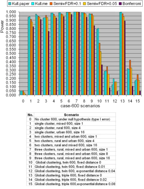
Comparison for Binary Data
The results of power comparison for the binary case-population data using the northeastern US benchmark data set are shown in Figures 3 and 4 for a total number of 600 and 6000 cases, respectively. Kulldorff’s method used Poisson model, and the semiparametric method used the likelihood ratio test. All tests are two-sided tests. The radius of the scan window varies continuously from covering one county to covering no more than 50% of the whole study region. In each figure, scenario 0 is Figure 2
Map of the US middle west and south states used in the simulation for non-binary data.The included states are denoted with color and the abbreviation of their state names. The state Illinois with red color is illustrated as one possible cluster region in our simulated data.
Table 2: Parameters for Generating the Ordinal Categorical Data from Quantized Normal
Data Type Inside the cluster Outside the cluster
Quantized Normal II μ= 13,s2= 8 μ= 13,s2= 4
Quantized Normal III μ= 7.2,s2= 13 μ= 6,s2= 9
under the null hypothesis of no cluster, scenarios 1 to 9 are hot-spot clustering scenarios, and scenarios 10 to 15 are global clustering scenarios. Each scenario contains five quantities. They are “Kull.paper”, “Kull.me”,
“SemiwFDR = 0.1”, “SemiwFDR = 0.05”, and “ Bonfer-roni”. “Kull.paper” is the corresponding power copied from Kulldorff et al. (2003) paper [22].“Kull.me”is the corresponding power computed by us based on Kull-dorff Poisson model. It is shown from Figure 3 and 4 that the column of “Kull.paper” is almost equal to the column of“Kull.me”, which confirms the validity of our computation. So in the latter section, we will use
“Kulldorff’s method” without distinguishing these two power results. “SemiwFDR = 0.1” is the corresponding power computed based on semiparametric method with a q-value significance level 0.1. “SemiwFDR = 0.0.5” is the corresponding power based on semiparametric method with a q-value significance level 0.05. The smaller the q-value significance level is, the harder it is to reject the null hypothesis, hence the lower the power to detect the cluster. “Bonferroni” is the corresponding
power computed based on semiparametric method using Bonferroni correction with 5% family-wise error rate, where the original obtained p-values are multiplied by the number of tests to obtain Bonferroni corrected p -values. If at least one Bonferroni correctedp-value is less than 0.05, we claim there is clustering. As we know Bonferroni correction is a popular but conservative approach to handle multiple testing problems, we expect column of “Bonferroni” should have the lowest power among the five.
For scenario 0, both Figures 3 and 4 show that the type I error of Kulldorff’s method are all exactly 0.05 for both 600 cases and 6000 cases. This is expected since Kulldorff’s method uses a Monte Carlo procedure to derive the cut-off point for the corresponding signifi-cance level. The power from the semiparametric method under theq-value significance level of 0.1 is 0.052 for the 600 cases, and 0.054 for the 6000 cases, almost equal to Kulldorff’s type I error level. Notice that higherq-value significance level means in favor of the alternative. If the Figure 3
Power comparison for binary type data between Kulldorff’s and the Semiparametric method with the likelihood ratio test using the northeastern US benchmark data with totally 600 simulated cases.
Figure 4
q-value significance level is lower down to 0.05, the type I error of the semiparametric method reduced to 0.027 for both cases. It shows that if one wants to make the power comparison under exactly the same type I error level, say 0.05, theq-value significance level must be set in the interval between 0.05 to 0.1. In addition, the type I error of the semiparametric method with Bonferroni correction is the lowest, which is not a surprise, since Bonferroni correction is most conservative.
For scenarios No. 1 to 9, both figures show that the two methods work very well in detecting hot-spot clusters, but Kulldorff’s method seems to be slightly more powerful. When the study area has a stronger pattern of clustering, such as containing more cluster regions, the power of both methods increases, which demonstrates the validity of the two methods. For instance, scenario No. 6 in Figure 3 has a total of 600 cases and two cluster regions where each cluster region contains 16 counties. The power of Kulldorff’s method is 0.996, whereas the power of semiparametric method with q-value signifi-cance level of 0.1 and 0.05 obtain the power 0.996 and 0.993, respectively, which is quite close to the power of Kulldorff’s. The semiparametric method with Bonferroni correction is 0.968, which is expected to be the lowest, but still is quite reasonable.
For scenarios No. 10 to 15, there is no clear cut to say Kulldorff’s method or semiparametric method is better, and both methods do not achieve high power as in hot-spot detection. This is so because both Kulldorff’s and the semiparametric methods are not designed to detect global clustering pattern. It is also shown that for both methods, the larger the r is, the lower is the detection power. This is reasonable, because largerr means larger range for the data to spread, hence more difficult to form a local cluster pattern.
Comparison for Ordinal Categorical Data
The results of power comparison for non-binary ordinal categorical data using the simulated middle west and south US data set are shown in Figures 5, 6 and 7. Similar as in the power comparison for binary data, the radius of the scan window varies continuously from covering one county to covering no more than 50% of the whole study region. All the tests are two-sided tests. The significance level for Kulldorff’s method is still 0.05, and theq-value significance level for the tests in the semiparametric method is set at 0.05 as well. This means the true type I error level of the semiparametric method might be lower than Kulldorff’s as showed in the last subsection.
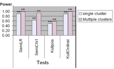
For ordinal categorical data which are generated from the quantized normal II type, Figure 5 shows that the
semiparametric method with the likelihood ratio test has the highest power of detecting potential clusters among all the tests. The semiparametric method with the c1test works well but not as good as the likelihood ratio
test. This is in line with the limited power study in Kedem and Wen (2007) [16] which showed the like-lihood ratio test was the most powerful tests among three tests from the semiparametric density ratio model. Moreover, when the clustering pattern is stronger, for instance, the study region contains multiple clusters, the power ofc1test increases to 0.94, which is almost close
to the power of the likelihood ratio test. The power of Kulldorff’s method with Poisson model is very low, Figure 5
Power comparison between Kulldorff’s and the Semiparametric methods for ordinal categorical data generated from quantized normal II data, where the means are fixed at 13 but the variances are 4 and 8, between the cluster region and the rest of the area, respectively.
Figure 6
because Poisson model is designed to detect the difference in the mean not in the variance. Kulldorff’s method with ordinal model is comparable to the semiparametric method with the c1 test in detecting
potential clusters.
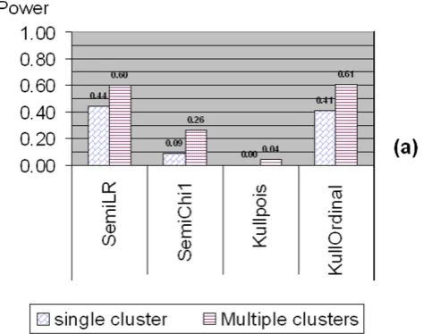
For ordinal categorical data which are generated from the quantized normal III type, Figure 6 shows that the semiparametric method performs in the same way as in the quantized normal II case. The semiparametric method with the likelihood ratio test still has the highest power in both single and multiple clusters situation. The power of all tests increases as the clustering pattern becomes stronger. Kulldorff’s method with the ordinal model performs equally well as compared to
semiparametric method. Kulldorff’s method with Pois-son model“works”but still much less powerful than the other tests. This is because for the quantized normal III data, Kulldorff’s Poisson model can detect the changes in the mean while still ignoring changes in the variance.
The part (a) of Figure 7 shows the power results when the difference (in the mean) between the cluster and non-cluster regions is small. The data are still ordinal categorical data generated from the quantized normal III type. However, this time the difference is that the mean in the cluster region was set to be close to the the non-cluster region, while the variances inside and outside the cluster region were kept the same as in the previous case (refer to Table 2 for the simulation parameters). In this way, the clusters were more difficult to detect. Not surprisingly, the power for the semiparametric method with the likelihood ratio test and Kulldorff’s method with the ordinal model continue achieving the highest power, although it is much lower than the power in the previous case where the differences inside and outside the cluster region were substantial. The power of the c1
test of the semiparametric method also decreases due to the weaker cluster pattern, and Kulldorff’s method with the Poisson model yields the lowest power almost 0. The multiple cluster case is similar to the single cluster case but with a relatively higher power. Interestingly, if we look at the accuracy, which means detecting the true cluster region correctly with its exact size, the most accurate method as shown in the part (b) of Figure 7 is the semiparametric method with the likelihood ratio test statistic, which achieves more than 50% higher accuracy rate than Kulldorff’s method with the ordinal model.
A Case Study—North Humberside childhood leukemia data set
The semiparametric method with Storey’s q-value for adjusting the multiple-testing was again applied to the North Humberside childhood leukemia data set under the same conditions as used in Kedem and Wen (2007) [16]. As shown in Figure 8, both Kulldorff’s method and the semiparametric method point to the same cluster as the primary cluster candidate, but but Kulldorff’s method gave a highly insignificant p-value of 0.674, whereas the semiparametric method gave a significantp -value of 0.002 without adjusting for multiple testing and a close to boundary q-value of 0.073 adjusted by the Storey’s approach. Thus, the results from the semipara-metric method are more in line with the medical and environmental studies of Cuzick et al. (1990), Mckinney et al. (1991), and Colt and Blair (1998), which suggested that the North Humberside region had paternal exposure to solvents which were strongly associated with leukemia [39,41]. It seems the results from the semiparametric Figure 7
method that the located cluster candidate is a true cluster are more credible. More conclusive results may be obtained by increasing the sample size.
Discussion and Conclusion
In this paper, We extended the semiparametric cluster detection method of Kedem and Wen (2007) [16] by incorporating Storey’s q-value method, a type of FDR method, to overcome the multiple-testing problem raised by numerous scan windows of variable size. The results of the power study show that when detecting localized clusters, both the semiparametric and Kull-dorff’s method can achieve comparably good power. For binary population-case data, Kulldorff’s method with Poisson model may have a slightly higher power than the semiparametric method with the tilt functionh(x) = x. We may choose the tilt function ash(x) = (x, x2)’ for binary data as well although thex2term is not necessary. See Appendix 1 for a more detailed explanation. For non-binary data, such as ordinal categorical data, the semiparametric method with the tilt functionh(x) = (x, x2)’ is slightly more powerful than Kulldorff’s method with the ordinal model. If Kulldorff’s method is applied with an inappropriate model, it may fail to detect any potential clusters as shown in the simulation study for non-binary data. We also find that in our semiparametric method the likelihood ratio test seems to have higher power than the c1 test in detecting potential clusters.
When the localized clustering pattern is strong, for instance, multiple cluster regions or the difference inside and outside the cluster region is large, both tests obtain good power. When the clustering pattern is weak, that is, the difference is not that large, the likelihood ratio test
seems to be acuter, while thec1test could be insensitive
to the undesired fluctuations. In addition, the Likelihood ratio test only can test“either high or low values”, butc1
test can be easily transformed into a one-sided test [16] for two-sample comparison and scalar tilt function. In practice, it is prudent to use both tests for potential clusters. Potentially, if one wants to borrow information from other sources besides the current study region, the c2-test of the semiparametric method could be used.
In the power study for non-binary data, we only used the ordinal categorical data, which are integer data, to compare the power of the two methods. However, Kulldorff’s method also provide exponential model to analyze the survival data, which are mostly assumed to be exponentially distributed, and a normal model to analyze continuous data. A future study is to compare the power of the semiparametric method and Kulldorff’s method for continuous data. But we may expect the semiparametric method will still work well, since the semiparametric density ratio model was originated from continuous data. In addition, the semiparametric model may have a more consistent setup than Kulldorff’s method. Kullorff’s method needs to choose different models, namely different scan statistics, for different types of data, whereas the semiparametric method requires no complete distributional assumptions except for the tilt function h(x). It could choose h(x) = (x, x2)’ for many types of data, no matter continuous or discrete.
If the underlying distribution is known exactly, semi-parametric could choose the appropriate tilt function h (x) to get the best performance. For instance, if the data are known from Bernoulli or Poisson distribution, we can use the tilt function h(x) = x; if the data are from normal, we can use h(x) = (x, x2)’; if the data are from Gamma distribution, we can useh(x) = (x;logx)’. A clue of how to choose a satisfactoryh(x) for a given situation can be derived from common exponential families. More examples can be found in Kedem and Wen (2007) or Kay and Little (1987) [16,42]. In addition, Fokianos et. al. (2001) [30] suggested that h(x) could be approxi-mated by a polynomial, B splines, or kernel estimation. If the underlying distribution is not known, there could be a problem of the misspecified tilt function. Fokianos and Kaimi has discussed that a misspecified h(x) could decrease the power of the corresponding tests [43,44]. Yet, there are examples where very different choices ofh (x) could lead to similar test results. For instance, in an application to meteorological data in Kedem et al. (2004) [45] the choice of h(x) = x or h(x) = logx led to very similar results. It seems that for a non-homogeneous regional variance the choice ofh(x) = (x, x2)’suggested by the normal distribution is sensible. Figure 8
The semiparametric density ratio model essentially tests the homogeneity or equidistribution of two or more samples, therefore, besides Kulldorff’s circular scan window, the semiparametric method may also adapt to other shape of the scanning window or scanning schemes, such as the Kulldorff’s elliptic window scan, irregular shape upper-level set scan, or flexible scan, etc. More precisely, in scanning for clusters, and regardless of the regular or irregular shape of the scanning window, as long as the window separates the whole study region into two samples, one inside the window and one outside the window, the semiparametric method can be applied. However, it also makes the semiparametric method ignore the information about the location of the cases except whether the case is inside or outside the current evaluated window. Thus the semiparametric method may not have good power for global type clustering as shown in scenarios 10 to 15 in Figure 3 and 4 where clustering occurs throughout the study region.
A limiting factor of this power study might be that in the power study for non-binary type data we only used 100 runs at one point for each power comparison. That is because it is tedious and time consuming to run SatScan software and document the results manually. In addi-tion, the semiparametric method also takes longer time to numerically estimate the parameters a and b especially when the combined sample size is big, while for binary scan the MLEs of a andb have already been obtained in closed forms. However, although 100-run does not sound like a large number in simulation, the results are still meaningful. From Figures 5 and 6, it is already clear to show the semiparametric method achieves comparable good power as Kulldorff’s method with the correct model achieves. If Kulldorff’s method is applied with an inappropriate model, the power may decrease a lot. Figure 7 demonstrates that when the difference between the cluster and non-cluster region is small, the detecting power for both methods decrease, but the likelihood ratio test from the semiparametric method seems have better accuracy in detecting clusters.
A last note is about the π0 in Storey’sq-value method.
The critical part of theq-value method of controlling the false discovery rate is to give a good estimate of π0, the
proportion of the true null hypotheses among all the tests. The current method we used in this study is based on the algorithm suggested by Storey et al. (2003) [35] and assume the distribution ofp-value from each test is uniform over the (0,1) interval. However, Yang (2004) [46] pointed out that if thep-values were not uniformly distributed, the power of the q-value method may decrease. He suggested to compute a weighted average ofπ0from the distribution of the rawp-values which are
greater than a threshold (say 0.4). Thus it may give a better control and more robust estimate ofπ0.
Appendix 1
—
Simplified Semiparametric Test
Statistics for Binary Data
If the data are 0-1 binary, such as cancer or not cancer, we can simplify the likelihood and obtain closed forms for the estimated parameters. Recall:
NG: The combined sample size for the whole study region.
nG: The number of cases in the whole study region.
NZ: The sample size within the scan window.
nG: The number of cases within the scan window.
ti: Theith observation from the combined sample in the whole study region,i= 1,...,NG.
r1: The relative sample size, which is equal toNZ/(NG -NZ).
xZj: The jth observation within the scan window Z, j = 1,...,NZ.
For binary data, choose the tilt function h(x) =x. Then the profile log-likelihood with parametersa1andb1is
( , ) log[ ] ( )
(
1 1 1
1
1 1
1
1 1 1
e
xN n
t
i N
Zj j
N
G G
i
G Z
)) log
log
1
1
1
1 1
1
N Z NG N Ze
n N Z
NG N Ze N
G Z
n
Z 1
(13)
The resulting maximum likelihood estimators are,
ˆ log log ( ) ( )
ˆ log
1
1
N Z nZ N Z
NG N Z nG nZ NG N Z nZZ
N Z nZ
nG nZ NG N Z nG nZ
e nZ N Z
log
( ) ( )
/ (
ˆ ˆ 1 1
n
nG nZ NG N Z
)/( )
(14)
If b1= 0, it impliesa1= 0 andea1+b1= 1, which means
By equation (7), then c1 test statistic then can be
simplified to
1 1 1
1 1 2
1
N nG nZ
NG N Z
nG nZ NG N Z
G ˆ
( )
( )
ˆ
1
(15)
Where 1 NG N ZN Z and ˆ1 is as in equation (14).
By equation (9), then the likelihood ratio test statistic can be simplified to
LR nZ N Z
nG nZ NG N Z
N Z nZ N Z
nZ nG nZ NZ nZ
2 2
log ( ) ( ) ( )
logg (( ) ( ))
log ( )
( ) ( )
NG N Z nG nZ NG N Z nG
NG
N N n n
n
G Z G Z
G
2
( ) log [ NG nG NG
NG nG
2 Kulldoff’s Bernoulli scan statt. as in equation ( )]1
(16)
If the tilt functionh(x) is chosen as (x,x2)’, the parameter b11 and b12 are associated with the x and x2 term,
respectively. Notice that for 0-1 binary data, x = x2 in value, thus
11 12 2 1
x x x,
the x2 term is confounded with x, and b12 is not
estimable. Therefore, tilt function h(x) = x with para-metersa1,b1are sufficient for binary case.
Appendix 2
—
Derivation of
S, V
The matricesS, Vare derived by repeated differentiation of the log-likelihood (eq. 17), which is the generalized version of equation (4) form samples (m =q+ 1) with themth sample being the reference sample.
( , ) log[ ( ) ( )]
( ( ))
1 1 11
1
w t w t
x
i q q i
i n
i i ij
j n h ii i q
1 (17)Recall that the asymptotic covariance matrix of the estimates in (5) is given by the product
S VS1 1 (18)
First define
1,, q, 1, q (19)
Then E[∇ l(a1,..., aq, b1,..., bq)]=0. To obtain the score
second moments it is convenient to definerm≡1,wm(t) ≡1
Ej[ ( )]ht
h( )t w t dG tj( ) ( ) (20)and,
A j j w j t w j t dG t kwk t k q 0 1 1 ( , ) ( ) ( ) ( ) ( )
(21)A1 h
1 1
( , ) ( ) ( ) ( ) ( ) ( ) j j t w j t w j t dG t
kwk t k
q
(22)A2 h h
1 1
( , ) ( ) ( ) ( ) ( ) ( ) ( ) j j t t w j t w j t dG t
kwk t k
q
(23)forj, j’= 1,...,q. Then, the entries in
V
Var
n l q q
1
1 1
( ,, , ,, ) (24)
are
1 2
1 1 0 0
2 1 nVar l j j k k
q A j j rA j r
r m
{ ( , ) ( , )} (25) 11 1 0
0 nCov l j l j j j k k
q A j j
A j r
r , { ( , )
( , ))A ( , )}j r
r m 0 1
(26) 1 21 1 0
nCov l j l j j k k
q A j j E t
A j r , { ( , ) [ ( )] h 0 0 1 1
( , )j r ( , )}j r
1
1 1 0
nCov l j l j j j k k
q A j j Ej t
, { ( , ) [ ( )
h ]]
( , ) ( , )}
rr m
A0 j r 1 j r 1
A
(28)
1
1 1 2
nCov l j l j j j k k
q j j Ej t , { ( , ) [ ( )
A h ]] ( , ) ( , ) [ ( )] ( , ) ( , )}
A A h A A 1 1 1 1 1 1 j jj j E t
j r j r
n j r r m C
Cov ji j k k
n
i nj j
[ (h ), (h )]
1 1 (29)The last term is 0 forj≠j’and (nj/n)Var[h(∈j1)] forj=j’.
Next, asn!1,
1 1 1
n l( ,,q, ,,q) S (30) where S is a q(1 + p) × q(1 + p) matrix with entries corresponding toj, j’= 1,...,q,
1 2 2 1 1 1 1 1 n l j j k k q kwk t k j q
w j t
kwk t k q d [ ( )] ( ) ( ) G G t( )
(31) 1 2 11 1 1
n l j j j j k k q
w j t w j t kwk t k
q dG t
( ) ( ) ( ) ( )
(32) 1 2 1 1 1 1 n l j j j k k qkwk t w j t t k j q kwk [ ( )] ( ) ( ) ( h tt k
q dG t
) ( )
1 (33) 1 21 1 1 1
n l j j j j k k q
w j t w j t t kwk t k ( ) ( ) ( ) ( ) h q
q dG t
( ) (34) 1 2 1 1 1 1 n l j j j k k q kwk t k j qw j t t t
[ ( )] ( ) ( ) ( )h h
kkwk t k
q ( ) dG t( )
1 (35) 1 21 1 1
n l j j j j k k q
w j t w j t t t kwk t ( ) ( ) ( ) ( ) ( h h )) ( ) k
q dG t
1 (36)Competing interests
The authors declare that they have no competing interests.
Authors
’
contributions
BK proposed the idea to apply the semiparametric density ration model to cluster detection. SW imple-mented the idea and developed the semiparametric cluster detection method. SW wrote the Splus code, conducted the power comparison, and wrote the manu-script. BK gave valuable comments to the manumanu-script. All authors have read and approved the final manuscript.
Acknowledgements
Special thanks to Professor Martin Kulldorff for all of his help during this research. Also thanks for the valuable comments from the three reviewers.
References
1. Pickle LW, Feuer EJ and Edwards BK: U.S. Predicted Cancer Incidence, 1999: Complete Maps by County and State From Spatial Projection Models. National Cancer Institute, Cancer Surveillance Monograph No. 52003, NIH Publication No. 03-5435. 2. Glaz J and Balakrishnan N:Scan Statistics and ApplicationsNew York:
Springer; 1999.
3. Glaz J, Naus J and Wallenstein S:Scan statisticsNew York: Springer; 2001.
4. Naus JI:The distribution of the size of the maximum cluster of points on a line. Journal of the American Statistical Association
1965,60:532–538.
5. Shmueli G and Fienberg SE:Current and potential statistical methods for monitoring multiple data streams for bio-surveillance.Statistical Methods in Counter-Terrorism: Game Theory, Modeling, Syndromic Surveillance, and Biometric Authentication New York: Springer: Wilson A, Wilson G, Olwell DH 2006, 109–140. 6. Patil GP and Taillie C: Upper level set scan statistic for
detecting arbitrarily shaped hotspots. Environmental and Ecological Statistics2004,11:183–197.
7. Patil GP, Rathbun SL, Acharya R, Patankar P and Modarres R:
Geoinformatic surveillance of hotspot detection, prioritiza-tion and early warning. Proceedings of the 2005 National Conference on Digital Government Research2005, 301–302.
8. Modarresa R and Patil GP: Hotspot Detection with Bivariate Data.Journal of Statistical Planning and Inference2007,11:3643–3654. 9. Tango T and Takahashi K:A flexibly shaped spatial scan statistic for detecting clusters.International Journal of Health Geographics
2005,4:11–25.
10. Takahashi K, Kulldorff M, Tango T and Yih K:A flexibly shaped space-time scan statistic for disease outbreak detection and monitoring. International Journal of Health Geographics 2008,
7:14–27.
11. Kulldorff M:A spatial scan statistic.Communication in Statististics: Theory and methods1997,26:1481–1496.
12. Kulldorff M:Spatial scan statistics: models, calculations, and applications. Scan Statistics and Applications Boston: Birkhäuser: Glaz J, Balakrishnan N 1999, 303–322.
13. Kulldorff M:Prospective time periodic geographical disease surveillance using a scan statistic.Journal of the Royal Statistical Society A2001,164(part 1):61–72.
15. Jung I, Kulldorff M and Klassen AC: A spatial scan statistic for ordinal data.Statistics in Medicine2007,26(7):1594–1607. 16. Kedem B and Wen S:Semiparametric cluster detection.Journal
of Statistical Theory and Practice2007,1:49–72.
17. Waller LA and Lawson AB: The power of focused tests to detect disease clustering. Statistics in Medicine 1995,
14:2291–2308.
18. Alexander F, Cartwright R, McKinney PA and J RT:Investigation of spatial clustering of rare diseases: childhood malignancies in North Humberside.Journal of Epidemiology and Community Health
1990,44:39–46.
19. Storey JD:A direct approach to false discovery rates.Journal of the Royal Statistical Society Series B2002,64:479–498.
20. Storey JD: The positive false discovery rate: a bayesian interpretation and the q-value. Annals of Statistics 2003,
31:2013–2035.
21. Benjamini Y and Hochberg Y: Controlling the false discovery rate: a practical and powerful approach to multiple testing. Journal of the Royal Statistical Society Series B1995,57(1):289–300. 22. Kulldorff M, Tango T and Park PJ:Power comparison for disease
clustering tests. Computational Statistics & Data Analysis 2003,
42:665–684.
23. Kulldorff M, Heffernan R, Hartman J, Assunção RM and Mostashari F:
A space-time permutation scan statistic for the early detection of disease outbreaks.PLoS Medicine2005,2:216–224. 24. Dwass M: Modified randomization tests for nonparametric hypotheses. The Annuals of Mathematical Statistics 1957,
28:181–187.
25. Barlow RE, Bartholomew DJ, Bremner JM and Brunk HD:Statistical Inference under Order RestrictionsNew York: Wiley; 1974.
26. Dykstra R, Kochar S and Robertson T:Inference for likelihood ratio ordering in the two-sample problem. Journal of the American Statistical Association1995,90(431):1034–1040.
27. Kulldorff M, Mostashari F, Duczmal L, Yih WK, Kleinman K and Platt R:Multivariate scan statistics for disease surveillance. Statistics in Medicine2007,26(8):1824–1833.
28. Kulldorff M, Huang L and Konty K: A spatial scan statistic for normally distributed data.2009 http://populationmedicine.net/ content/docs/normalscan-posted.pdf.
29. Kulldorff M, Huang L, Pickle L and Duczmal L:An elliptic spatial scan statistic.Statistics in Medicine2007,25(22):3929–3943. 30. Fokianos K, Kedem B, Qin J and Short DA: A semiparametric
approach to the one-way layout.Technometric2001,43:56–65. 31. Qin J and Zhang B:A goodness of fit test for logistic regression models based on case-control data. Biometrika 1997,
84:609–618.
32. Qin J and Lawless JF: Empirical likelihood and general estimating equations.The Annals of Statistics1994,22:300–325. 33. Sen PK and Singer JM:Large sample method in statistics, An introduction
with ApplicationsLondon: Chapman and Hall/CRC; 1993.
34. Reiner A, Yekutieli D and Benjamini Y:Identifying differentially expressed genes using false discovery rate controlling procedures.Bioinformatics2003,19(3):368–375.
35. Storey JD and Tibshirani R:Statistical significance for genome-wide studies.Proceedings of the National Academy of Sciences2003,
100:9440–9445.
36. Tsai C, Hsueh M and Chen J: Estimation of False Discovery Rates in Multiple Testing: Application to Gene Microarray Data.Biometrics2003,59(4):1071–1081.
37. Storey JD, Taylor JE and Siegmund D: Strong control, con-servative point estimation, and simultaneous concon-servative consistency of false discovery rates: A unified approach. Journal of the Royal Statistical Society Series B2004,66:187–205. 38. Gagnon R: Certain Computational Aspects of Power
Effi-ciency and of State Space Models. PhD thesis, University of Maryland, College Park, Department of Mathematics2005.
39. Cuzick J and Edwards R:Spatial clustering for inhomogeneous populations. Journal of the Royal Statistical Society B 1990,
52:73–104.
40. McKinney PA, Alexander FE, Cartwright RA and Parker L:Parental occupations of children with leukemia in west Cumbria, North Humberside, and Gateshead.British Medical Journal1991,
302:681–687.
41. Colt JS and Blair A:Parental Occupational Exposures and Risk of Childhood Cancer. Environmental Health Perspectives Supple-ments1998,106(S3):909–925.
42. Kay R an