Complementarity of Different Approaches for Assessing Vertical Turbulent Exchange Intensity in Natural Stratified Basins

Complimentarity of Different Approaches for Assessing Vertical

Turbulent Exchange Intensity in Natural Stratified Basins

A.S. Samodurov

Marine Hydrophysical Institute, Russian Academy of Sciences, Sevastopol, Russian Federation

e-mail: [email protected]

The comparison of previously proposed theoretical and semi-empirical approaches for assessing dependence of vertical turbulent exchange on stratification in the natural basins is carried out. The following models are compared: the semi-empirical model based on vertical probing data for revealing dependence of the required parameters on the stratification; the theoretical “spectral” model indicating qualitative differences in the exchange parameters in the “strongly” and “weakly” stratified layers of the main pycnocline in natural basins; the 1.5D model of the Black Sea vertical exchange developed within the framework of the inverse problem. The models, being analyzed in the course of calculating dependence of the energy dissipation rate ε and the diffusion coefficient K upon the buoyancy frequency N, show that they do not contradict each other and, if necessary, can complement each other. In addition, it is found that the greatest physical completeness among the considered models contains the “spectral” model that takes into account a variety of possible distributions in the upper “strongly” stratified layer. However, there are certain difficulties with assessment of the relevant coefficients in, dependencies. The latter problem can be solved within the framework of this approach via proper measurements in the investigated area using the semi-empirical approach relationships. A correspondence between the pair of “spectral” model and semi-empirical model and the 1.5D model for the Black Sea, which will be used in the future, should be also noted.

Keywords: internal wave shear instability, energy dissipation, vertical turbulent diffusion, vertical exchange models.

DOI: 10.22449/1573-160X-2016-6-32-42

© 2016, A.S. Samodurov © 2016, Physical Oceanography

Introduction. Manifestations of vertical exchange mechanisms in the stratified layers of natural basins play an important role in the formation and evolution of the structures under observation in the fields of temperature, salinity and dissolved chemical substances. There are a lot of natural contributors to the vertical exchange. In addition to various types of advective transport, density convection, manifestations of double diffusion mechanisms, near-bottom friction, bottom geothermal heat flux and many others are among these contributors. The analysis of accumulated data reveals the fact that shear instability of inertia-gravity internal waves (extremely low-frequency quasi-horizontal and periodical by the depth of currents) accompanied by their local breakings and formation of turbulent mixed spots makes the most significant contribution to the turbulent exchange for the stratified layers on the entire World Ocean scale [1]. A lot of theoretical, semi-empirical and experimental models (represented in the literature) have been created during the study of this exchange mechanism. References to the series of such papers are given in Table 1 as an example.

data [9] based on it revealed that at least two approaches are required in natural stratified layer to describe turbulent diffusion dependence on stratification. Nominally, it should be the following models: the one for lower, “weakly” stratified layer and for upper, “strongly” stratified one in pycnocline. A brief description of our vertical turbulent diffusion models in which the mentioned approaches are taken into account naturally or with a consideration of exchange physical features in different layers. A comparison of the models is also carried out.

T a b l e 1

Relationship of turbulent energy dissipation rate ε with local buoyancy frequency N(z) in different models of vertical turbulent diffusion

Set of models I Set of models II

Authors _{ε ∝} Authors Type of IW

spectrum ε ∝

McComas, Muller [2] 2

N Munk [5] Broadband 3/2

N

Henyey et al. [3] 2

N Gargett, Holloway [6] Broadband 3/2

N

Winters, D’Asaro [4] 2

N Gargett [7] Narrowband N

Semi-empirical model of vertical turbulent diffusion in stratified natural basins. Semi-empirical model [10, 11] was constructed on the basis of data collected during temperature vertical probing in different areas and at different horizons.

hydrologic situation (the upper “strongly” stratified layer). The obtained result is represented by the following relation:

1

−

≅DNc

L m, (1)

where

[ ]

N_c =cycle/h, D≅1,4 m (cycle/h). It should be pointed out that the exponent of buoyancy frequency decreases down to –0.85 in the array of mixed probing data (~200 spectra from different areas and different moderate depths). What for the abyssal data (Fig. 2), it seems that the exponent should change down to zero at minimum values of N,though the data amount is not sufficient enough for statistical analysis. Relation (1) remains the most statistically significant exponential dependence for the upper “strongly” stratified layer.

Fig. 1. Scheme of vertical spectrum of temperature fluctuation gradients in the main thermocline proposed by M. Gregg [12]

Fig. 2. Mean scale of turbulent spot L (analyzed in [10, 11] by the data from moderate depths of the Atlantic Ocean, the Black and the Mediterranean Seas (+), from the upper stratified layer of the Indian Ocean tropical zone (■) and according to abyssal data (▲, ●)) depending on buoyancy frequency local value

the stratified medium is related to the energy losses on the potential energy increase and dissipation. In the formed spot of L thickness and Σ area during its formation the potential energy variation rate Π is as follows:

t L N ∆ Σ = Π 12 3 2 0 ρ  _,

where ρ₀ is a thickness-average density; ∆t is a characteristic time of spot formation. Then, mainly applying a series of laboratory results the desired relationship takes the following form:

3 2 2 10 2 ,

8 ⋅ − LN

≅

ε , (2) and diffusion coefficient is equal to

2

1 R N R K

f

f ε

−

≅ . (3)

Using the results of laboratory experiments [13, 14] and several mechanistic approaches in [15], the constancy of dynamical Richardson number Rf (ratio of

potential energy increase rate in the system to the rate of intake of energy spent on the mixing) in the acts of stratified flux shear instability and breaking of wave perturbations was determined. Several approximate values of Rf (1/3 in [13] and

1/4 in [14]) and 0.2 value for assessment of the entire multiplier of the expression (3) right side in [16] were proposed for application in the calculations.

If we choose 0.25 value for Rf (which was done to draw up the correlation

(2)), we will obtain the following expression for diffusion coefficient:

N L

K≅2,7⋅10−2 2 . (4)

Using empirical result (1) in the expressions (3) and (4) and turning to a cyclic frequencyN_c, we obtain ε(Nc) and K(Nc) distributions for the upper “strongly”

stratified layer at the given value of D coefficient:

c

N

~

10

56

.

8

⋅

−10

≅

ε

m2∙_s−3_,

c

c

N

N

~

=

(cycle/h)−1, (5)

1

5

~

10

36

.

9

⋅

− −

≅

N

c

K

m2∙_s−1_{. (6)}

In the paper [10] it is pointed out that our semi-empirical result (5) (and, consequently, (6)) corresponds well to the result of measurement analysis ε(Nc)in the upper thermocline in the Sargasso Sea near Bermuda and on the continental shelf in the area of British Columbia (Fig. 3) [6].

It should be mentioned that if the abyssal data obtained in “weakly” stratified layers (Fig. 2) (being more numerous) provided L(N)=const relationship, the pair of functions required within the framework of this problem, considering the expressions (2), (4), would be of the form

N K

N ∝

∝ 3,

in contrast to the data for the upper layer (formulas (5) and (6)) where the following expressions are correct:

N

∝

ε , K∝N−1. (8) The possibility of getting the result (7) is rather high. For instance, in our recent paper [17] it was determined that such situation (reliable assessment of

≅

) (N

L const for small N) was observed in late autumn in the Black Sea near-surface “weakly” stratified layer. There was also drawn a conclusion that the situation (7) depends on stratification features (here – the “weak” one), not on the layer localization by depth.

Fig. 3. Ensemble-averaged values of kinetic energy ε dissipation rate depending on N from the paper [6] (squares). Straight line corresponds to expression (5)

c n

wd w

n k

QN dn E E e

c min

2

)

( − =π

=

∆

∫

∞

. (9)

Here the model vertical spectra without and with losses for energy dissipation, as well as energy dissipation rate, have the following form, respectively [8]:

2

min 2

2 −

= n

k QN Enw

π

, n≤n_c; _nwd n n_c k

QN

E 3

min 2

2 −

= π , n≥n_c; ε =∆e/∆t.

In the given relationsQis spectrum level, k and n are horizontal and vertical wave numbers, respectively. According to experimental approach in [18], the time spent on the formation of turbulent spot is equal to∆t≅4/N. In this case, the assessment for energy dissipation rate is calculated as

3

min

4k n N Q

c

π

ε ≅ . (10)

c

Qn k

πmin

Ri_Σ ≅ . (11)

We emphasize that buoyancy frequency N is not obviously included in the right part of (11). Now we are to consider its role in the structure of critical scale nc

which was discussed in [8]. The region of existence of internal waves in k, n

coordinates with one of possible nc positions on n axis is schematically

represented in Fig. 4, a. Critical frequency which is close to f inertial one has the following form at that (through the dispersion relationship):

2 2 min 2 2 2

c c

n k N f +

≅

ω , ωc2 <<N2,

2 2

min nc

k << . (12)

Fig. 4. The areas of quasi-inertial internal wave energy loss (darkened) according to model [8] for “weakly” stratified (1 in fragment a) and “strongly” stratified (2 in fragment b) layers

In Fig. 4 shaded areas correspond to energy loss areas. Vertical spectra calculated according to the measurements carried out in the main pycnocline indicate (Fig. 1) that break area l makes up ~10 m on the spectrum [6, 12, 19 and others]. This value is an order of magnitude less than the maximum permissible value of λmax =2π/nminwave scale in the mentioned layer within the framework of

WKB approximation applied in the model. If, as is shown by the measurements, shear flows near λmaxscale (or wave number nmin) are stable according to

Richardson criterion, the instability for formation in the area spectrum with energy losses is implemented on smaller scales with 2π/ncupper boundary (Fig. 4, a)

(which does not depend on N (formula (11))) and ωc frequency (formula (12)).

Thus, as it was revealed by the analysis, the considered situation describes the structure of the main pycnocline lower part and required functions (according to relations (10) and (3)) correspond to the following dependences on N :

N K

N ∝

∝ 3,

ε . (13)

ω

n

min

n

c

k

kmin

n

ω

_c

ω

1

k

kmin

n

c

=n

min

n

ω

c

2

When considering the situation in the upper part of the main pycnocline, at first we should notice that the restrictions may be imposed upon λ_max =2π/n_minscale. These restrictions are related to the fact that vertical scale of a wave must be much smaller than the characteristic scale of buoyancy frequency variation. Then, the following relationship is correct for the wave number nmin:

0

min N/ z/N

n >> ∂ ∂ , (14)

where N0 is some characteristic value of buoyancy frequency in the layer under

study.

It should be pointed out that if we exclude a variant of purely linear approximation of distributionN(z), the absolute value of ∂N/∂z derivative in the layer under consideration will increase with a depth reduction. Then, the value

min

n should also increase with a depth reduction in order to satisfy the condition (14). The situation when this value increases and becomes equal to critical scale nc

(Fig. 4, b) is rather probable at that. Upon the further depth decrease, this critical scale will increase along with nmin scale increase in accordance with buoyancy

frequency derivative distribution over depth. It must be said that the mentioned

min

n scale variation also occurs in the main pycnocline lower part but, firstly, this process is rather slow and, secondly, critical vertical scale remains constant (~10 m, Fig. 1) until it becomes equal to decreasing scale 2π/n_minat higher horizons. Eventually, considering the relations (10), (14) and (3) we have the following dependences on stratification for the required functions:

1 3

/∂ −

∂

∝N N z

ε , K∝N∂N/∂z−1. (15)

When analyzing monotonically decreasing with depth measurement data of buoyancy frequencyN, it is convenient to use for its approximationN∝z−α,

1

≥

α exponential function that provides the following dependence of ε energy dissipation rate onα:

α β

ε

_{∝ =} 2−1/

N

N , or β =2−1/α . (16)

In the paper [9], where the analysis of high number of probing data and calculations of required functions (ε and N) in different areas of the ocean was carried out, a reliable correspondence to the model expressions (13) in the main pycnocline as well as to model expressions for ε from (15) in the upper stratified layer in 1≤β<2 scale range was found. It should be pointed out that

) (N

K dependence in this layer amounts to the following expression:

( )

z z

N

K∝ −1/α = −α −1α = .

For the exponential function N∝z−1 (most common for the measurements carried out in this layer) relations (15) take the following form:

N

∝

A one-and-a-half dimensional model (1.5D) of vertical turbulent diffusion in the stratified region of the Black Sea. The first such vertical exchange model for the Black Sea which (the one that included vertical advection and vertical turbulent diffusion) was constructed by us in [20, 21].Subsequently, in [22] as well as in the mentioned papers probing data collected over 70 years was applied. A change of basin area with depth was taken into account in the model and temperature and salinity profiles were somewhat corrected at that. A technique of calculation of Kdiffusion coefficient distribution over the depth on average for the entire measurement period is presented in [20, 21]. It should be noticed that unlike the paper [22] where on the basis of the modified database the problem was solved for Cold Intermediate Layer only, the required functions are calculated down to 750 m horizon here.

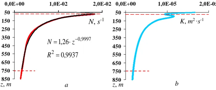
Average over 70 years buoyancy distributions over the frequency N and the diffusion coefficient K are represented in Fig. 5. First of all, it should be pointed out that exponential approximation for buoyancy frequency has N∝z−1 form for the entire range of depths from the maximum Ndown to 750 m (i.e. not just for the upper layer but also for the lower “weakly” stratified one). The same N

( )

z

distribution was previously noted as the one also typical for deepwater parts of the ocean [23].

Fig. 5. Average over 70 years N(z) buoyancy frequency distribution over the depth in the Black Sea (exponential approximation of initial relation) – a; K(z) model relation – b. Red dashed lines denote the depth of N maximum location and the maximum depth down to which the model is valid

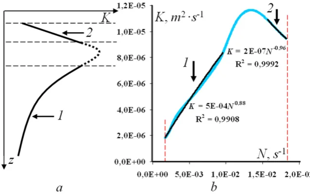
In Fig. 6 a scheme of K(z) vertical distribution (fragment a) and the main result of this section – diffusion coefficient K dependence on buoyancy frequency (fragment b) are given. Black lines correspond to exponential approximations of

) (N

K distribution in lower and upper layers under study. The presence of transition zone probably indicates the fact that exchange mechanisms in it (as well as, for instance, in the zone of buoyancy frequency maximum) are more complex than the ones in the layers under study. The results of comparison of the models constructed by us (which, referring to a single key mechanism of diffusion, are based on different approach to the problem) are given below.

50 150 250

350 450 550 650 750

850

0,0E+00 1,0E-02 2,0E-02

50

150 250 350

450 550

650 750

850

0,0E+00 1,0E-05 2,0E-05

z, m

K, m2 ∙_s-1

N

,

s

-1

9937

,

0

26

,

1

2

9997 , 0

=

⋅

=

−

R

z

N

Fig. 6. Schematic vertical turbulent diffusion coefficient dependence on depth – a and model dependence K(N) – b corresponding to K(z) dependence in Fig. 5, b. Black lines are exponential approximations of model distribution in 1 and 2 layers which, in their turn, correspond to 1 and 2

layers with K(z) solid lines in the fragment a

Conclusions. For the convenience of comparison of the described vertical exchange models we give Table 2 which contains general results. In the first column the analyzed models are given, other three ones contain modeling results for the layers under study. It is obvious that these results do not contradict each other. For instance, in the first column qualitative (with no multipliers) K(N) dependence which is almost similar for the second and the third models is observed. What for the semi-empirical model, there were not enough measurement data in low frequency range Nfor the statistical analysis (in the first section and in the end of this paragraph the arguments for matching of all K(N)dependences are given). In the third column a full compliance of dependences with regard to the overall average dependence N ∝z−1 takes place. The fourth column is given to demonstrate the fact that when analyzing the measurement data in the near-surface “weakly” stratified layer K∝N dependence was revealed. This corresponds to hydrophysical analogy with the lower layer [17].

T a b l e 2

Dependence of vertical turbulent diffusion coefficient K on buoyancy frequency N in the vertical exchange models constructed by us (for the

situations when N∝z-1 _{in the upper layer)} Model

Lower layer,

“weak” stratification

Upper layer, «strong» stratification

Upper layer,

“weak” stratification

Semi-empirical Probably, K∝N _K∝N−1 K∝N

“Spectral” K∝N _K∝N−1_{, ∝} −1

z

N –

1.5D-model, BS _K∝_N0.88≅_{N ∝} −0.96_≅ −1

N N

K –

N o t e: BS – The Black Sea.

Acknowledgements. The research was performed within the framework of the state order No. 0827-2014-0010 “Complex interdisciplinary research of oceanographic processes determining the functioning and evolution of the Black Sea and the Sea of Azov ecosystems on the basis of modern marine environment condition monitoring methods and grid technologies”, and partially with the financial support of RFBR, grant No. 15-05-00984.

REFERENCES

1. Wunsch, C., Ferrari, R., 2004, “Vertical mixing, energy, and the general circulation of the ocean”, Ann. Rev. Fluid Mech., vol. 36, pp. 281-314.

2. McComas, C.H., Muller, P., 1981, “The dynamic balance of internal waves”, J. Phys. Oceanogr., vol. 11, pp. 970-986.

3. Henyey, F.S., Wright, J. & Flatte, S.M., 1986, “Energy and action flow through the internal wave field: An eikonal approach”, J. Geoph. Res., vol. 91, pp. 8487-8495.

4. Winters, K.B., D’Asaro, E.A., 1998, “Direct simulation of internal wave energy transfer”, J. Phys. Oceanogr., vol. 27, pp. 1937-1945.

5. Munk, W., 1981, “Internal waves and small-scale processes”, Evolution of Physical Oceanography, The MIT Press, pp. 264-291.

6. Gargett, A.E., Holloway, G., 1984,“Dissipation and diffusion by internal wave breaking”, J. Mar. Res., vol. 42, no. 1, pp. 15-27.

7. Gargett, A.E., 1984, “Vertical eddy diffusivity in the ocean interior”, J. Mar. Res., pp. 359-393.

9. Samodurov, A.S., Globina, L.V., 2012, “Zavisimost' skorosti dissipatsii turbulentnoy energii i vertikal'nogo obmena ot stratifikatsii po obobshchennym eksperimental'nym dannym (sravnenie s sushchestvuyushchimi modelyami) [Dependence of turbulent energy and vertical exchange dissipation rate on stratification according to experimental data (comparison with the existing models)]”, Morskoy gidrofizicheskiy zhurnal, no. 6, pp. 17-34 (in Russian).

10. Samodurov, A.S., Lyubitskiy, A.A. & Panteleev, N.A., 1994, “Vklad oprokidyvayushchikhsya vnutrennikh voln v strukturoobrazovanie, dissipatsiyu energii i vertikal'nuyu diffuziyu v okeane [Breaking wave contribution to the structuring, energy dissipation and vertical diffusion in the ocean]”, Morskoy gidrofizicheskiy zhurnal, no. 3, pp. 14-27 (in Russian).

11. Samodurov, A.S., Ivanov, L.I., 2003, “Mixing and energy dissipation rate in Mediterranean seas: an intercomparison of existing models”, Oceanography of the Eastern Mediterranean and Black Sea, Similarities and differences in two interconnected basins, Ankara, Tübitak Publishers, pp. 369-375.

12. Gregg, M.C., 1977, “Variations in the intensity of small-scale mixing in the main thermocline”, J. Phys. Oceanogr., vol. 7, no. 3, pp. 436-454.

13. Thorpe, S.A., 1973, “Experiments of instability and turbulence in a stratified shear flow”, J. Fluid Mech., vol. 6, pp. 731-751.

14. McEwen, A.D., 1983, “The kinematics of stratified mixing through internal wave breaking”,

J. Fluid Mech.,vol. 128, pp. 47-57.

15. McEwen, A.D., 1983, “Internal mixing in stratified fluids”, J. Fluid Mech., p. 59-80.

16. Osborn, T.R., 1980, “Estimations of local rate of vertical diffusion from dissipation measurements”, J. Phys. Oceanogr., vol. 10, no. 1, pp. 83-89.

17. Samodurov, A.S., Chukharev, A.M. & Kul'sha, O.E., 2002, “Rezhimy vertikal'nogo turbulentnogo obmena v verkhnem stratifitsirovannom sloe Chernogo morya v rayone Gerakleyskogo poluostrova

[Regimes of vertical turbulent exchange in the Black Sea upper stratified layer near Heracleian Peninsula]”, Protsessy v geosredakh, no. 3, pp. 63-69 (in Russian).

18. Fernando, H.J.S., 1989, “Oceanographic implications of laboratory experiments on diffusive interfaces”, J. Phys. Oceanogr., vol. 19, pp. 1707-1715.

19. Gregg, M.C., “Scaling turbulent dissipation in the thermocline”, J. Geophys. Res., vol. 94, no. C7, pp. 9686-9698.

20. Ivanov, L.I., Samodurov, A.S., 2001, “The role of lateral fluxes in ventilation of the Black Sea”, J. Mar. Syst., vol. 31/1-3, pp. 159-174.

21. Samodurov, A.S., Ivanov, L.I., 2002, “Balansovaya model' dlya rascheta srednikh vertikal'nykh potokov zhidkosti, tepla, soli i rastvorennykh khimicheskikh veshchestv v termokhalokline Chernogo morya [Balance model for calculation of average vertical liquid fluxes, heat, salt and dissolved chemical substances in the Black Sea thermo-halocline]”,

Morskoy gidrofizicheskiy zhurnal, no. 1, pp.7-24 (in Russian).

22. Samodurov, A.S., Ivanov, V.A. & Belokopytov, V.N. [et al.], 2016, “Model' srednegodovogo vertikal'nogo obmena v kholodnom promezhutochnom sloe Chernogo morya [Model of annual average vertical exchange in Cold Intermediate Layer of the Black Sea]”, Protsessy v geosredakh, no. 2(6), pp. 141-147 (in Russian).

23. Monin, A.S., Neyman, V.G. & Filyushkin, B.N., 1970, “O stratifikatsii plotnosti v okeane