www.geosci-model-dev.net/8/3199/2015/ doi:10.5194/gmd-8-3199-2015
© Author(s) 2015. CC Attribution 3.0 License.
A new sub-grid surface mass balance and flux model for
continental-scale ice sheet modelling: testing and last glacial cycle
K. Le Morzadec1, L. Tarasov1, M. Morlighem2, and H. Seroussi3
1Department of Physics and Physical Oceanography, Memorial University of Newfoundland, St. John’s, Newfoundland, Canada
2Department of Earth System Science, University of California, Irvine, California, USA 3Jet Propulsion Laboratory, California Institute of Technology, Pasadena, California, USA Correspondence to: L. Tarasov ([email protected])
Received: 3 March 2015 – Published in Geosci. Model Dev. Discuss.: 1 April 2015 Revised: 16 September 2015 – Accepted: 22 September 2015 – Published: 8 October 2015
Abstract. To investigate ice sheet evolution over the timescale of a glacial cycle, 3-D ice sheet models (ISMs) are typically run at “coarse” grid resolutions (10–50 km) that do not resolve individual mountains. This will introduce to-date unquantified errors in sub-grid (SG) transport, accumulation and ablation for regions of rough topography. In the past, synthetic hypsometric curves, a statistical summary of the topography, have been used in ISMs to describe the variabil-ity of these processes. However, there has yet to be detailed uncertainty analysis of this approach.
We develop a new flow line SG model for embedding in coarse resolution models. A 1 km resolution digital elevation model was used to compute the local hypsometric curve for each coarse grid (CG) cell and to determine local parameters to represent the hypsometric bins’ slopes and widths. The 1-D mass transport for the SG model is computed with the shallow ice approximation. We test this model against sim-ulations from the 3-D Ice Sheet System Model (ISSM) run at 1 km grid resolution. Results show that none of the alter-native parameterizations explored were able to adequately capture SG surface mass balance and flux processes. Via glacial cycle ensemble results for North America, we quan-tify the impact of SG model coupling in an ISM. We show that SG process representation and associated parametric un-certainties, related to the exchange of ice between the SG and CG cells, can have significant (up to 35 m eustatic sea level equivalent for the North American ice complex) impact on modelled ice sheet evolution.
1 Introduction
The resolution used in any model of complex environmen-tal systems (e.g. ice sheet models (ISMs), general circula-tion models or hydrological models) limits the processes that can be represented. For continental-scale glacial cycle con-texts, ISMs are currently run at resolutions of about 10– 50 km (Pollard and DeConto, 2012; Tarasov et al., 2012; Colleoni et al., 2014). Processes such as surface mass bal-ance on mountain peaks, iceberg calving, and ice dynamics in fjords are sensitive to scales of about 100 m to a few kilo-metres and therefore have to be parameterized. For example, even at 10 km grid resolution, mountain peaks are smoothed to bumps in a plateau (Payne and Sugden, 1990), inducing er-rors in computed surface mass balance (Marshall and Clarke, 1999; Franco et al., 2012). If the mean surface elevation of a coarse grid cell is below the equilibrium line altitude (ELA), ice ablation is overestimated (e.g. Tarasov and Peltier, 1997). Thus, coarser grid resolution can lead to temporal and spatial errors in ice sheet inception (Abe-Ouchi and Blatter, 1993; Abe-Ouchi et al., 2013) and subsequent evolution (Van den Berg et al., 2006; Durand et al., 2011).
ex-ample, to improve surface mass balance in continental-scale ice sheet models, Marshall and Clarke (1999) used hypso-metric curves, which represent the cumulative distribution function of the surface elevation. In this method, each indi-vidual glacier is not explicitly represented. Instead, 2-D topo-graphic regions are parameterized with different hypsometric bins, representing a discrete number of elevations and their associated area. In addition to ablation and accumulation at each SG bin, there is SG ice transport from high elevation re-gions to valleys where the average altitude is below the ELA. Starting with ice-free conditions, Marshall and Clarke (1999) found an increase in the total ice volume over North America after a 3 kyr1simulation when this hypsometric parameteri-zation is coupled to an ice sheet model. The impact and ac-curacy of this SG model have yet to be quantified. The model was only validated against observations of a glacier located in the region used for tuning the parameterization (Marshall et al., 2011). Moreover, the communication between the SG and coarse grid (CG) models was identified as a potentially important source of error (Marshall and Clarke, 1999), but its impact has not been documented.
In this paper, we develop a new SG model extending the approach of Marshall and Clarke (1999) and Marshall et al. (2011). We use hypsometric curves that account for a much larger set of topographic information than just the maximum, minimum and median elevation. We present a new slope pa-rameterization to compute the velocities that account for SG slope statistics. An effective width is added for the represen-tation of the ice fluxes between SG bins. In contrast to the one-way communication used in the past, another modifica-tion to the original model is a two-way exchange of ice be-tween the SG and CG cells. The CG ice thickness updating accounts for SG ice thickness, and the SG model accounts for ice flux out of the CG cell. For the first time, we evaluate the accuracy of the SG model against high resolution sim-ulations by a higher order ice sheet model (ISSM; Larour et al., 2012). Sensitivities to the SG model configuration, such as the number of hypsometric bins, are assessed. We examine the extent to which the inclusion of further topo-graphic statistics (e.g. the peak density in a region or the vari-ance of the slopes) can improve computed sub-grid fluxes. We also evaluate the impact of embedding the SG model in the Glacial Systems Model (GSM, formerly the MUNGSM), our coarse grid model, for last glacial cycle simulations of the North American ice complex, using an ensemble of pa-rameter vectors from a past calibration of the GSM (Tarasov et al., 2012). Special attention is given to the impact of the coupling between the SG model and the GSM.
1In this paper, “kyr” is used to represent time intervals and “ka” for time before present day.
2 Model description 2.1 Sub-grid model
The sub-grid model is a finite difference flow line model composed of a diagnostic equation for the ice velocities and a prognostic equation for ice thickness evolution. The surface mass balance is calculated using a positive degree day (PDD) method. The elevation of a 3-D region is parameterized using a hypsometric curve. Differences between the new SG model and the Marshall et al. (2011) approach are summarized in Table 1.
2.1.1 Hypsometric curves
Marshall and Clarke (1999) built their hypsometric curves, representing the basal elevation of a region, synthetically from the minimum, maximum and median elevation of the topography. We generate the hypsometric curves from the GEBCO (General Bathymetric Chart of the Oceans) 1 km resolution digital elevation model (DEM) (BODC, 2010). To select a region fitting the coarse resolution grid cell of the GSM (degrees), the GEBCO Cartesian coordinates are con-verted in degrees assuming the Earth as a perfect sphere with radius of 6370 km. The curves are obtained in a two-step pro-cess. First, the region is divided intoNbins of equal altitude range. Then, to avoid empty bins, the surface elevation range of each empty bin is expanded (consequently decreasing the elevation ranges of the higher and lower adjacent bins) us-ing as many adjacent bins as necessary until these bins rep-resent approximately the same surface area. This process is repeated from the highest bin to the lowest as many times as necessary.
We use 1 km resolution gridded data, so that the area of each bin is proportional to the number of high resolution grid cells assigned to that bin. The alternative of using equal ar-eas in each bin has been discarded as it smooths the results in regions of low peak density. A total of 10 bins have been se-lected in this study, based on the comparison against high res-olution modelling (see Sect. 3.1). Marshall and Clarke (1999) and Marshall (2002) used, respectively, 10 and 16 hypsomet-ric bins in their hypsomethypsomet-ric curves.
At any time step,t, the surface slopes,Skt, for SG bink, from 1 (highest) toN (lowest), are computed from the sur-face elevationhtd,kand an effective lengthLk:
Skt=h t d,k−h
t d,k+1 Lk
. (1)
To compute the slope at the lowest bin we assume an ice cliff boundary condition. The surface elevationhd,N+1is set to the basal elevation of the lowest hypsometric binhb,N.
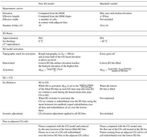
Table 1. Differences between our new SG model and the Marshall and Clarke (1999)/Marshall et al. (2011) models.
New SG model Marshall’s model
Hypsometric curves
Elevation Computed from the DEM Min, max and median elevation Effective lengths Computed from the DEM slopes ∝50 km
Effective width ∝number of cells Not included in contact with adjacent bins
Number of bins (N) 10 10 to 16
SG fluxes
Approximation SIA SIA
Ice rheology 0◦C −40◦C
(T◦equivalence) SG model activation
Topographic mask for activation Rough topography (1 hb>500 m) Every grid cell
and at least half of the CG basal elevation is above sea level
Deactivated Lowest SG bin surface elevation reaches Lowest SG bin filled the bedrock elevation of the highest bin
Activation HCG<hb,SG(top) −hb,CG
2 HCG<
hb,SG(top)−hb,SG(bottom) number of SG bins
SGCG
Ice thickness SG to CG:
While SG is activated,HCGis set to thetotal ice volumeCG cell area When the lowest
of the filled SG bins at each CG time step (the total SG SG bin is filled ice volume is used during the deactivation time step)
CG to SG:
When SG switches to activated, the Not explained CG ice volume is redistributed over the SG bins using the
mean between two methods (equal redistribution over all bins and redistribution of ice over the lowest bins)
Isostatic adjustment CG elevation adjustment applied to all SG bins Not included
Flux to adjacent CG cells
Fluxes computed with the CG model and reduced Fluxes computed with the CG model only by the area fraction of the lowest filled SG bins No flux out of the CG cell treated at the SG level Fluxes in or out of a CG cell redistributed Fluxes coming from an adjacent CG cell to a SG over the lowest SG bins in the adjacent CG cell(s) cell redistributed over the lowest SG bin
Specifically, for each hypsometric bin we compute the slope, Sk0, as the cube root of the mean of the cube of the magnitude of the slopes from the GEBCO data. The effective length,Lk,
for SG binkis computed from the basal elevationhb,k:
Lk=
(hb,k−hb,k+1)
Sk0 , (2)
where hb is the basal elevation. As no information is ex-tracted about the basal elevation downstream of the terminal SG cell, the effective length at the first upstream bin is used at the lowest hypsometric bin. A small effective length can generate unrealistically high velocities in that bin. To avoid this, the lowest bin effective length is set to the mean
effec-tive length of all the hypsometric bins when the altitude dif-ference between the two lowest bins is less than 50 m.
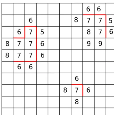
The flow line model requires an effective width,W, for the representation of flux between hypsometric bins.Wk of each
hypsometric bin is set to the total contact length of the SG cells assigned to the bin with adjacent lower hypsometric bin grid cells as detailed in Fig. 1.
2.1.2 Surface mass balance
7 6
8
7
7
7
8
7
7
7
7
7
6
6
6
6
8
8
6
6
5
6
8
9 9
6
5
6
6
8
Figure 1. Schematic representation of the effective width of the 7th
hypsometric bin for a region of 10 km by 10 km. Each square rep-resents a high resolution (1 km) grid cell. The numbers define the hypsometric bin these SG grid cells belong to. The total length of all red lines (14 km) represents the effective width for the 7th bin.
ice surface elevation. A parameterization of the elevation– desertification effect (Budd and Smith, 1981) reduces the precipitation by a factor of 2 for every kilometre increase in elevation. Snow is melted first and the remaining positive de-gree days are used to melt ice with allowance for the forma-tion of superimposed ice. The Supplement includes a more detailed description of the surface mass balance module.
The GSM and ISSM compute the surface mass balance using the same PDD method.
2.1.3 Ice thickness evolution
The prognostic equation for the ice thickness (H) is com-puted, at each hypsometric bin, from the vertically integrated continuity equation as
∂H
∂t = ˙Ms− ∇ ·(uH )= ˙Ms+ ∇ ·(DS). (3) S is the surface slope andM˙s is the surface mass balance rate (basal melt is computed in the CG GSM but ignored in the SG model).uis the vertically integrated ice velocity of the SG model derived using the shallow ice approximation (SIA). The effective diffusivityDis given by
D= 2
n+2(ρg)
nA
0Hn+2(S)n−1. (4)
The creep exponentn of Glen’s flow law is set to 3.A0 is the creep parameter in Pa−3s−1, ρ=910 kg m−3 and g= 9.81 m s−2. Ice flow is insignificant when the ice thickness is on the order of 10 m. To avoid potential numerical instabili-ties, velocity is set to 0 if ice thickness is less than 20 m.
In their most recent experiments, Marshall et al. (2011) tuned their revised model against the present day total ice volume (encompassing 27 % uncertainties) in the eastern slopes of the Canadian Rockies. This tuning sets the ice rhe-ology parameter for an ice temperature equivalence of ap-proximately−40◦C. As the SG model is used for regions that are either starting to accumulate ice or else deglaciat-ing, basal ice temperature (where most deformation occurs) is likely close to freezing. The creep parameter is therefore fixed to a value corresponding to an ice temperature of 0◦C using the Arrhenius relation from the EISMINT (European Ice Sheet Modelling Initiative) project (Payne et al., 2000).
Equation (3) is solved semi-implicitly using a central dif-ference discretization as
1xk1yk
1t
Hkt+1−Hkt=
+Dkthtb,k+Hkt+1−htb,k+1−Hkt++111yk 1xk
− (5)
Dkt−1htb,k−1+Hkt−+11−htb,k−Hkt+11yk−1 1xk−1
+ ˙Ms1xk1yk.
The superscriptstandt+1 represent respectively the current and the subsequent time step.1xis the effective lengthLand 1yis the effective widthWdefined in Sect. 2.1.1.
At the highest bin, we assume that no ice flows into the region. At the lowest bin ice is allowed to flow out of the region.
2.1.4 Model limitations
The shallow ice approximation, used to compute fluxes, is formally invalid for high surface slopes such as present in mountain ranges like the Rockies. Simulating ice evolution over a 3-D terrain using a flow line model limits the ice flow representation. Ice flows from one SG bin to another using an average slope. Our model configuration does not allow for ice at high elevations to flow into an adjacent coarse grid cell. Nor does it allow for ice present at low elevations, in isolated regions having a closed drainage basin, to stay in a coarse grid cell. Moreover, the Arrhenius coefficient is com-puted with a constant ice temperature of 0◦C. High veloc-ities processes, such as periodical surges (Tangborn, 2013; Clarke, 1987), cannot be represented since basal sliding and basal hydrology are not present in the current study.
The hypsometric length parameterization inferred from the surface slopes are correct for ice free regions, but it is only an approximation once the ice starts building up. At the low-est hypsometric bin, slopes are computed assuming ice cliff boundary conditions.
high Arctic report seasonal changes in the surface tempera-ture lapse rates over mountain regions and glaciers, with a mean annual value of about 3.7–5.3◦C km−1(Marshall and Losic, 2011). Rates as low as 2◦C km−1are measured in the summer (Gardner et al., 2009). These values are tested in the GSM ensemble simulations where the lapse rate ranges be-tween 4 and 8◦C km−1.
2.2 GSM
The core of the GSM is a 3-D thermomechanically coupled ice sheet model. The model incorporates sub-glacial tem-peratures, basal dynamics, a visco-elastic bedrock response, climate forcing, surface mass balance, a surface drainage solver, ice calving and margin forcing. The grid resolution used for this study is 1.0◦longitude by 0.5◦latitude.
The thermomechanically coupled ice sheet model, de-scribed in detail in Tarasov and Peltier (2002), uses the verti-cally integrated continuity equation and computes the 3-D ice temperature field from the conservation of energy, taking into account 3-D advection, vertical diffusion, deformation heat-ing, and heating due to basal motion. Velocities are derived from the SIA equations. The sub-glacial temperature field is computed with a 1-D vertical heat diffusion bedrock ther-mal model that spans a depth of 3 km (Tarasov and Peltier, 2007). If the base of the ice is at the pressure melting point, basal motion is assumed to be proportional to a power of the driving stress. The exponent for this Weertman-type power law is set to 3 for basal sliding and 1 for till deformation (detailed description in Tarasov and Peltier, 2002, 2004). The geographic location of the sediment cover is determined from different data sets (Laske and Masters, 1997; Fulton, 1995; Josenhans and Zevenhuizen, 1990). Ice shelf flow is approximated with a linear function of the gravitational driv-ing stress. At the base, ice melt is also computed from the energy balance.
The visco-elastic bedrock response is asynchronously cou-pled to the GSM with a 100-year interval. This module is based on the complete linear visco-elastic field theory for a Maxwell model of the Earth (Tarasov and Peltier, 2002, 2007).
At the surface, the parameterized climate forcing (Tarasov and Peltier, 2004, 2006, 2007) is based on a linear interpo-lation between the present day climatology, derived from a 14-year average (1982–1995) of the 2 m monthly mean re-analysis; Kalnay et al., 1996), and a last glacial maximum (LGM) climatology. The LGM climatology field is derived from a linear combination of PMIP (Paleoclimate Modelling Intercomparison Project)I and II general circulation model results with the linear combination dependent on the maxi-mum elevation of the Keewatin ice dome (PMIP I boundary conditions lacked a major Keewatin ice dome, while PMIP II had a large dome). The interpolation follows a glacial index derived from the GRIP (Greenland Ice-core Project) δ18O record at the summit of the Greenland ice sheet
(Dans-gaard et al., 1993; World Data Center-A for Paleoclimatol-ogy, 1997). The surface mass balance is derived from this climatology using the same methodology as described in Sect. 2.1.2. A surface drainage solver is fully coupled asyn-chronously at 100-year time steps. It diagnostically com-putes downslope drainage, filling any depressions (lakes) if drainage permits (Tarasov and Peltier, 2005, 2006).
The calving module, described in detail in Tarasov and Peltier (2004), is based on a height above buoyancy crite-rion with added mean summer sea surface temperature de-pendence. The inhibition of calving due to the presence of landfast sea ice is also parameterized. To reduce misfits be-tween the model results and geological evidences of the ice configuration, the mass-balance forcing is nudged to pro-mote compliance with geologically inferred deglacial margin chronologies (Tarasov and Peltier, 2004).
2.3 GSM and sub-grid model coupling
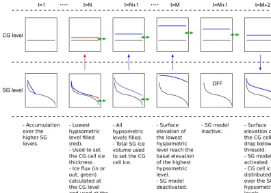
In this section, we describe how the SG model is embedded in the GSM and the conditions applied to activate or deacti-vate the SG model in each CG cell. The GSM is run, at all times, over all the CG cells and the ice thickness is updated in cases where the SG model is activated. Figure 2 gives a summary diagram of the coupling between the GSM and the SG model.
2.3.1 Interaction between the sub-grid model and the GSM
There is two-way communication between the GSM and SG models to exchange information about ice thickness, surface mass balance, and surface temperature. Ice in a CG cell is added to the SG level2 when the SG model switches from deactivated to activated for a given CG cell. The information about the ice evolution at the SG level is used to update the ice thickness, surface mass balance rate and surface temper-ature at the CG level.
CG level
SG level
t=1
....
t=N t=N+1....
t=M t=M+1 t=M+2- Accumulation over the higher SG levels.
- Lowest hypsometric level filled (red). - Used to set the CG cell ice thickness . - Ice flux (in or out, green) calculated at the CG level and used at the SG level.
- All hypsometric levels filled. - Total SG ice volume used to set the CG cell ice.
- Surface elevation of the lowest hyspometric level reach the basal elevation of the highest hypsometric level. - SG model deactivated.
- SG model inactive.
- Surface elevation of the CG cell drop below a thresold. - SG model re-activated. - CG cell ice distributed over the SG hypsometric levels.
OFF
Figure 2. Communication between the GSM and the SG model for one CG cell.
deactivated, the total SG ice volume is transferred to the CG cell.
Once the SG model is reactivated in a CG cell during deglaciation, the ice volume present at the CG level is dis-tributed over the different hypsometric bins. To account for the higher volume of ice in valleys, represented by the low-est hypsometric bins, the average of the following two mass-conserving distributions is used for SG initialization. The first is even distribution across every bin. The second keeps equal surface elevation for the lowest bins, starting from the lowest bin and using as many bins as necessary.
Marshall and Clarke (1999) have no ice flux to adjacent CG cells when the SG model is active. In our model, ice transport between CG cells, computed with the GSM, is modified using SG information. We assume that only the ice present in the filled bins flows out of the coarse grid region; therefore, only a fraction of the CG flux is permitted. This fraction is computed as the area of the filled SG bins divided by the total CG cell area. To avoid double counting of this inter CG flux, the SG model does not compute flux out of the lowest bin through Eq. (3) when coupled to the GSM. At ev-ery iteration, the SG model accounts for the CG ice flux. For CG ice flux into a cell with active SG, the ice fills the lowest hypsometric bin. Once that bin reaches the elevation of the next higher bin, the remaining ice is used to fill up the two bins at the same elevation. This process is repeated using as many bins as necessary to redistribute all the ice. For CG ice
flux out of the cell, the same amount of ice is removed from all the filled SG bins. If the total volume of ice to be removed is not reached using that region of the SG cell, the excess remaining is used to empty higher bins one after another.
The SG model flux module is coupled asynchronously and runs at half the SG mass balance time step. Glacial isostatic adjustment from the CG level is imposed on the SG basal topography.
2.3.2 Sub-grid model activation/deactivation
deglacia-tion, mountain peaks become uncovered and surface eleva-tion variaeleva-tions increase, reaching a point where both ablaeleva-tion and accumulation are present. The SG model is reactivated when the ice thickness in the CG cell is lower than half of the difference between the basal elevation of the highest hypso-metric bin and the basal elevation of the CG cell. This differs from Marshall and Clarke (1999), who use only SG informa-tion to set the threshold to a fracinforma-tion of the variainforma-tion in SG basal elevation.
2.4 Ice Sheet System Model (ISSM)
As a detailed description of the ISSM is given in Larour et al. (2012), only a brief description of the model compo-nents used in this study are presented here. The ISSM is a finite element 3-D thermomechanically coupled ice flow model. The mass transport module is computed from the depth-integrated form of the continuity equation. Using the ice constitutive equation, the conservation of momentum pro-vides the velocities. The model offers the option of com-puting the velocities using full Stokes, higher-order Blatter-Pattyn, shelfy-stream or shallow ice approximation equa-tions. The higher-order Blatter-Pattyn approximation is used in this study. As the velocity equations depend on the tem-perature, this field is computed from conservation of energy, including 3-D advection and diffusion. For this study, a new surface mass balance module identical to the one present in the sub-grid model, and detailed in Sect. 2.1.2, has been in-corporated into the ISSM.
3 Sub-grid model performance and tests
The SG model computation time for a 3000-year simulation, using 10 hypsometric bins, is about 0.02 s. At a resolution of 1 km and using 10 cpus, ISSM run time is about 2–5 h (de-pending of the topographic region used). The sub-grid model adds 3–6 h (depending of the parameter vector used) to the glacial cycle runtime over North America.
3.1 Comparison with ISSM
We compare 2 kyr ISSM and SG simulations, applying con-stant sea level temperature and precipitation over an inclined bed and 21 different test regions in the Canadian Rockies. These regions, for both the ISSM and SG simulations, have a dimension of 30 km by 60 km and we use a DEM of 1 km resolution. To improve correspondence between the ISSM and the SG model, the minimum ice thickness allowed in the SG model is set to 10 m. The boundary conditions at the ice margin in the ISSM are computed as an ice–air interface. To isolate the impact of using the SIA to represent fluxes in a mountainous region containing steep slopes in the hypsomet-ric parameterization, our current experiments have no basal sliding. As glaciers can experience sliding in this type of re-gion, the next stage of this project will include sliding.
10 20 30 40 50 60
−500 −400 −300 −200 −100 0
Average ice thickness differences (m)
Number of hypsometric levels
1°C, des 0.5 1°C, des 0 0°C, des 0.5 0°C, des 0 −5°C, des 0.5 −5°C, des 0
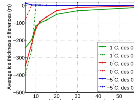
Figure 3. SG model vs. ISSM differences over an idealized
in-clined plane terrain. Average ice thickness differences (SG model −ISSM) are presented for simulations using different temperatures, desertification effect factors and number of hypsometric bins.
3.1.1 Inclined plane test
The bed topography for this test is an inclined plane topogra-phy with a constant slope of 0.014 and a maximum basal ele-vation of 800 m. For this case, the accuracy of the SG model correlates with the number of hypsometric bins as shown in Fig. 3 (ice and velocity profiles are shown in Fig. S1 in the Supplement). Reducing the number of SG bins increases the surface gradient between two hypsometric bins and thereby the computed ice velocities. With 10 hypsometric bins, the ice volume simulated by the SG model can be as low as 40 % of the ISSM prediction. The misfits are not significant in sim-ulations where no ablation is present (e.g. for a temperature set to−5◦C).
3.1.2 Rocky Mountains test
The SG model is tested on 21 regions from the Canadian Rockies, representing a wide range of topographic complex-ity (e.g. Fig. 4a), altitude (e.g. Fig. 4b) and slopes (e.g. Fig. 4c). The slopes of these regions are higher than in the inclined plane case. We focus on the results for simulations over the six test regions in Fig. 4 forced with sea level tem-perature of 0◦C and a desertification effect factor of 0.5. The results of other simulations, using different regions and with similar forcing as used in the inclined plane experiments, are not shown as they present similar misfits against ISSM re-sults.
complica-y coordinates (km)
region 1
20
40
60 1000
1500 2000
region 2
1000 1200 1400 1600 1800
region 3
800 1000 1200 1400
region 4
10 20 30 20
40
60 200
400 600
x coordinates (km) region 5
10 20 30
1000 1200 1400 1600 1800
region 6
10 20 30
1200 1400 1600 1800 2000
a.
0 1000 2000
region 1
Elevation (m)
region 2 region 3
0 0.5 1
0 1000 2000
region 4
0 0.5 1
region 5
Normalized cumulative subgrid area
0 0.5 1
region 6
b.
0 0.1
0.2 region 1
Slope
region 2 region 3
0 0.5 1
0 0.1
0.2 region 4
0 0.5 1
region 5
Normalized cumulative subgrid area
0 0.5 1
region 6
c.
Figure 4. Topography characteristics for six regions over the Canadian Rockies. (a) summarizes surface elevations, (b) the hypsometric
curves, and (c) the mean slope for each hypsometric bin.
tion for the “real” topography scenario comes from topo-graphic “jumps” not addressed in the SG model. Some high resolution adjacent grid cells belong to non-adjacent hypso-metric bins. The ice flow between these two locations is not accurately captured. The number of “jumps” increases with the number of bins used (Fig. S2 in the Supplement). A total of 10 hypsometric bins are then used to limit this effect. Even so, the SG model generates 45 % less to 15 % more ice than ISSM simulations (25 % less on average), depending on the regional topographic characteristics. No relation was found between the geographic complexity and the performance of the model, as explained in Sect. 3.2.
3.2 Test of alternative parameterizations
We examine the impact of including more topographic char-acteristics in the velocity parameterization. Charchar-acteristics considered include the flow direction, the terrain ruggedness (measured as the variation in three-dimensional orientation using a radius of 5 grid cells around the grid cell of interest), the sum of the squared slopes, the variance in the slopes, the number of local maxima (tested with radius sizes of 2, 6 and
10 grid cells) and the standard deviation of the surface eleva-tion topography.
5 10 15 20 25 30 0.5
0.6 0.7 0.8 0.9 1 1.1
Ice volume ratio
number of hypsometric levels
region1 region2 region3 region4 region5 region6
Figure 5. Ratio of the SG model over ISSM total ice volume for
six different regions in the Rockies as a function of hypsometric bins. The simulations were run until steady state with a constant sea level temperature of 0◦C and a desertification effect factor of 0.5. The steady state ice thicknesses, velocities and slopes from the ISSM and the SG model (using 10 hypsometric bins) are presented in Fig. S3 in the Supplement.
5 10 15 20
0 50 100 150 200 250 300 350
Region
Average ice thickness (m)
ISSM SG
regression model
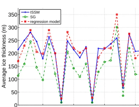
Figure 6. Average ice thickness in metres for different topographic
regions in the Rockies. Results are shown for the ISSM, the regres-sion model (generated by the stepwise regresregres-sion fit including only the standard deviation of the topography) and the SG model using 10 hypsometric bins.
Fig. 6) when the regression model generated using the stan-dard deviation of the topography is used. More details about the results of the stepwise regression fits are provided in the Supplement.
To explore potential improvement from accounting for the standard deviation of the high resolution topography,SSD, we
5 10 15 20
100 200 300 400 500
Ice thickness RMSE (m)
Region
No parametrization Para 1 Para 2
Figure 7. Average ice thickness root mean square error (RMSE)
between the ISSM and the SG model for different topographic re-gions. Simulations are run over 2 kyr using a constant precipitation rate of 1 m yr−1and a sea level temperature forcing of 0◦C. Dif-ferent SG parameterizations are presented. Para 1 is the standard deviation of the topography parameterization (Eq. 6) and Para 2 the lowest hypsometric slope parameterization (Eq. 7).
test the following parameterization of the velocity,u1:
u1= 2 5(ρg)
3A 0
P1H SSDP2
P3∂hd
∂x
3
. (6)
This equation is used in a simulation initialized with the ice thickness, velocities and slopes of ISSM values at steady state. The parametersP1,P2andP3(respectively 4.87, 0.016 and 2.8) are obtained using a least-squares approach that minimizes the differences between the velocities computed by ISSM and the SG model after one iteration (0.01-year).
The lowest hypsometric bin has the most significant mis-fits (e.g. Fig. S4 in the Supplement). This is likely related to the margin ice cliff slope parameterization. To try to correct this, we test the following parameterization for the lowest hypsometric bin velocity:
u2,N=
2 5(ρg)
3A 0HN4
P4HNP5 ∂hd,N
∂x
3
. (7)
Using the same least-squares approach as above, the pa-rameters P4 and P5 are respectively set to 5924.4 and −1.6383. These two parameterizations do not reduce the ice thickness differences with ISSM transient results (see Fig. 7). Ice thickness, velocities and slopes over the six re-gions analysed are presented for the different parameteriza-tions in Fig. S5 of the Supplement. As the model is highly non-linear, the improvement generated by the least-squares fit method for an initialization with ISSM steady state condi-tions does not persist over 1000-year runs.
0 1000 2000
Elevation (m)
region 1 region 2 region 3
0 0.5 1
0 1000 2000
region 4 5 levels 10 levels 10 levels flux issm bedrock
0 0.5 1
Cumulative normalized area
region 5
0 0.5 1
region 6
Figure 8. Surface elevation generated by the ISSM (solid blue line),
the SG model with no flux term, using 5 and 10 hypsometric bins, (dotted lines) and the SG model including the flux term (solid thin red line). These simulations use a constant sea level temperature of 0◦C and a desertification effect factor of 0.5. Results are shown at steady state after 2 kyr for six different regions with different topo-graphic characteristics.
The central difference discretization of the ice thickness in the effective diffusivity coefficient was replaced by an up-wind scheme. Simulations with different values of the Arrhe-nius coefficient, the power of the ice thickness and the slope, in Eq. (4), were analysed. An extra parameter was added in the velocity equation to account for neglected stresses. Turn-ing off the internal SG model flux term increased the misfits with ISSM simulations by a minimum of 100 % (as shown in Fig. 8). The basal elevation downstream of the terminus has been computed using a linear extrapolation of two or three upstream bins. The lowest hypsometric bin effective length generated with these basal elevations did not reduce the mis-fits with ISSM results.
4 Behaviour of the sub-grid model in the GSM
We present results of simulations over the last glacial cy-cle. The 39 “ensemble parameters” of the GSM (attempt-ing to capture the largest uncertainties in climate forc(attempt-ing, ice calving, and ice dynamics) have been subject to a Bayesian calibration against a large set of palaeoconstraints for the deglaciation of North America, as detailed in Tarasov et al. (2012). We use a high-scoring sub-ensemble of 600 param-eter vectors from this calibration to compare the GSM be-haviour when the SG model is turned on and off. The pri-mary supplement of Tarasov et al. (2012) includes a tabular description of the 39 ensemble parameters as well as input data sets. For the purposes of clarity and computational cost, we examined model sensitivity to different coupling and flux parameters using five parameter vectors (of the 600 members
2000 2500 3000 3500 4000 4500 5000 5500 6000
0 0.2 0.4 0.6 0.8 1
Elevation (m)
Normalized cumulative area hd 10 years hd 200 years hb hdhyps 10 years hdhyps 200 years hbhyps
a.
500 1000 1500 2000 2500 3000 3500
0 0.2 0.4 0.6 0.8 1
Elevation (m)
Normalize area
hd 10 years hd 200 years hb hdhyps 10 years hdhyps 200 years hbhyps
b.
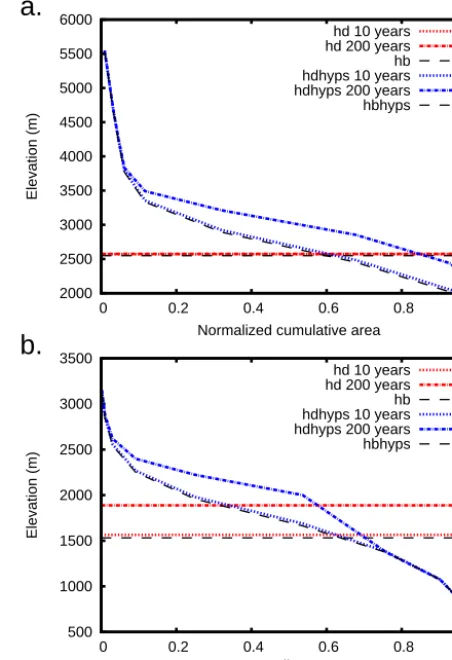
Figure 9. Elevation comparisons when the SG model is turned on
(blue) or off (red) at different time steps using the parameter vec-tor nn9894.hd10 years is the CG surface elevation after 10 years.
hdhyps10 years is the SG surface elevation.hbis the basal eleva-tion. (a) and (b) represent cases where the ELA is above and below the coarse grid surface elevation.
ensemble) that gave some of the best fits to the calibration constraints. As these five parameter vectors display similar behaviour, we present sensitivity results using the parameter vectors for the two runs described in detail in Tarasov et al. (2012) (identified in that paper as runs nn9894 and nn9927). For ease of interpretation, the ice volumes are presented as eustatic sea level (e.s.l.) equivalent3.
4.1 Last glacial cycle simulations over North America
The SG model can significantly alter the pattern of ice accu-mulation and loss. Figure 9 shows an example, for one of the parameter vectors of the ensemble of simulations, where SG ice accumulates while it melts at the CG level (Fig. 9a), and an example where CG ice is about 60 % greater than the SG ice (Fig. 9b).
-1 0 1 2 3 4 5 6
-120 -100 -80 -60 -40 -20 0
Eustatic sea level equivalent (m)
Time (ky) average (SG on - SG off)
standard deviation
Figure 10. Ensemble mean (solid red line) and standard deviation
(dotted blue line) eustatic sea level equivalent of the total ice volume differences when the SG model is turned on and off, for an ensemble run over the last glacial cycle.
The ensemble of simulations of the last glacial cycle over North America with the SG model activated generates, on average, between 0 and 1 m e.s.l.more ice than when the SG model is turned off (Fig. 10).
The impact of the SG model depends, however, on the cli-mate forcing and the ice sheet extent and elevations. During inception, when the SG model is turned on, ice accumulating in higher regions flows downhill and accumulates in regions close to the ELA and in valleys (Fig. 11). This allows, for ex-ample, ice to build up in the northern part of Alaska. For typ-ical runs, the ice generated by the SG model in the Alaskan Peninsula is, however, insufficient as compared to geological inferences (Dyke, 2004). The ensemble mean and standard deviation of the differences between runs with SG on and off at 110 ka, are respectively 0.4 and 1 m e.s.l.However, at spe-cific time slices, the differences can be much larger. Once the ice sheet has grown to a sizeable fraction of LGM extent, for example at 50 ka, the standard deviation of the ensemble-run differences (between SG on and off) reaches 5 m e.s.l. Fig-ure 12 shows an example where ice in a region of low altitude in the centre of Canada is not allowed to grow when the SG model is used. On the other hand, a simulation using different ensemble parameters generates ice in this region only when the SG model is turned on (Fig. S6 in the Supplement). In extreme cases, differences can reach tens of m e.s.l.(Fig. S7 in the Supplement). We could not identify a reason for the strong sensitivity of ice volume around 50 ka other than the inherent non-linearity of the GSM.
4.2 Sensitivity of the model to different flux and coupling parameters
The accounting of SG fluxes has varying impacts over a glacial cycle simulation (Fig. 13). At 50 ka, for example, the total ice volume with parameter vector nn9894 is reduced by
a.
b.
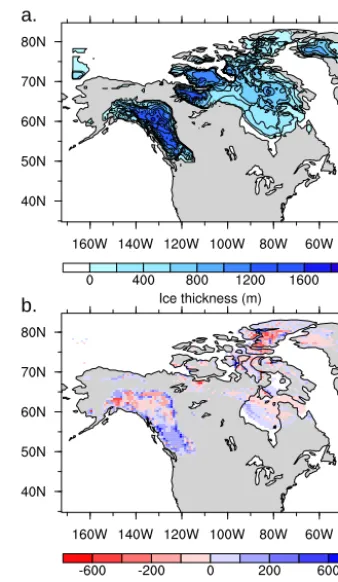
Figure 11. Ice field during inception at 115 ka for a simulation using
one of the parameter vectors that generates best fits to the calibra-tion constraints (nn9894). (a) Ice thickness with SG turned on. (b) Ice thickness differences between simulations with the SG model turned on and off. Zero differences are presented in the same colour as the continent.
50 % when SG fluxes are included. During inception, on the other hand, inclusion of SG fluxes increases the total amount of CG ice (Fig. 14, again with nn9894).
al-a.
b.
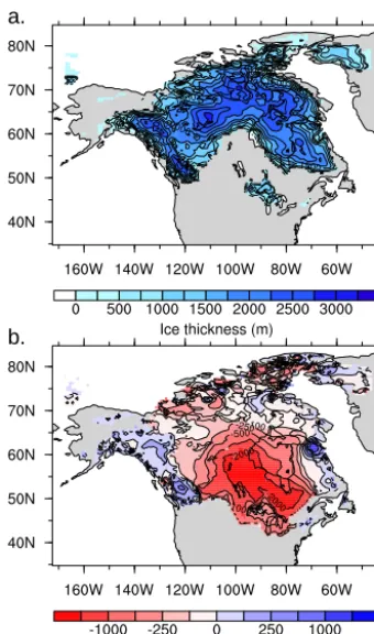
Figure 12. Ice field at 50 ka for a simulation using parameter
nn9894. (a) Ice thickness with SG turned on. (b) Ice thickness dif-ferences between simulations with the SG model turned on and off.
lowing ice fluxes out of coarse grid cells with SG activated generates higher or lower ice volumes (Fig. 13). Moreover, 50 ka is an example of a 60 % increase of the total ice volume when the fluxes out of coarse grid cells (with SG activated) are not allowed. As a counter-example, 35 ka presents a case where turning off the fluxes out of (SG activated) coarse grid cells decreases the total ice volume.
With Marshall et al.’s (2011) flux equation, differences be-tween runs with SG fluxes turned on versus off are negligible over the full glacial cycle (Fig. 14).
As described in Sect. 2.3.1, the CG ice thickness used by the GSM conserves the ice volume of the filled SG bins (vol-ume conservation, VC, method). As this ice is redistributed over the total area of the coarse grid cell, the surface eleva-tion of the ice, and consequently the fluxes, are underesti-mated. The surface gradient between adjacent cells is then lower than the gradient at the SG level. We tested setting the CG surface elevation to the maximum value between the sur-face elevation of the coarse grid cell and the lowest hypso-metric bin (surface conservation (SC) method). We also im-plemented a method using the maximum surface elevation generated by the two former methods (maximum conserva-tion (MC) method). During incepconserva-tion (between 118 and 114 ka) the VC method generates between 10 and 20 % (which is equivalent to 0.5–1 m e.s.l.) more ice than the two other
0 10 20 30 40 50 60 70 80 90
-120 -100 -80 -60 -40 -20 0
Eustatic sea level equivalent (m)
Time (ky) SG OFF
flux on flux off NofluxOut
Figure 13. Total ice volume evolution for a simulation using
pa-rameter vector nn9894. “flux on” and “flux off” both include the SG surface mass balance calculations but the latter has no SG ice fluxes. “NofluxOut” has SG on, but no SG ice flux between coarse grid cells. The “SG OFF” line is most of the time hidden under the “flux off” line.
0 2 4 6 8 10 12
-120 -119 -118 -117 -116 -115 -114
Eustatic sea level equivalent (m)
Time (ky) our flux Marshall flux flux off our flux NofluxOut
Figure 14. Ice volume evolution for a simulation over North
Amer-ica (parameter vector nn9894) with the SG model turned on during inception. “our flux” represents the flux code used in our SG model and “Marshall flux” the flux code used in Marshall et al. (2011) experiment. “flux off” represents the simulation with no ice flux be-tween SG bins and “NofluxOut” has no SG flux bebe-tween coarse grid cells (but SG fluxes within each coarse grid cell are still enabled).
0 1 2 3 4 5 6 7 8 9 10
-120 -119 -118 -117 -116 -115 -114
Eustatic sea level equivalent (m)
Time (ky) SG off
SG on, VC SG on, SC SG on, MC
Figure 15. Total ice volume evolution for a simulation over North
America during inception with the SG model turned on (SG on) using the parameter vector of run nn9927. Different methods of ice redistribution at the CG level are compared. VC is for ice volume conservation, SC for surface elevation conservation and MC uses the maximum of the previous two methods. “SG off” represents a run where the SG model has been turned off.
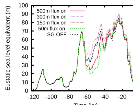
Figure 16 shows the results of the glacial cycle simulation when the SG model is turned off and when the minimum al-titude variation SG activation threshold is set to 50, 150, 300 and 500 m. A non-linear dependence on the threshold can be observed. At 50 ka, for example, setting the threshold to 50 m generates the lowest total ice volume while a thresh-old of 150 m leads to the highest ice volume. The difference between these two runs is 34.5 m e.s.l.at 50 ka. Thresholds of 300 and 500 m generate intermediate total ice volumes. Moreover, simulations using different parameter vectors (not shown) result in different behaviours. No conclusion could be drawn about the optimal threshold.
5 Conclusions
Our new sub-grid surface mass balance and flux model ex-tends the initial work of Marshall and Clarke (1999) and Marshall et al. (2011). The evaluation of the model, done for the first time against results from a high resolution higher order model (ISSM), demonstrates that
– Depending on the regional topographic characteristics, the new SG model simulates ice volumes 45 % lower to 15 % higher than simulated by the ISSM (using 10 hyp-sometric bins). Increasing the number of hyphyp-sometric bins to more than 10 did not reduce misfits for simula-tions over rough topographic regions extracted from the Canadian Rockies.
– Turning off the SG internal fluxes increases the ice vol-ume misfits with ISSM simulations by a minimum of 100 %.
0 10 20 30 40 50 60 70 80 90 100
-120 -100 -80 -60 -40 -20 0
Eustatic sea level equivalent (m)
Time (ky) 500m flux on
300m flux on 150m flux on 50m flux on SG OFF
Figure 16. Total ice volume evolution for a simulation using
pa-rameter vector nn9894. Different curves represent simulations with different minimum altitude variation thresholds used for the SG ac-tivation.
– Increasing the number of topography characteristics used in the SG model, as suggested by Marshall and Clarke (1999), did not reduce the misfits with the high resolution model during transient runs.
An ensemble of simulations over the last glacial cycle of the North American ice complex shows, on average, an in-crease of ice generated with inclusion of the SG model. The ensemble mean for each time step is between 0 and 1 m e.s.l., with a standard deviation of a minimum of twice the mean and reaching 5 m e.s.l.at 50 ka). At the end of inception, at 110 ka, the increase of ice volume from SG model inclu-sion is still insufficient over the Alaska Peninsula when com-pared to geological inferences. Over the glacial cycle, the SG model generates different patterns of ice extent. In some in-stances, the SG model prevents ice growth, while in others it enables extra ice build up over thousands of square kilome-tres.
Simulated ice evolution is sensitive to the treatment of ice fluxes within the SG model and between the SG and CG lev-els.
– The flux term has an important impact on the SG model. Not allowing ice to flow between hypsometric bins in-creases the total ice volume with a maximum increase of 50 % at 50 ka (in a glacial cycle run). During incep-tion, however, the flux module can generate more ice. Different parameterizations of the flux term impact the results. A SG ice rheology parameter corresponding to ice at about−40◦C (as used in Marshall et al., 2011) generates the same amount of ice during inception as when the flux term is off.
about −40◦C, generates an ice volume higher than
when a flux parameterization with a rheology value rep-resenting ice at about 0◦C is used.
– Not allowing ice to flow out of a CG cell where SG is activated increases or decreases the total ice volume depending of the ice configuration. At 50 ka, the total increases by 60 %.
– The ice configuration from simulations over the last glacial cycle of North America is sensitive to the choice of SG to CG ice redistribution scheme.
We have identified the representation of SG fluxes between CG cells to be a challenging issue that can significantly im-pact modelling ice sheet evolution.
We have shown that the above geometric and ice dynam-ics factors can have significant impacts on modelled ice sheet evolution (with up to a 35 m e.s.l.difference in North Amican ice volume at 50 ka). Therefore, signifAmicant potential er-rors may arise if sub-grid mass-balance and fluxes are not accounted for in the coarse resolutions required for glacial cycle ice sheet models. Other alternatives to the hypsomet-ric parameterization, such as running a high resolution SIA model in the region of rough topography, could be consid-ered. One issue we have not examined is the downscaling of the climatic forcing. Temperature and especially precipita-tion can exhibit strong vertical gradients in mountainous re-gions. Whether this can have significant impact on CG scales is unclear. Improvements of the precipitation representation are possible using, for instance, a linear model of orographic precipitation for downscaling climatic inputs (Jarosch et al., 2012).
Code availability
The sub-grid code is available upon request from the first two authors.
The Supplement related to this article is available online at doi:10.5194/gmd-8-3199-2015-supplement.
Author contributions. Kevin Le Morzadec and Lev Tarasov de-signed the experiments. Kevin Le Morzadec developed the SG model code and performed the simulations. Kevin Le Morzadec and Lev Tarasov coupled the SG model into the GSM. Mathieu Morlighem and Helene Seroussi supported ISSM installation and helped build a new surface mass balance module for the ISSM. Kevin Le Morzadec prepared the manuscript with contributions from Lev Tarasov and the other co-authors. Lev Tarasov heavily edited the manuscript.
Acknowledgements. We thank Vincent Lecours and Rodolphe Devillers for extracting some of the topographic characteristics. Support provided by the Canadian Foundation for Innovation, the National Science and Engineering Research Council, and ACEnet. Tarasov holds a Canada Research Chair. We finally thank Philippe Huybrechts, as well as Fuyuki Saito and an anonymous reviewer, whose comments helped significantly improve the clarity of the manuscript.
Edited by: D. Roche
References
Abe-Ouchi, A. and Blatter, H.: On the initiation of ice sheets, Ann. Glaciol., 18, 203–203, 1993.
Abe-Ouchi, A., Saito, F., Kawamura, K., Raymo, M. E., Okuno, J., Takahashi, K., and Blatter, H.: Insolation-driven 100,000-year glacial cycles and hysteresis of ice-sheet volume, Nature, 500, 190–193, 2013.
BODC: British oceanographic data centre, The GEBCO_08 Grid, version 20091120, available at: http://www.gebco.net (last ac-cess: 6 October 2013), 2010.
Budd, W. F. and Smith, I.: The growth and retreat of ice sheets in re-sponse to orbital radiation changes, Sea Level, Ice, and Climatic Change, 369–409, 1981.
Clarke, G. K.: Fast glacier flow: ice streams, surging, and tidewater glaciers, J. Geophys. Res.-Sol. Ea., 92, 8835–8841, 1987. Colleoni, F., Masina, S., Cherchi, A., Navarra, A., Ritz, C., Peyaud,
V., and Otto-Bliesner, B.: Modeling Northern Hemisphere ice-sheet distribution during MIS 5 and MIS 7 glacial inceptions, Clim. Past, 10, 269–291, doi:10.5194/cp-10-269-2014, 2014. Dansgaard, W., Johnsen, S., Clausen, H., Dahl-Jensen, D.,
Gunde-strup, N., Hammer, C., Hvidberg, C., Steffensen, J., Sveinbjörns-dottir, A., Jouzel, J., and Bond, G.: Evidence for general instabil-ity of past climate from a 250-kyr ice-core record, Nature, 364, 218–220, 1993.
Durand, G., Gagliardini, O., Favier, L., Zwinger, T., and Le Meur, E.: Impact of bedrock description on model-ing ice sheet dynamics, Geophys. Res. Lett., 38, L20501, doi:10.1029/2011GL048892, 2011.
Dyke, A. S.: An outline of North American deglaciation with em-phasis on central and northern Canada, Quaternary glaciations – Extent and chronology, 2, 373–424, 2004.
Franco, B., Fettweis, X., Lang, C., and Erpicum, M.: Impact of spa-tial resolution on the modelling of the Greenland ice sheet sur-face mass balance between 1990–2010, using the regional cli-mate model MAR, The Cryosphere, 6, 695-711, doi:10.5194/tc-6-695-2012, 2012.
Fulton, R.: Surficial Materials Map of Canada, 1995.
Gardner, A. S., Sharp, M. J., Koerner, R. M., Labine, C., Boon, S., Marshall, S. J., Burgess, D. O., and Lewis, D.: Near-surface tem-perature lapse rates over Arctic glaciers and their implications for temperature downscaling, J. Climate, 22, 4281–4298, 2009. Giorgi, F., Francisco, R., and Pal, J.: Effects of a subgrid-scale
Jarosch, A. H., Anslow, F. S., and Clarke, G. K.: High-resolution precipitation and temperature downscaling for glacier models, Clim. Dynam., 38, 391–409, 2012.
Josenhans, H. and Zevenhuizen, J.: Dynamics of the Laurentide ice sheet in Hudson Bay, Canada, Mar. Geol., 92, 1–26, 1990. Kalnay, E., Kanamitsu, M., Kistler, R., Collins, W., Deaven, D.,
Gandin, L., Iredell, M., Saha, S., White, G., Woollen, J., Zhu, Y., Leetmaa, A., Reynolds, R., Chelliah, M., Ebisuzaki, W. abd Hig-gins, W., Janowiak, J., Mo, K. C., Ropelewski, C., Wang, J., Jenne, R., and Joseph, D.: The NCEP/NCAR 40-year reanalysis project, Bull. Am. Meteorol. Soc., 77, 437–471, 1996.
Ke, Y., Leung, L. R., Huang, M., and Li, H.: Enhancing the repre-sentation of subgrid land surface characteristics in land surface models, Geosci. Model Dev., 6, 1609–1622, doi:10.5194/gmd-6-1609-2013, 2013.
Larour, E., Seroussi, H., Morlighem, M., and Rignot, E.: Continen-tal scale, high order, high spatial resolution, ice sheet modeling using the Ice Sheet System Model (ISSM), J. Geophys. Res., 117, F01022, doi:10.1029/2011JF002140, 2012.
Laske, G. and Masters, G.: A global digital map of sediment thick-ness, Eos Trans. AGU, 78, F483, 1997.
Leung, L. R. and Ghan, S.: A subgrid parameterization of oro-graphic precipitation, Theor. Appl. Climatol., 52, 95–118, 1995. Marshall, S.: Modelled nucleation centres of the Pleistocene ice sheets from an ice sheet model with subgrid topographic and glaciologic parameterizations, Quaternary Int., 95, 125–137, 2002.
Marshall, S. and Clarke, G.: Ice sheet inception: subgrid hypsomet-ric parameterization of mass balance in an ice sheet model, Clim. Dynam., 15, 533–550, 1999.
Marshall, S. J. and Losic, M.: Temperature lapse rates in glacier-ized basins, in: Encyclopedia of Snow, Ice and Glaciers, Springer,1145–1150, 2011.
Marshall, S. J., White, E. C., Demuth, M. N., Bolch, T., Wheate, R., Menounos, B., Beedle, M. J., and Shea, J. M.: Glacier water re-sources on the eastern slopes of the Canadian Rocky Mountains, Can. Water Resour. J., 36, 109–134, 2011.
Payne, A. and Sugden, D.: Topography and ice sheet growth, Earth Surf. Proc. Landf., 15, 625–639, 1990.
Payne, A., Huybrechts, P., Abe-Ouchi, A., Calov, R., Fastook, J., Greve, R., Marshall, S., Marsiat, I., Ritz, C., Tarasov, L., and Thomassen, M. P. A.: Results from the EISMINT model intercomparison: the effects of thermomechanical coupling, J. Glaciol., 46, 227–238, 2000.
Pollard, D. and DeConto, R. M.: Description of a hybrid ice sheet-shelf model, and application to Antarctica, Geosci. Model Dev., 5, 1273–1295, doi:10.5194/gmd-5-1273-2012, 2012.
Seth, A., Giorgi, F., and Dickinson, R. E.: Simulating fluxes from heterogeneous land surfaces: explicit subgrid method employing the biosphere-atmosphere transfer scheme (BATS), J. Geophys. Res., 99, 18651–18667, 1994.
Tangborn, W.: Mass balance, runoff and surges of Bering Glacier, Alaska, The Cryosphere, 7, 867–875, doi:10.5194/tc-7-867-2013, 2013.
Tarasov, L. and Peltier, W.: Impact of thermomechanical ice sheet coupling on a model of the 100 kyr ice age cycle, J. Geophys. Res.-Atmos., 104, 9517–9545, 1999.
Tarasov, L. and Peltier, W.: Greenland glacial history and local geo-dynamic consequences, Geophys. J. Int., 150, 198–229, 2002. Tarasov, L. and Peltier, W.: A geophysically constrained large
en-semble analysis of the deglacial history of the North American ice-sheet complex, Quaternary Sci. Rev., 23, 359–388, 2004. Tarasov, L. and Peltier, W.: Arctic freshwater forcing of the Younger
Dryas cold reversal, Nature, 435, 662–665, 2005.
Tarasov, L. and Peltier, W.: A calibrated deglacial drainage chronol-ogy for the North American continent: evidence of an Arctic trig-ger for the Yountrig-ger Dryas, Quaternary Sci. Rev., 25, 659–688, 2006.
Tarasov, L. and Peltier, W.: Coevolution of continental ice cover and permafrost extent over the last glacial-interglacial cycle in North America, J. Geophys. Res., 112, F02S08, doi:10.1029/2006JF000661, 2007.
Tarasov, L. and Peltier, W. R.: Terminating the 100 kyr Ice Age cycle, J. Geophys. Res., 102, 21665–21693, 1997.
Tarasov, L., Dyke, A. S., Neal, R. M., and Peltier, W.: A data-calibrated distribution of deglacial chronologies for the North American ice complex from glaciological modeling, Earth Planet. Sci. Lett., 315, 30–40, 2012.
Van den Berg, J., Van de Wal, R., and Oerlemans, J.: Effects of spatial discretization in ice-sheet modelling using the shallow-ice approximation, J. Glaciol., 52, 89–98, 2006.