www.geosci-model-dev.net/9/1937/2016/ doi:10.5194/gmd-9-1937-2016
© Author(s) 2016. CC Attribution 3.0 License.
Overview of the Coupled Model Intercomparison Project Phase 6
(CMIP6) experimental design and organization
Veronika Eyring1, Sandrine Bony2, Gerald A. Meehl3, Catherine A. Senior4, Bjorn Stevens5, Ronald J. Stouffer6, and Karl E. Taylor7
1Deutsches Zentrum für Luft- und Raumfahrt (DLR), Institut für Physik der Atmosphäre, Oberpfaffenhofen, Germany 2Laboratoire de Météorologie Dynamique, Institut Pierre Simon Laplace (LMD/IPSL), CNRS,
Université Pierre et Marie Curie, Paris, France
3National Center for Atmospheric Research (NCAR), Boulder, CO, USA 4Met Office Hadley Centre, Exeter, UK
5Max-Planck-Institute for Meteorology, Hamburg, Germany
6Geophysical Fluid Dynamics Laboratory/NOAA, Princeton, NJ, USA 7Program for Climate Model Diagnosis and Intercomparison (PCMDI),
Lawrence Livermore National Laboratory, Livermore, CA, USA Correspondence to:Veronika Eyring ([email protected])
Received: 3 December 2015 – Published in Geosci. Model Dev. Discuss.: 14 December 2015 Revised: 15 April 2016 – Accepted: 27 April 2016 – Published: 26 May 2016
Abstract. By coordinating the design and distribution of global climate model simulations of the past, current, and future climate, the Coupled Model Intercomparison Project (CMIP) has become one of the foundational elements of climate science. However, the need to address an ever-expanding range of scientific questions arising from more and more research communities has made it necessary to re-vise the organization of CMIP. After a long and wide com-munity consultation, a new and more federated structure has been put in place. It consists of three major elements: (1) a handful of common experiments, the DECK (Diagnostic, Evaluation and Characterization of Klima) and CMIP his-torical simulations (1850–near present) that will maintain continuity and help document basic characteristics of mod-els across different phases of CMIP; (2) common standards, coordination, infrastructure, and documentation that will fa-cilitate the distribution of model outputs and the characteriza-tion of the model ensemble; and (3) an ensemble of CMIP-Endorsed Model Intercomparison Projects (MIPs) that will be specific to a particular phase of CMIP (now CMIP6) and that will build on the DECK and CMIP historical simulations to address a large range of specific questions and fill the sci-entific gaps of the previous CMIP phases. The DECK and CMIP historical simulations, together with the use of CMIP
data standards, will be the entry cards for models participat-ing in CMIP. Participation in CMIP6-Endorsed MIPs by in-dividual modelling groups will be at their own discretion and will depend on their scientific interests and priorities. With the Grand Science Challenges of the World Climate Research Programme (WCRP) as its scientific backdrop, CMIP6 will address three broad questions:
– How does the Earth system respond to forcing? – What are the origins and consequences of systematic
model biases?
– How can we assess future climate changes given inter-nal climate variability, predictability, and uncertainties in scenarios?
1 Introduction
The Coupled Model Intercomparison Project (CMIP) orga-nized under the auspices of the World Climate Research Pro-gramme’s (WCRP) Working Group on Coupled Modelling (WGCM) started 20 years ago as a comparison of a handful of early global coupled climate models performing experi-ments using atmosphere models coupled to a dynamic ocean, a simple land surface, and thermodynamic sea ice (Meehl et al., 1997). It has since evolved over five phases into a ma-jor international multi-model research activity (Meehl et al., 2000, 2007; Taylor et al., 2012) that has not only introduced a new era to climate science research but has also become a central element of national and international assessments of climate change (e.g. IPCC, 2013). An important part of CMIP is to make the multi-model output publicly available in a standardized format for analysis by the wider climate com-munity and users. The standardization of the model output in a specified format, and the collection, archival, and access of the model output through the Earth System Grid Federation (ESGF) data replication centres have facilitated multi-model analyses.
The objective of CMIP is to better understand past, present, and future climate change arising from natural, un-forced variability or in response to changes in radiative forc-ings in a multi-model context. Its increasing importance and scope is a tremendous success story, but this very success poses challenges for all involved. Coordination of the project has become more complex as CMIP includes more models with more processes all applied to a wider range of ques-tions. To meet this new interest and to address a wide vari-ety of science questions from more and more scientific re-search communities, reflecting the expanding scope of com-prehensive modelling in climate science, has put pressure on CMIP to become larger and more extensive. Consequently, there has been an explosion in the diversity and volume of requested CMIP output from an increasing number of ex-periments causing challenges for CMIP’s technical infras-tructure (Williams et al., 2015). Cultural and organizational challenges also arise from the tension between expectations that modelling centres deliver multiple model experiments to CMIP yet at the same time advance basic research in climate science.
In response to these challenges, we have adopted a more federated structure for the sixth phase of CMIP (i.e. CMIP6) and subsequent phases. Whereas past phases of CMIP were usually described through a single overview paper, reflect-ing a centralized and relatively compact CMIP structure, this GMD special issue describes the new design and organiza-tion of CMIP, the suite of experiments, and its forcings, in a series of invited contributions. In this paper, we provide the overview and backdrop of the new CMIP structure as well as the main scientific foci that CMIP6 will address. We begin by describing the new organizational form for CMIP and the pressures that it was designed to alleviate (Sect. 2). It also
contains a description of a small set of simulations for CMIP which are intended to be common to all participating mod-els (Sect. 3), details of which are provided in the Appendix. We then present a brief overview of CMIP6 that serves as an introduction to the other contributions to this special issue (Sect. 4), and we close with a summary.
2 CMIP design – a more continuous and distributed organization
In preparing for CMIP6, the CMIP Panel (the authors of this paper), which traditionally has the responsibility for direct coordination and oversight of CMIP, initiated a 2-year pro-cess of community consultation. This consultation involved the modelling centres whose contributions form the sub-stance of CMIP as well as communities that rely on CMIP model output for their work. Special meetings were orga-nized to reflect on the successes of CMIP5 as well as the sci-entific gaps that remain or have since emerged. The consulta-tion also sought input through a community survey, the scien-tific results of which are described by Stouffer et al. (2015). Four main issues related to the overall structure of CMIP were identified.
First, we identified a growing appreciation of the scientific potential to use results across different CMIP phases. Such approaches, however, require an appropriate experimental design to facilitate the identification of an ensemble of mod-els with particular properties drawn from different phases of CMIP (e.g. Rauser et al., 2014). At the same time, it was recognized that an increasing number of Model Intercompar-ison Projects (MIPs) were being organized independent of CMIP, the data structure and output requirements were often inconsistent, and the relationship between the models used in the various MIPs was often difficult to determine, in which context measures to help establish continuity across MIPs or phases of CMIP would also be welcome.
Second, the scope of CMIP was taxing the resources of modelling centres making it impossible for many to consider contributing to all the proposed experiments. By providing a better basis to help modelling centres decide exactly which subset of experiments to perform, it was thought that it might be possible to minimize fragmented participation in CMIP6. A more federated experimental protocol could also encour-age modelling centres to develop intercomparison studies based on their own strategic goals.
Third, some centres expressed the view that the punctu-ated structure of CMIP had begun to distort the model devel-opment process. Defining a protocol that allowed modelling centres to decouple their model development from the CMIP schedule would offer additional flexibility, and perhaps en-courage modelling centres to finalize their models and sub-mit some of their results sooner on their own schedule.
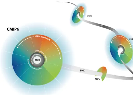
Figure 1.CMIP evolution. CMIP will evolve but the DECK will provide continuity across phases.
MIPs, but rather to reflect the strategic goals of the climate science community as, for instance, articulated by WCRP. By focusing a particular phase of CMIP around specific sci-entific issues, it was felt that the modelling resources could be more effectively applied to those scientific questions that had matured to a point where coordinated activities were ex-pected to have substantial impact.
A variety of mechanisms were proposed and intensely de-bated to address these issues. The outcome of these discus-sions is embodied in the new CMIP structure, which has three major components. First, the identification of a handful of common experiments, the Diagnostic, Evaluation and Char-acterization of Klima (DECK) experiments (klimais Greek for “climate”), and CMIP historical simulations, which can be used to establish model characteristics and serves as its en-try card for participating in one of CMIP’s phases or in other MIPs organized between CMIP phases, as depicted in Fig. 1. Second, common standards, coordination, infrastructure, and documentation that facilitate the distribution of model out-puts and the characterization of the model ensemble, and third, the adoption of a more federated structure, building on more autonomous CMIP-Endorsed MIPs.
Realizing the idea of a particular phase of CMIP being centred on a collection of more autonomous MIPs required
mod-Table 1.Main criteria for MIP endorsement as agreed with representatives from the modelling groups and MIPs at the WGCM 18th Session in Grainau, Germany in October 2014.
No. MIP endorsement criterion
1 The MIP and its experiments address at least one of the key science questions of CMIP6.
2 The MIP demonstrates connectivity to the DECK experiments and the CMIP6 historical simulations. 3 The MIP adopts the CMIP modelling infrastructure standards and conventions.
4 All experiments are tiered, well defined, and useful in a multi-model context and do not overlap with other CMIP6 experiments.
5 Unless a Tier 1 experiment differs only slightly from another well-established experiment, it must already have been performed by more than one modelling group.
6 A sufficient number of modelling centres (∼8) are committed to performing all of the MIP’s Tier 1 experiments and providing all the requested diagnostics needed to answer at least one of its science questions.
7 The MIP presents an analysis plan describing how it will use all proposed experiments, any relevant observa-tions, and specially requested model output to evaluate the models and address its science questions.
8 The MIP has completed the MIP template questionnaire.
9 The MIP contributes a paper on its experimental design to the GMD CMIP6 special issue. 10 The MIP considers reporting on the results by co-authoring a paper with the modelling groups.
elling groups indicated their intent to participate in Tier 1 ex-periments at least, thus attesting to the wide appeal and level of science interest from the climate modelling community.
3 The DECK and CMIP historical simulations
The DECK comprises four baseline experiments: (a) a his-torical Atmospheric Model Intercomparison Project (amip) simulation, (b) a pre-industrial control simulation (piCon-troloresm-piControl), (c) a simulation forced by an abrupt quadrupling of CO2 (abrupt-4×CO2) and (d) a simulation
forced by a 1 % yr−1 CO2 increase (1pctCO2). CMIP also
includes a historical simulation (historicalor esm-hist) that spans the period of extensive instrumental temperature mea-surements from 1850 to the present. In naming the experi-ments, we distinguish between simulations with CO2
con-centrations calculated and anthropogenic sources of CO2
prescribed (esm-piControl and esm-hist) and simulations with prescribed CO2 concentrations (all others). Hereafter,
models that can calculate atmospheric CO2 concentration
and account for the fluxes of CO2between the atmosphere,
the ocean, and biosphere are referred to as Earth System Models (ESMs).
The DECK experiments are chosen (1) to provide conti-nuity across past and future phases of CMIP, (2) to evolve as little as possible over time, (3) to be well established, and incorporate simulations that modelling centres perform any-way as part of their own development cycle, and (4) to be rel-atively independent of the forcings and scientific objectives of a specific phase of CMIP. The four DECK experiments and the CMIP historical simulations are well suited for quan-tifying and understanding important climate change response characteristics. Modelling groups also commonly perform simulations of the historical period, but reconstructions of the external conditions imposed on historical runs (e.g.
land-use changes) continue to evolve significantly, influencing the simulated climate. In order to distinguish among the histor-ical simulations performed under different phases of CMIP, the historical simulations are labelled with the phase (e.g. “CMIP5historical” or “CMIP6 historical”). A similar ar-gument could be made to exclude the AMIP experiments from the DECK. However, the AMIP experiments are sim-pler, more routine, and the dominating role of sea surface temperatures and the focus on recent decades means that for most purposes AMIP experiments from different phases of CMIP are more likely to provide the desired continuity.
The persistence and consistency of the DECK will make it possible to track changes in performance and response characteristics over future generations of models and CMIP phases. Although the set of DECK experiments is not ex-pected to evolve much, additional experiments may become enough well established as benchmarks (routinely run by modelling groups as they develop new model versions) so that in the future they might be migrated into the DECK. The common practice of including the DECK in model de-velopment efforts means that models can contribute to CMIP without carrying out additional computationally burdensome experiments. All of the DECK and the historical simulations were included in the core set of experiments performed under CMIP5 (Taylor et al., 2012), and all but theabrupt-4×CO2 simulation were included in even earlier CMIP phases.
different realizations. This would include, for example, a change in model resolution, physical processes, or atmo-spheric chemistry treatment. If an ESM is used in both CO2
-emission-driven mode and CO2-concentration-driven mode
in subsequent CMIP6-Endorsed MIPs, then both emission-driven and concentration-emission-driven control, and historical simu-lations should be done and they will be identical in all forc-ings except the treatment of CO2.
The forcing data sets that will drive the DECK and CMIP6 historical simulations are described separately in a series of invited contributions to this special issue. These articles also include some discussion of uncertainty in the data sets. The data will be provided by the respective author teams and made publicly available through the ESGF using common metadata and formats.
The historical forcings are based as far as possible on ob-servations and cover the period 1850–2014. These include:
– emissions of short-lived species and long-lived green-house gases (GHGs),
– GHG concentrations,
– global gridded land-use forcing data sets, – solar forcing,
– stratospheric aerosol data set (volcanoes),
– AMIP sea surface temperatures (SSTs) and sea ice con-centrations (SICs),
– for simulations with prescribed aerosols, a new ap-proach to prescribe aerosols in terms of optical prop-erties and fractional change in cloud droplet effective radius to provide a more consistent representation of aerosol forcing, and
– for models without ozone chemistry, time-varying grid-ded ozone concentrations and nitrogen deposition. Some models might require additional forcing data sets (e.g. black carbon on snow or anthropogenic dust). Allowing model groups to use different forcing1data sets might better sample uncertainty, but makes it more difficult to assess the uncertainty in the response of models to the best estimate of the forcing, available to a particular CMIP phase. To avoid conflating uncertainty in the response of models to a given forcing, it is strongly preferred for models to be integrated with the same forcing in the entry card historical simulations, and for forcing uncertainty to be sampled in supplementary
1Here, we distinguish between an applied input perturbation
(e.g. the imposed change in some model constituent, property, or boundary condition), which we refer to somewhat generically as a “forcing”, and radiative forcing, which can be precisely defined. Even if the forcings are identical, the resulting radiative forcing de-pends on a model’s radiation scheme (among other factors) and will differ among models.
simulations that are proposed as part of DAMIP. In any case it is important that all forcing data sets are documented and are made available alongside the model output on the ESGF. Likewise to the extent modelling centres simplify forcings, for instance by regridding or smoothing in time or some other dimension, this should also be documented.
For the future scenarios selected by ScenarioMIP, forcings are provided by the integrated assessment model (IAM) com-munity for the period 2015–2100 (or until 2300 for the ex-tended simulations). For atmospheric emissions and concen-trations as well as for land use, the forcings are harmonized across IAMs and scenarios using a similar procedure as in CMIP5 (van Vuuren et al., 2011). This procedure ensures consistency with historical forcing data sets and between the different forcing categories. The selection of scenarios and the main characteristics are described elsewhere in this spe-cial issue, while the underlying IAM scenarios are described in a special issue in Global Environmental Change.
An important gap identified in CMIP5, and in previous CMIP phases, was a lack of careful quantification of the ra-diative forcings from the different specified external forcing factors (e.g. GHGs, sulphate aerosols) in each model (Stouf-fer et al., 2015). This has impaired attempts to identify rea-sons for differences in model responses. The effective ra-diative forcing or ERF component of the Rara-diative Forcing MIP (RFMIP) includes fixed SST simulations to diagnose the forcing (RFMIP-lite), which are further detailed in the corresponding contribution to this special issue. Although not included as part of the DECK, in recognition of this de-ficiency in past phases of CMIP we strongly encourage all CMIP6 modelling groups to participate in RFMIP-lite. The modest additional effort would enable the radiative forcing to be characterized for both historic and future scenarios across the model ensemble. Knowing this forcing would lead to a step change in efforts to understand the spread of model re-sponses for CMIP6 and contribute greatly to answering one of CMIP6’s science questions.
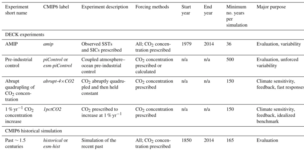
An overview of the main characteristics of the DECK and CMIP6 historical simulations appears in Table 2. Here we briefly describe these experiments. Detailed specifications for the DECK and CMIP6 historical simulations are provided in Appendix A and are summarized in Table A1.
3.1 The DECK
The AMIP and pre-industrial control simulations of the DECK provide opportunities for evaluating the atmospheric model and the coupled system, and in addition they establish a baseline for performing many of the CMIP6 experiments. Many experiments branch from, and are compared with, the pre-industrial control. Similarly, a number of diagnostic at-mospheric experiments use AMIP as a control. The idealized CO2-forced experiments in the DECK (abrupt-4×CO2 and
Table 2.Overview of DECK and CMIP6 historical simulations providing the experiment short names, the CMIP6 labels, brief experiment descriptions, the forcing methods, as well as the start and end year and minimum number of years per experiment and its major purpose. The DECK and CMIP6 historical simulation are used to characterize the CMIP model ensemble. Given resource limitations, these entry card simulations for CMIP include only one ensemble member per experiment. However, we strongly encourage model groups to submit at least three ensemble members for the CMIP historical simulation as requested in DAMIP. Large ensembles of AMIP simulations are also encouraged. In the “forcing methods” column, “All” means “volcanic, solar, and anthropogenic forcings”. All experiments are started on 1 January and end on 31 December of the specified years.
Experiment short name
CMIP6 label Experiment description Forcing methods Start year
End year
Minimum no. years per simulation
Major purpose
DECK experiments
AMIP amip Observed SSTs
and SICs prescribed
All; CO2 concen-tration prescribed
1979 2014 36 Evaluation, variability
Pre-industrial control
piControlor
esm-piControl
Coupled atmosphere– ocean pre-industrial control
CO2concentration prescribed or calculated
n/a n/a 500 Evaluation, unforced
variability
Abrupt quadrupling of CO2 concen-tration
abrupt-4×CO2 CO2abruptly quadru-pled and then held constant
CO2concentration prescribed
n/a n/a 150 Climate sensitivity,
feedback, fast responses
1 % yr−1CO2 concentration increase
1pctCO2 CO2prescribed to increase at 1 % yr−1
CO2concentration prescribed
n/a n/a 150 Climate sensitivity,
feedback, idealized benchmark CMIP6 historical simulation
Past∼1.5 centuries
historicalor
esm-hist
Simulation of the recent past
All; CO2 concen-tration prescribed or calculated
1850 2014 165 Evaluation
For nearly 3 decades, AMIP simulations (Gates et al., 1999) have been routinely relied on by modelling centres to help in the evaluation of the atmospheric component of their models. In AMIP simulations, the SSTs and SICs are prescribed based on observations. The idea is to analyse and evaluate the atmospheric and land components of the climate system when they are constrained by the observed ocean con-ditions. These simulations can help identify which model er-rors originate in the atmosphere, land, or their interactions, and they have proven useful in addressing a great variety of questions pertaining to recent climate changes. The AMIP simulations performed as part of the DECK cover at least the period from January 1979 to December 2014. The end date will continue to evolve as the SSTs and SICs are updated with new observations. Besides prescription of ocean con-ditions in these simulations, realistic forcings are imposed that should be identical to those applied in the CMIP histor-ical simulations. Large ensembles of AMIP simulations are encouraged as they can help to improve the signal-to-noise ratio (Li et al., 2015).
The remaining three experiments in the DECK are premised on the coupling of the atmospheric and oceanic cir-culation. The pre-industrial control simulation (piControlor esm-piControl)is performed under conditions chosen to be
human-induced changes, the control simulation can be used to study the unforced internal variability of the climate system.
An initial climate spin-up portion of a control simulation, during which the climate begins to come into balance with the forcing, is usually performed. At the end of the spin-up period, thepiControlstarts. ThepiControlserves as a base-line for experiments that branch from it. To account for the effects of any residual drift, it is required that the piCon-trol simulation extends as far beyond the branching point as any experiment to which it will be compared. Only then can residual climate drift in an experiment be removed so that it is not misinterpreted as part of the model’s forced re-sponse. The recommended minimum length for thepiControl is 500 years.
The two DECK climate change experiments branch from some point in the 1850 control simulation and are designed to document basic aspects of the climate system response to greenhouse gas forcing. In the first, the CO2 concentration
is immediately and abruptly quadrupled from the global an-nual mean 1850 value that is used inpiControl. This abrupt-4×CO2simulation has proven to be useful for characterizing the radiative forcing that arises from an increase in atmo-spheric CO2as well as changes that arise indirectly due to
the warming. It can also be used to estimate a model’s equi-librium climate sensitivity (ECS, Gregory et al., 2004). In the second, the CO2concentration is increased gradually at
a rate of 1 % per year. This experiment has been performed in all phases of CMIP since CMIP2, and serves as a consis-tent and useful benchmark for analysing model transient cli-mate response (TCR). The TCR takes into account the rate of ocean heat uptake which governs the pace of all time-evolving climate change (e.g. Murphy and Mitchell, 1995). In addition to the TCR, the 1 % CO2integration with ESMs
that include explicit representation of the carbon cycle allows the calculation of the transient climate response to cumula-tive carbon emissions (TCRE), defined as the transient global average surface temperature change per unit of accumulated CO2emissions (IPCC, 2013). Despite their simplicity, these
experiments provide a surprising amount of insight into the behaviour of models subject to more complex forcing (e.g. Bony et al., 2013; Geoffroy et al., 2013).
3.2 CMIP historical simulations
In addition to the DECK, CMIP requests models to simu-late the historical period, defined to begin in 1850 and ex-tend to the near present. The CMIP historical simulation and its CO2-emission-driven counterpart,esm-hist, branch from
thepiControlandesm-piControl, respectively (see details in Sect. A1.2). These simulations are forced, based on observa-tions, by evolving, externally imposed forcings such as so-lar variability, volcanic aerosols, and changes in atmospheric composition (GHGs and aerosols) caused by human activ-ities. The CMIP historical simulations provide rich oppor-tunities to assess model ability to simulate climate,
includ-ing variability and century timescale trends (e.g. Flato et al., 2013). These simulations can also be analysed to determine whether climate model forcing and sensitivity are consis-tent with the observational record, which provides opportu-nities to better bound the magnitude of aerosol forcing (e.g. Stevens, 2015). In addition they, along with the control run, provide the baseline simulations for performing formal de-tection and attribution studies (e.g. Stott et al., 2006) which help uncover the causes of forced climate change.
As with performing control simulations, models that in-clude representation of the carbon cycle should normally perform two different CMIP historical simulations: one with prescribed CO2concentration and the other with prescribed
CO2emissions (accounting explicitly for fossil fuel
combus-tion). In the second, CO2 concentrations are predicted by
the model. The treatment of other GHGs should be identi-cal in both simulations. Both types of simulation are useful in evaluating how realistically the model represents the re-sponse of the carbon cycle anthropogenic CO2emissions, but
the prescribed concentration simulation enables these more complex models to be evaluated fairly against those models without representation of carbon cycle processes.
3.3 Common standards, infrastructure, and documentation
simula-tions. This effort is now continuing under the banner of the international ES-DOC activity, which establishes agreements on common Controlled Vocabularies (CVs) to describe mod-els and simulations. Modelling groups will be required to provide documentation following a common template and adhering to the CVs. With the documentation recorded uni-formly across models, researchers will, for example, be able to use web-based tools to determine differences in model ver-sions and differences in forcing and other conditions that af-fect each simulation. Further details on the CMIP6 infras-tructure can be found in the WIP contribution to this special issue.
A more routine benchmarking and evaluation of the mod-els is envisaged to be a central part of CMIP6. As noted above, one purpose of the DECK and CMIP historical ulations is to provide a basis for documenting model sim-ulation characteristics. Towards that end an infrastructure is being developed to allow analysis packages to be rou-tinely executed whenever new model experiments are con-tributed to the CMIP archive at the ESGF. These efforts uti-lize observations served by the ESGF contributed from the obs4MIPs (Ferraro et al., 2015; Teixeira et al., 2014) and ana4MIPs projects. Examples of available tools that target routine evaluation in CMIP include the PCMDI metrics soft-ware (Gleckler et al., 2016) and the Earth System Model Evaluation Tool (ESMValTool, Eyring et al., 2016), which brings together established diagnostics such as those used in the evaluation chapter of IPCC AR5 (Flato et al., 2013). The ESMValTool also integrates other packages, such as the NCAR Climate Variability Diagnostics Package (Phillips et al., 2014), or diagnostics such as the cloud regime metric (Williams and Webb, 2009) developed by the Cloud Feed-back MIP (CFMIP) community. These tools can be used to broadly and comprehensively characterize the performance of the wide variety of models and model versions that will contribute to CMIP6. This evaluation activity can, compared with CMIP5, more quickly inform users of model output, as well as the modelling centres, of the strengths and weak-nesses of the simulations, including the extent to which long-standing model errors remain evident in newer models. Building such a community-based capability is not meant to replace how CMIP research is currently performed but rather to complement it. These tools can also be used to com-pute derived variables or indices alongside the ESGF, and their output could be provided back to the distributed ESGF archive.
4 CMIP6
4.1 Scientific focus of CMIP6
In addition to the DECK and CMIP historical simulations, a number of additional experiments will colour a specific phase of CMIP, now CMIP6. These experiments are likely
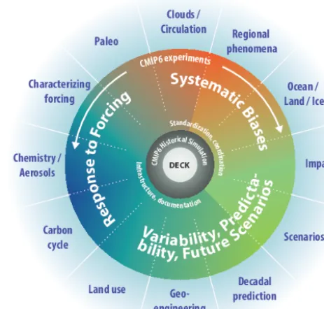
Figure 2.Schematic of the CMIP/CMIP6 experiment design. The inner ring and surrounding white text involve standardized func-tions of all CMIP DECK experiments and the CMIP6 historical simulation. The middle ring shows science topics related specifi-cally to CMIP6 that are addressed by the CMIP6-Endorsed MIPs, with MIP topics shown in the outer ring. This framework is super-imposed on the scientific backdrop for CMIP6 which are the seven WCRP Grand Science Challenges.
These GCs will be using the full spectrum of observa-tional, modelling and analytical expertise across the WCRP, and in terms of modelling most GCs will address their spe-cific science questions through a hierarchy of numerical models of different complexities. Global coupled models ob-viously constitute an essential element of this hierarchy, and CMIP6 experiments will play a prominent role across all GCs by helping to answer the following three CMIP6 science questions: How does the Earth system respond to forcing? What are the origins and consequences of systematic model biases? How can we assess future climate change given inter-nal climate variability, climate predictability, and uncertain-ties in scenarios?
These three questions will be at the centre of CMIP6. Sci-ence topics related specifically to CMIP6 will be addressed through a range of CMIP6-Endorsed MIPs that are organized by the respective communities and overseen by the CMIP Panel (Fig. 2). Through these different MIPs and their con-nection to the GCs, the goal is to fill some of the main scien-tific gaps of previous CMIP phases. This includes, in particu-lar, facilitating the identification and interpretation of model systematic errors, improving the estimate of radiative forc-ings in past and future climate change simulations, facilitat-ing the identification of robust climate responses to aerosol forcing during the historical period, better accounting of the impact of short-term forcing agents and land use on climate, better understanding the mechanisms of decadal climate vari-ability, along with many other issues not addressed satisfac-torily in CMIP5 (Stouffer et al., 2015). In endorsing a num-ber of these MIPs, the CMIP Panel acted to minimize over-laps among the MIPs and to reduce the burden on modelling groups, while maximizing the scientific complementarity and synergy among the different MIPs.
4.2 The CMIP6-Endorsed MIPs
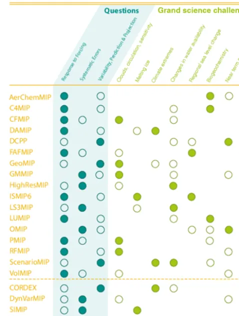
Close to 30 suggestions for CMIP6 MIPs have been re-ceived so far, of which 21 MIPs were eventually endorsed and invited to participate (Table 3). Of those not selected some were asked to work with other proposed MIPs with overlapping science goals and objectives. Of the 21 CMIP6-Endorsed MIPs, 4 are diagnostic in nature, which means that they define and analyse additional output, but do not require additional experiments. In the remaining 17 MIPs, a total of around 190 experiments have been proposed resulting in 40 000 model simulation years with around half of these in Tier 1. The CMIP6-Endorsed MIPs show broad coverage and distribution across the three CMIP6 science questions, and all are linked to the WCRP Grand Science Challenges (Fig. 3).
Each of the 21 CMIP6-Endorsed MIPs is described in a separate invited contribution to this special issue. These con-tributions will detail the goal of the MIP and the major scien-tific gaps the MIP is addressing, and will specify what is new compared to CMIP5 and previous CMIP phases. The
con-Figure 3. Contributions of CMIP6-Endorsed MIPs to the three CMIP6 science questions and the WCRP Grand Science Chal-lenges. A filled circle indicates highest priority and an open circle, second highest priority. Some of the MIPs additionally contribute with lower priority to other CMIP6 science questions or WCRP Grand Science Challenges.
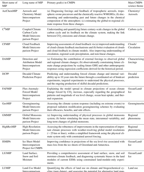
Table 3.List of CMIP6-Endorsed MIPs along with the long name of the MIP, the primary goal(s) and the main CMIP6 science theme as displayed in Fig. 2. Each of these MIPs is described in more detail in a separate contribution to this special issue. MIPs marked with∗are diagnostic MIPs.
Short name of MIP
Long name of MIP Primary goal(s) in CMIP6 Main CMIP6 science theme AerChemMIP Aerosols and
Chemistry Model Intercomparison Project
(a) Diagnosing forcings and feedback of tropospheric aerosols, tropo-spheric ozone precursors and the chemically reactive WMGHGs; (b) doc-umenting and understanding past and future changes in the chemical composition of the atmosphere; (c) estimating the global-to-regional cli-mate response from these changes.
Chemistry/ Aerosols
C4MIP Coupled Climate Carbon Cycle Model Intercom-parison Project
Understanding and quantifying future century-scale changes in the global carbon cycle and its feedback on the climate system, making the link between CO2emissions and climate change.
Carbon cycle
CFMIP Cloud Feedback Model Intercom-parison Project
Improving assessments of cloud feedback via (a) improved understanding of cloud-climate feedback mechanisms and (b) better evaluation of clouds and cloud feedback in climate models. Also improving understanding of circulation, regional-scale precipitation, and non-linear changes.
Clouds/ Circulation
DAMIP Detection and Attribution Model Intercomparison Project
(a) Estimating the contribution of external forcings to observed global and regional climate changes; (b) observationally constraining future cli-mate change projections by scaling future GHG and other anthropogenic responses using regression coefficients derived for the historical period.
Characterizing forcings
DCPP Decadal Climate Prediction Project
Predicting and understanding forced climate change and internal vari-ability up to 10 years into the future through a coordinated set of hindcast experiments, targeted experiments to understand the physical processes, and the ongoing production of skilful decadal predictions.
Decadal prediction
FAFMIP Flux-Anomaly-Forced Model Intercomparison Project
Explaining the model spread in climate projections of ocean climate change forced by CO2increase, especially regarding the geographical
patterns and magnitude of sea level change, ocean heat uptake, and ther-mal expansion.
Ocean/Land/ Ice
GeoMIP Geoengineering Model Intercom-parison Project
Assessing the climate system response (including on extreme events) to proposed radiation modification geoengineering schemes by evaluating their efficacies, benefits, and side effects.
Geoengineering
GMMIP Global Monsoons Model Intercom-parison Project
(a) Improving understanding of physical processes in global monsoons system; (b) better simulating the mean state, interannual variability, and long-term changes of global monsoons.
Regional phenomena
HighResMIP High-Resolution Model Intercom-parison Project
Assessing the robustness of improvements in the representation of impor-tant climate processes with weather-resolving global model resolutions (∼25 km or finer), within a simplified framework using the physical cli-mate system only with constrained aerosol forcing.
Regional phenomena
ISMIP6 Ice Sheet Model Intercomparison Project for CMIP6
Improving confidence in projections of the sea level rise associated with mass loss from the ice sheets of Greenland and Antarctica.
Ocean/Land/ Ice
LS3MIP Land Surface, Snow and Soil Moisture
Providing a comprehensive assessment of land surface, snow, and soil moisture-climate feedback, and diagnosing systematic biases in the land modules of current ESMs using constrained land-module-only experi-ments.
Ocean/Land/ Ice
LUMIP Land-Use Model Intercomparison Project
Quantifying the effects of land use on climate and biogeochemical cy-cling (past–future), and assessing the potential for alternative land man-agement strategies to mitigate climate change.
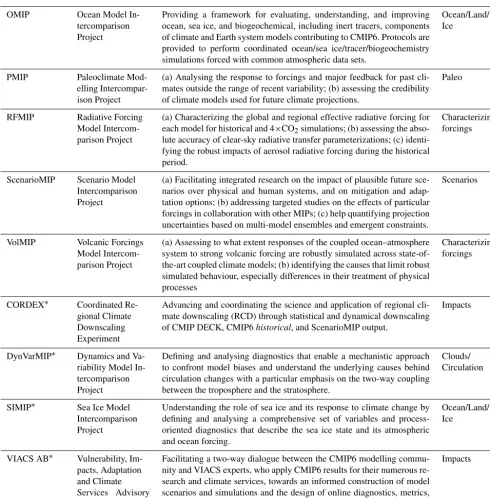
Table 3.Continued.
OMIP Ocean Model In-tercomparison Project
Providing a framework for evaluating, understanding, and improving ocean, sea ice, and biogeochemical, including inert tracers, components of climate and Earth system models contributing to CMIP6. Protocols are provided to perform coordinated ocean/sea ice/tracer/biogeochemistry simulations forced with common atmospheric data sets.
Ocean/Land/ Ice
PMIP Paleoclimate Mod-elling Intercompar-ison Project
(a) Analysing the response to forcings and major feedback for past cli-mates outside the range of recent variability; (b) assessing the credibility of climate models used for future climate projections.
Paleo
RFMIP Radiative Forcing Model Intercom-parison Project
(a) Characterizing the global and regional effective radiative forcing for each model for historical and 4×CO2simulations; (b) assessing the
abso-lute accuracy of clear-sky radiative transfer parameterizations; (c) identi-fying the robust impacts of aerosol radiative forcing during the historical period.
Characterizing forcings
ScenarioMIP Scenario Model Intercomparison Project
(a) Facilitating integrated research on the impact of plausible future sce-narios over physical and human systems, and on mitigation and adap-tation options; (b) addressing targeted studies on the effects of particular forcings in collaboration with other MIPs; (c) help quantifying projection uncertainties based on multi-model ensembles and emergent constraints.
Scenarios
VolMIP Volcanic Forcings Model Intercom-parison Project
(a) Assessing to what extent responses of the coupled ocean–atmosphere system to strong volcanic forcing are robustly simulated across state-of-the-art coupled climate models; (b) identifying the causes that limit robust simulated behaviour, especially differences in their treatment of physical processes
Characterizing forcings
CORDEX∗ Coordinated Re-gional Climate Downscaling Experiment
Advancing and coordinating the science and application of regional cli-mate downscaling (RCD) through statistical and dynamical downscaling of CMIP DECK, CMIP6historical, and ScenarioMIP output.
Impacts
DynVarMIP∗ Dynamics and Va-riability Model In-tercomparison Project
Defining and analysing diagnostics that enable a mechanistic approach to confront model biases and understand the underlying causes behind circulation changes with a particular emphasis on the two-way coupling between the troposphere and the stratosphere.
Clouds/ Circulation
SIMIP∗ Sea Ice Model Intercomparison Project
Understanding the role of sea ice and its response to climate change by defining and analysing a comprehensive set of variables and process-oriented diagnostics that describe the sea ice state and its atmospheric and ocean forcing.
Ocean/Land/ Ice
VIACS AB∗ Vulnerability, Im-pacts, Adaptation and Climate Services Advisory Board
Facilitating a two-way dialogue between the CMIP6 modelling commu-nity and VIACS experts, who apply CMIP6 results for their numerous re-search and climate services, towards an informed construction of model scenarios and simulations and the design of online diagnostics, metrics, and visualization of relevance to society.
Impacts
A number of MIPs are developments and/or continuation of long-standing science themes. These include MIPs specif-ically addressing science questions related to cloud feedback and the understanding of spatial patterns of circulation and precipitation (CFMIP), carbon cycle feedback, and the un-derstanding of changes in carbon fluxes and stores (C4MIP), detection and attribution (DAMIP) that newly includes 21st-century GHG-only simulations allowing the projected re-sponses to GHGs and other forcings to be separated and scaled to derive observationally constrained projections, and
ocean heat uptake and sea level rise (FAFMIP), and under-standing of model response to volcanic forcing (VolMIP).
Since CMIP5, other MIPs have emerged as the modelling community has developed more complex ESMs with inter-active components beyond the carbon cycle. These include the consistent quantification of forcings and feedback from aerosols and atmospheric chemistry (AerChemMIP), and, for the first time in CMIP, modelling of sea level rise from land ice sheets (ISMIP6).
Some MIPs specifically target systematic biases focusing on improved understanding of the sea ice state and its at-mospheric and oceanic forcing (SIMIP), the physical and biogeochemical aspects of the ocean (OMIP), land, snow and soil moisture processes (LS3MIP), and improved un-derstanding of circulation and variability with a focus on stratosphere–troposphere coupling (DynVarMIP). With the increased emphasis in the climate science community on the need to represent and understand changes in regional circula-tion, systematic biases are also addressed on a more regional scale by the Global Monsoon MIP (GMMIP) and a first coordinated activity on high-resolution modelling (High-ResMIP).
For the first time, future scenario experiments, previously coordinated centrally as part of the CMIP5 core experiments, will be run as an MIP ensuring clear definition and well-coordinated science questions. ScenarioMIP will run a new set of future long-term (century timescale) integrations en-gaging input from both the climate science and integrated assessment modelling communities. The new scenarios are based on a matrix that uses the shared socioeconomic path-ways (SSPs, O’Neill et al., 2015) and forcing levels of the Representative Concentration Pathways (RCP) as axes. As a set, they span the same range as the CMIP5 RCPs (Moss et al., 2010), but fill critical gaps for intermediate forcing levels and questions, for example, on short-lived species and land use. The near-term experiments (10–30 years) are coordi-nated by the decadal climate prediction project (DCPP) with improvements expected, for example, from the initialization of additional components beyond the ocean and from a more detailed process understanding and evaluation of the predic-tions to better identify sources and limits of predictability.
Other MIPs include specific future mitigation options, e.g. the land use MIP (LUMIP) that is for the first time in CMIP isolating regional land management strategies to study how different surface types respond to climate change and di-rect anthropogenic modifications, or the geoengineering MIP (GeoMIP), which examines climate impacts of newly pro-posed radiation modification geoengineering strategies.
The diagnostic MIP CORDEX will oversee the downscal-ing of CMIP6 models for regional climate projections. An-other historic development in our field that provides, for the first time in CMIP, an avenue for a more formal communi-cation between the climate modelling and user community is the endorsement of the vulnerability, impacts, and adapta-tion and climate services advisory board (VIACS AB). This
diagnostic MIP requests certain key variables of interest to the VIACS community be delivered in a timely manner to be used by climate services and in impact studies.
All MIPs define output streams in the centrally coordi-nated CMIP6 data request for each of their own experiments as well as the DECK and CMIP6 historical simulations (see the CMIP6 data request contribution to this special issue for details). This will ensure that the required variables are stored at the frequency and resolution required to address the spe-cific science questions and evaluation needs of each MIP and to enable a broad characterization of the performance of the CMIP6 models.
We note that only the Tier 1 MIP experiments are overseen by the CMIP Panel, but additional experiments are proposed by the MIPs in Tiers 2 and 3. We encourage the modelling groups to participate in the full suite of experiments beyond Tier 1 to address in more depth the scientific questions posed. The call for MIP applications for CMIP6 is still open and new proposals will be reviewed at the annual WGCM meet-ings. However, we point out that the additional MIPs sug-gested after the CMIP6 data request has been finalized will have to work with the already defined model output from the DECK and CMIP6 historical simulations, or work with the modelling group to recover additional variables from their internal archives. We also point out that some experiments proposed by CMIP6-Endorsed MIPs may not be finished un-til after CMIP6 ends.
5 Summary
CMIP6 continues the pattern of evolution and adaptation characteristic of previous phases of CMIP. To centre CMIP at the heart of activities within climate science and encourage links among activities within the World Climate Research Programme (WCRP), CMIP6 has been formulated scientif-ically around three specific questions, amidst the backdrop of the WCRP’s seven Grand Science Challenges. To meet the increasingly broad scientific demands of the climate-science community, yet be responsive to the individual prior-ities and resource limitations of the modelling centres, CMIP has adopted a new, more federated organizational structure.
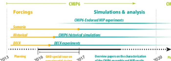
forc-Figure 4.CMIP6 timeline for the preparation of forcings, the realization of experiments and their analysis.
ing, from how the terrestrial biosphere influences the uptake of CO2 to how much predictability is stored in the ocean,
from how to best project near-term to long-term future cli-mate changes while considering interdependence and differ-ences in model performance in the CMIP6 ensemble, and from what regulates the distribution of tropospheric ozone, to the influence of land-use changes on water availability.
The last 3 years have been dedicated to conceiving and then planning what we now call CMIP6. Starting in 2016, the first modelling centres are expected to begin performing the DECK and uploading output on the ESGF. Forcings for the DECK and CMIP6 historical simulations will be ready be-fore mid-2016 so that these experiements can be started, and by the end of 2016 the diverse forcings for different scenarios of future human activity will become available. Past experi-ence suggests that most centres will complete their CMIP simulations within a few years while the analysis of CMIP6 results will likely go on for a decade or more (Fig. 4).
Through an intensified effort to align CMIP with spe-cific scientific questions and the WCRP Grand Science Chal-lenges, we expect CMIP6 to continue CMIP’s tradition of major scientific advances. CMIP6 simulations and scientific achievements are expected to support the IPCC Sixth Assess-ment Report (AR6) as well as other national and international climate assessments or special reports. Ultimately scientific progress on the most pressing problems of climate variability and change will be the best measure of the success of CMIP6.
Data availability
Appendix A: Experiment specifications A1 Specifications for the DECK
Here we provide information needed to perform the DECK, including specification of forcing and boundary conditions, initialization procedures, and minimum length of runs. This information is largely consistent with but not identical to the specifications for these experiments in CMIP5 (Taylor et al., 2009).
The DECK and CMIP6 historical simulations are re-quested from all models participating in CMIP. The expec-tation is that this requirement will be met for each model configuration used in the subsequent CMIP6-Endorsed MIPs (an entry card). For CMIP6, in the special case where the burden of the entry card simulations is prohibitive but the scientific case for including a particular model simulation is compelling (despite only partial completion of the entry card simulations), an exception to this policy can be granted on a model-by-model basis by the CMIP Panel, which will seek advice from the chairs of the affected CMIP6-Endorsed MIP. CMIP6 is a cooperative effort across the international cli-mate modelling and clicli-mate science communities. The mod-elling groups have all been involved in the design and imple-mentation of CMIP6, and thus have agreed to a set of best practices proposed for CMIP6. Those best practices include having the modelling groups submit the DECK experiments and the CMIP6 historical simulations to the ESGF, as well as any CMIP6-Endorsed MIP experiments they choose to run. Additionally, the modelling groups decide what constitutes a new model version. The CMIP Panel will work with the MIP co-chairs and the modelling groups to ensure that these best practices are followed.
A1.1 AMIP simulation
As in the first simulations performed under the Atmospheric Model Intercomparison Project (AMIP, Gates et al., 1999), SSTs and SICs in AMIP experiments are prescribed con-sistent with observations (see details on this forcing data set in the corresponding contribution to this special issue). Land models should be configured as close as possible to the one used in the CMIP6 historical simulation including tran-sient land use and land cover. Other external forcings includ-ing volcanic aerosols, solar variability, GHG concentrations, and anthropogenic aerosols should also be prescribed consis-tent with those used in the CMIP6 historical simulation (see Sect. A2 below). Even though in AMIP simulations models with an active carbon cycle will not be fully interactive, sur-face carbon fluxes should be archived over land.
AMIP integrations can be initialized from prior model in-tegrations or from observations or in other reasonable ways. Depending on the treatment of snow cover, soil water con-tent, the carbon cycle, and vegetation, these runs may require a spin-up period of several years. One might establish
quasi-equilibrium conditions consistent with the model by, for ex-ample, running with ocean conditions starting earlier in the 1970s or cycling repeatedly through year 1979 before simu-lating the official period. Results from the spin-up period (i.e. prior to 1979) should be discarded, but the spin-up technique should be documented.
For CMIP6, AMIP simulations should cover at least the period from January 1979 through December 2014, but mod-elling groups are encouraged to extend their runs to the end of the observed period. Output may also be contributed from years preceding 1979 with the understanding that surface ocean conditions were less complete and in some cases less reliable then.
The climate found in AMIP simulations is largely de-termined by the externally imposed forcing, especially the ocean conditions. Nevertheless, unforced variability (noise) within the atmosphere introduces some non-deterministic variations that hamper unambiguous interpretation of ap-parent relationships between, for example, the year-to-year anomalies in SSTs and their consequences over land. To as-sess the role of unforced atmospheric variability in any par-ticular result, modelling groups are encouraged to generate an ensemble of AMIP simulations. For most studies, a three-member ensemble, where only the initial conditions are var-ied, would be the minimum required, with larger size ensem-bles clearly of value in making more precise determination of statistical significance.
A1.2 Multi-century pre-industrial control simulations Like laboratory experiments, numerical experiments are de-signed to reveal cause and effect relationships. A standard way of doing this is to perform both a control experiment and a second experiment where some externally imposed ex-periment condition has been altered. For many CMIP experi-ments, including the rest of the experiments discussed in this Appendix, the control is a simulation with atmospheric com-position and other conditions prescribed and held constant, consistent with best estimates of the forcing from the histor-ical period.
piControl-spinuporesm-piControl-spinup). At the very least the length of the spin-up period should be documented.
Although equilibrium is generally not achieved, the changes occurring after the spin-up period are usually found to evolve at a fairly constant rate that presumably decreases slowly as equilibrium is approached. After a few centuries, these drifts of the system mainly affect the carbon cycle and ocean below the main thermocline, but they are also manifest at the surface in a slow change in sea level. The climate drift must be removed in order to interpret experiments that use the pre-industrial simulation as a control. The usual proce-dure is to assume that the drift is insensitive to CMIP exper-iment conditions and to simply subtract the control run from the perturbed run to determine the climate change that would occur in the absence of drift.
Besides serving as controls for numerical experimentation, thepiControlandesm-piControlare used to study the natu-rally occurring, unforced variability of the climate system. The only source of climate variability in a control arises from processes internal to the model, whereas in the more complicated real world, variations are also caused by exter-nal forcing factors such as solar variability and changes in atmospheric composition caused, for example, by human ac-tivities or volcanic eruptions. Consequently, the physical pro-cesses responsible for unforced variability can more easily be isolated and studied using the control run of models, rather than by analysing observations.
A DECK control simulation is required to be long enough to extend to the end of any perturbation runs initiated from it so that climate drift can be assessed and possibly removed from those runs. If, for example, a historical simulation (be-ginning in 1850) were initiated from the be(be-ginning of the control simulation and then were followed by a future sce-nario run extending to year 2300, a control run of at least 450 years would be required. As discussed above, control runs are also used to assess model-simulated unforced cli-mate variability. The longer the control, the more precisely can variability be quantified for any given timescale. A con-trol simulation of many hundreds of years would be needed to assess variability on centennial timescales. For CMIP6 it is recommended that the control run should be at least 500 years long (following the spin-up period), but of course the simulation must be long enough to reach to the end of the experiments it spawns. It should be noted that those analysing CMIP6 simulations might also require simulations longer than 500 years to accurately assess unforced variabil-ity on long timescales, so modelling groups are encouraged to extend their control runs well beyond the minimum rec-ommended number of years.
Because the climate was very likely not in equilibrium with the forcing of 1850 and because different components of the climate system differentially respond to the effects of the forcing prior to that time, there is some ambiguity in de-ciding on what forcing to apply for the control. For CMIP6
we recommend a specification of this forcing that attempts to balance conflicting objectives to
– minimize artificial climate responses to discontinuities in radiative forcing at the time a historical simulation is initiated, and
– minimize artefacts in sea level change due to thermal expansion caused by unrealistic mismatches in condi-tions in the centennial-scale averaged forcings for the pre- and post-1850 periods. Note that any preindus-trial multi-centennial observed trend in global-mean sea level is most likely to be due to slow changes in ice-sheets, which are likely not to be simulated in the CMIP6 model generation.
The first consideration above implies that radiative forcing in the control run should be close to that imposed at the be-ginning of the CMIP historical simulation (i.e. 1850). The second implies that a background volcanic aerosol and time-averaged solar forcing should be prescribed in the control run, since to neglect it would cause an apparent drift in sea level associated with the suppression of heat uptake due to the net effect of, for instance, volcanism after 1850, and this has implications for sea level changes (Gregory, 2010; Gre-gory et al., 2013). We recognize that it will be impossible to entirely avoid artefacts and artificial transient effects, and practical considerations may rule out conformance with ev-ery detail of the control simulation protocol stipulated here. With that understanding, here is a summary of the recom-mendations for the imposed conditions on the spin-up and control runs, followed by further clarification in subsequent paragraphs:
– Conditions must be time invariant except for those asso-ciated with the mean climate (notably the seasonal and diurnal cycles of insolation).
– Unless indicated otherwise (e.g. the background vol-canic forcing), experiment conditions (e.g. greenhouse gas concentrations, ozone concentration, surface land conditions) should be representative of Earth around the year 1850.
– Orbital parameters (eccentricity, obliquity, and longi-tude of the perihelion) should be held fixed at their 1850 values.
– Land use should not change in the control run and should be fixed according to reconstructed agricultural maps from 1850. Due to the diversity of model ap-proaches in ESMs for land carbon, some groups might deviate from this specification, and again this must be clearly documented.
– A background volcanic aerosol should be specified that results in radiative forcing matching, as closely as pos-sible, that experienced, on average, during the historical simulation (i.e. 1850–2014 mean).
– Models without interactive ozone chemistry should specify the pre-industrial ozone fields from a data set produced from a pre-industrial control simulation that uses 1850 emissions and a mean solar forcing averaged over solar cycles 8–10, representative of the mean mid-19th century solar forcing.
– For models with interactive chemistry and/or aerosols, the CMIP6 pre-industrial emissions dataset of reactive gases and aerosol precursors should be used. For models without internally calculated aerosol concentrations, a monthly climatological dataset of aerosol physical and optical properties should be used.
In the CO2-concentration-drivenpiControl, the value of the
global annual mean 1850 atmospheric CO2concentration is
prescribed and held fixed during the entire experiment. There are some special considerations that apply to control simula-tions performed by emission-driven ESMs (i.e. runs with at-mospheric concentrations of CO2 calculated prognostically
rather than being prescribed). In theesm-piControl simula-tion, emissions of CO2from both fossil fuel combustion and
land-use change are prescribed to be zero. In this run any residual drift in atmospheric CO2 concentration that arises
from an imbalance in the exchanges of CO2between the
at-mosphere and the ocean and land (i.e. by the natural carbon cycle in the absence of anthropogenic CO2 emissions) will
need to be subtracted from perturbation runs to correct for a control state not in equilibrium. It should be emphasized that theesm-piControlis an idealized experiment and is not meant to mimic the true 1850 conditions, which would have to include a source of carbon of around 0.6 Pg C yr−1 from the already perturbed state that existed in 1850.
Due to a wide variety of ESMs and the techniques they use to compute land carbon fluxes, it is hard to make statements that apply to all models equally well. A general recommen-dation, however, is that the land carbon fluxes in the emission and concentration-driven control simulations should be sta-ble in time and in approximate balance so that the net carbon flux into the atmosphere is small (less than 0.1 Pg C yr−1). Further details on ESM experiments with a carbon cycle are provided in the C4MIP contribution to this special issue.
The historical time-average volcanic forcing stipulated above for the control run is likely to approximate the much longer term mean. The volcanic aerosol radiative forcing es-timates of Crowley (2000) for the historical period and the last millennium are −0.18 and −0.22 W m−2, respectively. Because the mean volcanic forcing between 1850 and 2014 is small, the discontinuity associated with transitioning from a mean forcing to a time-varying volcanic forcing is also ex-pected to be small. Even though this is the design objective, it
is likely that it will be impossible to eliminate all artefacts in quantities such as historical sea level change. For this reason, and because some models may deviate from these specifica-tions, it is recommended that groups perform an additional simulation of the historical period but with only natural forc-ing included. With this additional run, which is already called for under DAMIP, the purely anthropogenic effects on sea level change can be isolated.
The forcing specified in the piControl also has implica-tions for simulaimplica-tions of the future, when solar variability and volcanic activity will continue to exist, but at unknown lev-els. These issues need to be borne in mind when designing and evaluating future scenarios, as a failure to include vol-canic forcing in the future will cause future warming and sea level rise to be over-estimated relative to apiControl ex-periment in which a non-zero volcanic forcing is specified. This is accounted for by introducing a time-invariant non-zero volcanic forcing (e.g. the mean volcanic forcing for the piControl) into the scenarios. This is further specified in the ScenarioMIP contribution to this special issue.
These issues, and the potential of different modelling cen-tres adopting different approaches to account for their partic-ular constraints, highlight the paramount importance of ade-quately documenting the conditions under which this and the other DECK experiments are performed.
A1.3 Abruptly quadrupling CO2simulation
Until CMIP5, there were no experiments designed to quan-tify the extent to which forcing differences might explain differences in climate response. It was also difficult to diag-nose and quantify the feedback responses, which are medi-ated by global surface temperature change (Sherwood et al., 2015). In order to examine these fundamental characteristics of models – CO2forcing and climate feedback – an abrupt
4×CO2 simulation was included for the first time as part
of CMIP5. Following Gregory et al. (2004), the simulation branches in January of the CO2-concentration-driven
piCon-troland abruptly the value of the global annual mean 1850 atmospheric CO2concentration that is prescribed in
piCon-trolis quadrupled and held fixed. As the system subsequently evolves toward a new equilibrium, the imbalance in the net flux at the top of the atmosphere can be plotted against global temperature change. As Gregory et al. (2004) showed, it is then possible to diagnose both the effective radiative forc-ing due to a quadruplforc-ing of CO2and also effective
equilib-rium climate sensitivity (ECS). Moreover, by examining how individual flux components evolve with surface temperature change, one can learn about the relative strengths of differ-ent feedback, notably quantifying the importance of various feedback associated with clouds.
In theabrupt-4×CO2experiment, the only externally im-posed difference from the piControl should be the change in CO2concentration. All other conditions should remain as
vol-canic aerosols. By changing only a single factor, we can un-ambiguously attribute all climatic consequences to the in-crease in CO2concentration.
The minimum length of the simulation should be 150 years, but longer simulations would enable investiga-tions of longer-timescale responses. Also there is value, as in CMIP5, in performing an ensemble of short (∼5-year) simu-lations, all prescribing global annual mean 1850 atmospheric CO2concentration but initiated at different times throughout
the year (in addition to theabrupt-4×CO2simulation initi-ated from thepiControlin January). Such an ensemble would reduce the statistical uncertainty with which the effective CO2 radiative forcing could be quantified and would allow
more detailed and accurate diagnosis of the fast responses of the system under an abrupt change in forcing (Bony et al., 2013; Gregory and Webb, 2008; Kamae and Watanabe, 2013; Sherwood et al., 2015). Different groups will be able to afford ensembles of different sizes, but in any case each realization should be initialized in a different month and the months should be spaced evenly throughout the year.
A1.4 1 % CO2increase simulation
The second idealized climate change experiment was intro-duced in the early days of CMIP (Meehl et al., 2000). It is designed for studying model responses under simplified but somewhat more realistic forcing than an abrupt increase in CO2. In this1pctCO2experiment, the simulation is branched
from thepiControl, and the global annual mean CO2
concen-tration is gradually increased at a rate of 1 % yr−1(i.e. expo-nentially), starting from its 1850 value that is prescribed in thepiControl. A minimum length of 150 years is requested so that the simulation goes beyond the quadrupling of CO2
after 140 years. Note that in contrast to previous definitions, the experiment has been simplified so that the 1 % CO2
in-crease per year is applied throughout the entire simulation rather than keeping it constant after 140 years as in CMIP5. Since the radiative forcing is approximately proportional to the logarithm of the CO2increase, the radiative forcing
lin-early increases over time. Drawing on the estimates of ef-fective radiative forcing (for definitions see Myhre et al., 2013) obtained in the abrupt-4×CO2 simulations, analysts can scale results from each model in the 1 % CO2increase
simulations to focus on the response differences in models, largely independent of their forcing differences. In contrast, in CMIP6 historical simulations (see Sect. A2), the forcing and response contributions to model differences in simulated climate change cannot be easily isolated.
As in theabrupt-4×CO2experiment, the only externally imposed difference from thepiControlshould be the change in CO2 concentration. The omission of changes in aerosol
concentrations is the key to making these simulations easier to interpret.
Models with a carbon cycle component will be driven by prescribed CO2concentrations, but terrestrial and marine
surface fluxes and stores of carbon will become a key diag-nostic from which one can infer emission rates that are con-sistent with a 1 % yr−1increase in model CO2concentration.
This DECK baseline carbon cycle experiment is built upon in C4MIP to diagnose the strength of model carbon climate feedback and to quantify contributions to disruption of the carbon cycle by climate and by direct effects of increased CO2concentration.
A2 The CMIP6 historical simulations
CMIP6 historical simulations of climate change over the pe-riod 1850–2014 are forced by common data sets that are largely based on observations. They serve as an important benchmark for assessing model performance through evalu-ation against observevalu-ations. The historical integrevalu-ation should be initialized from some point in the control integration (with historical branching from the piControl and the esm-hist branching from esm-piControl) and be forced by varying time, externally imposed conditions that are based on obser-vations. Both naturally forced changes (e.g. due to solar vari-ability and volcanic aerosols) and changes due to human ac-tivities (e.g. CO2concentration, aerosols, and land use) will
lead to climate variations and evolution. In addition, there is unforced variability which can obscure the forced changes and lead to expected differences between the simulated and observed climate variations (Deser et al., 2012).
The externally imposed forcing data sets that should be used in CMIP6 cover the period 1850 through the end of 2014 and are described in detail in various other contribu-tions to this special issue. In the CO2-concentration-driven
historical simulations, time-varying global annual mean con-centrations for CO2 and other long-lived greenhouse gases
are prescribed. If a modelling center decides to represent ad-ditional spatial and seasonal variations in prescribed green-house gas forcings, this needs to be adequately documented. Recall from Sect. A1.2 that the conditions in the control should generally be consistent with the forcing imposed near the beginning of the CMIP historical simulation. This should minimize artificial transient effects in the first portion of the CMIP historical simulation. An exception is that for the CO2
-emission-driven experiments, the zero CO2emissions from
fossil fuel and the land-use specifications for 1850 in the esm-piControlcould cause a discontinuity in land carbon at the branch point.
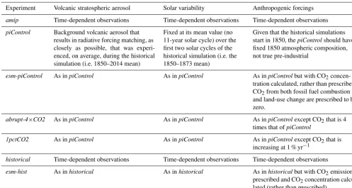
Table A1.Specifications in the DECK and CMIP6 historical simulations.
Experiment Volcanic stratospheric aerosol Solar variability Anthropogenic forcings
amip Time-dependent observations Time-dependent observations Time-dependent observations
piControl Background volcanic aerosol that results in radiative forcing matching, as closely as possible, that was experi-enced, on average, during the historical simulation (i.e. 1850–2014 mean)
Fixed at its mean value (no 11-year solar cycle) over the first two solar cycles of the historical simulation (i.e. the 1850–1873 mean)
Given that the historical simulations start in 1850, thepiControlshould have fixed 1850 atmospheric composition, not true pre-industrial
esm-piControl As inpiControl As inpiControl As inpiControlbut with CO2 concen-tration calculated, rather than prescribed. CO2from both fossil fuel combustion
and land-use change are prescribed to be zero.
abrupt-4×CO2 As inpiControl As inpiControl As inpiControlexcept CO2that is 4
times that ofpiControl
1pctCO2 As inpiControl As inpiControl As inpiControlexcept CO2that is
increasing at 1 % yr−1
historical Time-dependent observations Time-dependent observations Time-dependent observations
esm-hist As inhistorical As inhistorical As inhistoricalbut with CO2emissions
prescribed and CO2concentration
calcu-lated (rather than prescribed)
to account for the land carbon cycle disequilibrium before 1850 and to adequately simulate carbon stores at the start of the historical simulation (Sentman et al., 2011). Due to the wide diversity of modelling approaches for land carbon in the ESMs, the actual method applied by each group to account for these effects will differ and needs to be well documented. As discussed earlier, there will be a mismatch in the spec-ification of volcanic aerosols between control and historical simulations that especially affect estimates of ocean heat up-take and sea level rise in the historical period. This can be minimized by prescribing a background volcanic aerosol in the pre-industrial control that has the same cooling effect as the volcanoes included in the CMIP6 historical simulation. Any residual mismatch will need to be corrected, which re-quires a special supplementary simulation (see Sect. A1.2) that should be submitted along with the CMIP6 historical simulation.
For model evaluation and for detection and attribution studies (the focus of DAMIP) there would be considerable value in extending the CMIP6 historical simulations beyond the nominal 2014 ending date. To include the more recent observations in model evaluation, modelling groups are en-couraged to document and apply forcing data sets represent-ing the post-2014 period. For short extensions (up to a few years) it may be acceptable to simply apply forcing from one of the future scenarios defined by ScenarioMIP. To distin-guish between the portion of the historical period when all models will use the same forcing data sets (i.e. 1850–2014) from the extended period where different data sets might be
used, the experiment for 1850–2014 will be labelled histori-cal(esm-histin the case of the emission-driven run) and the period from 2015 through near-present will likely be labelled historical-ext(esm-hist-ext).
Even if the CMIP6 historical simulations are extended be-yond 2014, all future scenario simulations (called for by Sce-narioMIP and other MIPs) should be initiated from the end of year 2014 of the CMIP6 historical simulation since the “future” in CMIP6 begins in 2015.