doi:10.5194/gmd-5-499-2012
© Author(s) 2012. CC Attribution 3.0 License.
Model Development
A subgrid parameterization scheme for precipitation
S. Turner, J.-L. Brenguier, and C. Lac
Groupe d’Etude de l’Atmosph`ere M´et´eorologique/CNRM-GAME M´et´eo-France, URA1357, 42 Av Gaspard Coriolis, 31057 Toulouse Cedex 1, France
Correspondence to: S. Turner ([email protected])
Received: 19 April 2011 – Published in Geosci. Model Dev. Discuss.: 26 July 2011 Revised: 8 March 2012 – Accepted: 17 March 2012 – Published: 23 April 2012
Abstract. With increasing computing power, the horizontal resolution of numerical weather prediction (NWP) models is improving and today reaches 1 to 5 km. Nevertheless, clouds and precipitation formation are still subgrid scale processes for most cloud types, such as cumulus and stratocumulus. Subgrid scale parameterizations for water vapor condensa-tion have been in use for many years and are based on a prescribed probability density function (PDF) of relative hu-midity spatial variability within the model grid box, thus pro-viding a diagnosis of the cloud fraction. A similar scheme is developed and tested here. It is based on a prescribed PDF of cloud water variability and a threshold value of liq-uid water content for droplet collection to derive a rain frac-tion within the model grid. Precipitafrac-tion of rainwater raises additional concerns relative to the overlap of cloud and rain fractions, however. The scheme is developed following an analysis of data collected during field campaigns in stratocu-mulus (DYCOMS-II) and fair weather custratocu-mulus (RICO) and tested in a 1-D framework against large eddy simulations of these observed cases. The new parameterization is then im-plemented in a 3-D NWP model with a horizontal resolution of 2.5 km to simulate real cases of precipitating cloud sys-tems over France.
1 Introduction
In warm clouds, droplets form on activated cloud condensa-tion nuclei (CCN) and grow by condensacondensa-tion of water vapor. Precipitation occurs when a few droplets grow large enough, typically within the range of 20 to 30 µm radius, for their sedimentation velocity to enhance the probability of colli-sion and coalescence with smaller droplets. Observations have shown that such precipitation embryos are formed when the mean volume droplet radius of the droplet size
distribu-tion reaches a threshold of 10–12 µm (Gerber, 1996; Boers et al., 1998; Pawlowska and Brenguier, 2003). These em-bryos then become more efficient as they grow by collection, and precipitation develops until most of the cloud droplets have been collected (Pruppacher and Klett, 1997). The on-set of precipitation is thus particularly sensitive to the likeli-hood of a few droplets (a few per liter) reaching this thresh-old radius. This depends on the local values of the liquid water content (qc) and droplet number concentration (N), as r=( qc
4π/3ρwN)
1/3. The key issue here is that the onset of pre-cipitation is a small-scale process, typically on the scale of a convective cell core, i.e. a few tens of meters. This pro-cess is well reproduced with Large Eddy Simulations (LES) and bulk microphysics schemes (Khairoutdinov and Kogan, 2000; Stevens et al., 1996; Morrison and Grabowski, 2008), but coarser resolution Numerical Weather Prediction mod-els (NWP) and climate modmod-els have difficulties simulating precipitation formation because clouds occupy only a frac-tion of the grid and the grid mean values of the bulk micro-physical parameters are not representative of the peak values occurring at a few local spots.
Long-term observations of clouds and precipitation made within the framework of the Cloudnet project show that the UK Unified model captures the frequency of occurrence of clouds and precipitation, and the diurnal cycle in cloud height reasonably well, on average (Illingworth et al., 2007; Barrett et al., 2009), but two major shortcomings of the model have also been identified. First, the model underestimates the fre-quency of occurrence of overcast grid boxes by a factor of two; second, values of drizzle rate greater than 0.1 mm h−1 are ten times more frequent in the model than in the observa-tions. Such biases are also observed with the ECMWF and ALADIN models, which show a clear overestimation in light precipitation. The impact is not as strong for surface pre-cipitation since most drizzle evaporates before reaching the ground, but rather for the overall dynamics of the boundary
layer because of the resulting enhanced cooling of the sub-cloud layer, which leads to sub-clouds dissipating too rapidly.
When cloud properties are statistically homogeneous within a model grid (≥50 km), empirical relationships can be derived between precipitation rate at cloud base, cloud liquid water path (LWP) and the mean value of the concentration of activated nuclei (Nact). Such relationships were initially derived from field experiments such as ACE-2 (Pawlowska and Brenguier, 2003), EPIC (Comstock et al., 2004) and DYCOMS-II (van Zanten et al., 2005), and they have been further corroborated by LES simulations of stratocumulus (Geoffroy et al., 2008) and cumulus fields (Jiang et al., 2010). At higher horizontal resolutions, however, only few clouds occupy the model grid, and such a statistical approach is no longer valid.
The issue is analogous to the simulation of water vapor condensation, which called for the implementation of sub-grid cloud schemes (Sommeria and Deardorf, 1977): the rel-ative humidity fluctuations in a model grid are represented by a Probability Density Function (PDF) specified a priori and the fraction of the PDF with humidity values greater than 100 % determines the cloud fraction (CF). With such an artifice, the transition from clear to fully cloudy grids is smoothed out and the non-linear interactions (radiation for instance) are better represented. For radiative transfer calcu-lations, however, additional hypotheses are necessary to ver-tically overlap the cloud fractions diagnosed independently at each model level.
Similarly, subgrid rain schemes aim at simulating the grad-ual transition from non-precipitating to fully precipitating model grids. Because of the non-linearity of the onset of precipitation, such a scheme is expected to significantly im-pact simulations of shallow convective clouds in which the grid mean values of the droplet mean volume diameter hardly reach the collection threshold while local values might.
Subgrid schemes thus attempt to calculate the grid mean impact of non-linear physical processes when the grid mean values of the state parameters are specified. In a statistical approach, the key issue is therefore to select universal distri-butions to represent the subgrid variability of the atmospheric state parameters. The challenge is that such distributions are not statistically independent since many cloud processes de-pend on their joint variability. For instance, dede-pends jointly on temperature and humidity through relative humidity, but more precisely on their joint variability, which determines the probability of the relative humidity reaching 100 % in a model grid. Parameterization of precipitation introduces an additional level of complexity since the rate of droplet ac-cretion by drops depends on the product of the cloud and precipitating water mixing ratios.
A few alternative approaches have therefore been explored to get around this problem, in which the equations are al-lowed to build the convective structures but in a simpli-fied two-dimensional framework. These approaches are re-ferred to as superparameterization (Grabowski, 1999),
quasi-3-D Multi-scale Modeling Framework (Arakawa, 2004), or Macro-Micro-Interlocked algorithm (Kusano et al., 2007).
Within the framework of the statistical approach, new techniques have also been developed to stochastically sample the possible states of the system with the purpose of decreas-ing the cost of the parameterization without reducdecreas-ing its level of complexity. They include the Joint PDF approach of Golaz et al. (2002), the generation of a cloudy sub-column with Full Generator (FGen) by R¨ais¨anen et al. (2004), precipitation formation using the Latin Hypercube Sampling by Larson et al. (2005), the cellular automatons of Berner (2005), and the stochastic activation of convection by Tompkins (2005).
The scheme tested here is based on the PDF approach in-troduced by Sommeria and Deardorff (1977), which has been extensively used for subgrid condensation (Bougeault, 1981; Tompkins, 2002; Bony and Emanuel, 2001). The onset of precipitation still relies on the mean cloud fraction value of the cloud water content while, locally, peak values can reach the collection threshold and initiate precipitation before the mean value is reached. Following Bechtold et al. (1993), the variability of the cloud water content in the cloud fraction of a model grid is represented by a PDF and precipitation is initiated in the subcloud fraction where the values of the cloud water content are greater than the collection thresh-old. This cloud water splitting for rain formation is similar to the Tripleclouds scheme developed for radiation purposes by Shonk and Hogan (2008), although the splitting is not ar-bitrarily specified here but depends rather on the comparison with the threshold radius for collection.
The modeling context is described in the following section with more details on the bulk microphysics scheme. After a presentation of the subgrid parameterization of precipitation in Sect. 3, two boundary layer cases of stratocumulus and cumulus clouds will be used to compare observations with LES and SCM (single column model) simulations in Sects. 4 and 5, respectively. The results obtained with the research model for a real (3-D) case of precipitating boundary layer clouds are presented in Sect. 6, followed by our conclusions.
2 Modeling context and methodology
The horizontal resolution of most of current state-of-the-art operational mesoscale forecast models now reaches 1–5 km, which allows to explicitly resolve cloud structures. In NWP mesoscale models, single moment bulk microphysics param-eterizations are currently used for precipitation processes, with mixing ratios of the different species as prognostic vari-ables. If the impacts of aerosols on clouds (aerosol indi-rect effects) are to be accounted for, double moment schemes have to be used, with additional variables for the number con-centrations of cloud and precipitation particles.
This study was done to improve small-scale precipitations for M´et´eo-France NWP model AROME (2.5 km, Seity et al., 2011). The parameterizations of the physical processes are
derived from those developed for the non-hydrostatic anelas-tic research model Meso-NH (Lafore et al., 1998), while the dynamical core comes from the regional ALADIN non-hydrostatic operational model (Bubnova et al., 1995). The AROME and Meso-NH models use a statistical subgrid con-densation scheme to diagnose the cloud fraction using sub-grid scale cloud variability from the turbulence (Bougeault, 1982; Bechtold et al., 1995) and the shallow convection scheme (Pergaud et al., 2009). Both models use the ICE3 single moment microphysical scheme (Pinty and Jabouille, 1998). The subgrid precipitation scheme is tested in this framework, but limited to warm precipitation, although it can be extended to mixed microphysics and adapted to double moment schemes.
The development of a PDF-type subgrid scheme raises two issues: first the selection of a universal function for the PDF that realistically reflects statistical distribution of the small scale microphysical parameter values and, second, the defi-nition of rules for the vertical overlap of the subgrid fractions, cloudy and clear air fractions and, inside the cloudy fraction, the precipitating and non-precipitating fractions.
The first issue is addressed by analyzing airborne data collected in shallow convective clouds, stratocumulus (DYCOMS-II) and cumulus (RICO). Airborne data, how-ever, covers a very limited fraction of the domain. To ex-tend the 3-dimensional characterization of the microphysical fields, LES are performed with the Meso-NH model. Af-ter validation of the simulations against the observations, the simulated fields are used to complement the statistics. 2.1 The Meso-NH LES simulations
The DYCOMS-II and RICO cases were run using the LES version of Meso-NH with a timestep of 1 s and fine horizontal and vertical resolutions (see Table 1). The turbulent scheme was a 3-D turbulent kinetic energy (TKE) scheme (Cuxart et al., 2000) with a Deardorff mixing length. PBL clouds were assumed to be resolved at the LES resolution with “all or nothing” condensation. Microphysical schemes were ei-ther the one-moment scheme of Pinty and Jabouille (1998), also referred to as the ICE3 or SM (Single Moment) scheme, or the two-moment scheme of Cohard and Pinty (2000), re-ferred to as the C2R2 scheme, or the scheme by Geoffroy et al. (2008), also referred to as the KHKO scheme (both two-moment schemes will be further referenced as DM, Double Moment). The DM scheme rely on four prognostic vari-ables: the cloud droplet and drizzle/rain drop concentration, and the cloud droplet and drizzle/rain drop mixing ratios. A fifth prognostic variable is used to account for already activated CCN, following the activation scheme of Cohard et al. (1998), which is an extension of the Twomey (1959) parameterization for more realistic activation spectra. The number of CCN, activated at any time step, is equal to the difference between the number of CCN which would activate at the diagnosed pseudo-equilibrium peak supersaturation in
the grid (depending on updraft velocity and temperature) and the concentration of already activated aerosols. DM simula-tions were performed here with activation spectra producing concentrations of activated nuclei at 1 % supersaturation of 50, 70, and 100 cm−3, called DM-50, DM-70 and DM-100, respectively.
2.2 The Meso-NH SCM simulations
In order to test the new parameterization for operational mesoscale models (1–5 km), the Meso-NH model was also used in a single column (SCM) mode initialized with the same forcing fields as for the DYCOMS-II and RICO LES. Table 1 shows some differences between LES and SCM sim-ulations. The SM scheme was used in all SCM simulations, without (SM-CTRL) or with (SM-NEW) the new subgrid rain parameterization.
3 Subgrid rain parameterization scheme
The Meso-NH model already uses a subgrid scheme for cloud fraction (CF). Note, however, that the new scheme will also work without a cloud fraction scheme (CF = 1), al-though the potential benefits would probably be limited in such cases.
3.1 Splitting of the cloud water PDF
We defined the local value of the cloud water content (CWC) in the cloudy fraction asq˜c= ¯qc/CF, whereq¯c is the grid mean value in the model. In the cloud fraction, the CWC PDF was represented by an analytical function (f(q˜c))with one parameter that was constrained by its first moment,q˜c. The cloudy fraction was then divided into two parts, in which the local values of the cloud water mixing ratio were respec-tively lower (CFL) and higher (CFH) than the autoconversion threshold of the microphysical scheme (see Appendix A for the values of the autoconversion scheme used in this study). The CWC mean values in the CFLand CFHsubcloud frac-tions are defined as for the first moment of the PDF, wereq˜cL is integrated from 0 to the collection thresholdqcR, which can be of Kessler type or any other one, andq˜cHis the inte-gration of all values higher thanqcR. The grid mean values were similarly split in two parts:
CF=CFH+CFL (1)
¯
qc= ¯qcH+ ¯qcL (2)
By definition, there is no production of precipitating particles in CFLand the autoconversion scheme (Kessler, 1969) was only applied in CFHwith a CWC value equal toq˜cH.
3.2 The cloud water PDF
Statistics of cumulus CWC derived from past observations and LES cases suggest that linear or quadratic decreasing
Table 1. Set-up for LES and SCM simulations of DYCOMS-II and RICO.
DYCOMS-II Simulations RICO Simulations LES (3-D) SCM (1-D) LES (3-D) SCM (1-D)
Horizontal resolution 50 m 2.5 km 100 m 2.5 km Number of grid points 128×128 1×1 128×128 1×1
Horizontal domain 6.4 km – 12.8 km –
Vertical resolution 10 m 10 m 40 m 40 m
Number of levels 150 150 100 100
Domain height 1.5 km 1.5 km 4 km 4 km
Timestep 1 s 10 s 1 s 10 s
Total duration 6 h 6 h 24 h 24 h
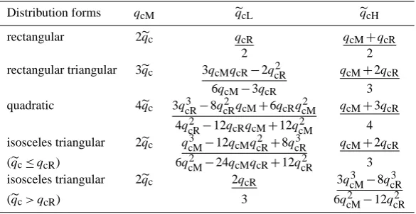
Table 2. Maximum values of CWC (qcM) and local mean values of CWC in low (eqcL) and high (eqcH) CWC regions for four different CWC PDF forms. The threshold value allowing precipitation formation is identified withqcR.
Distribution forms qcM eqcL eqcH
rectangular 2eqc qcR qcM+qcR
2 2
rectangular triangular 3eqc 3qcMqcR−2q 2
cR qcM+2qcR 6qcM−3qcR 3 quadratic 4eqc 3q
3
cR−8qcR2 qcM+6qcRqcM2 qcM+3qcR 4qcR2 −12qcRqcM+12qcM2 4 isosceles triangular 2eqc q
3
cM−12qcMqcR2 +8qcR3 qcM+2qcR (eqc≤qcR) 6q
2
cM−24qcMqcR+12qcR2 3 isosceles triangular 2eqc 2qcR 3q
3 cM−8qcR3
(eqc> qcR) 3 6q
2
cM−12qcR2
functions could be suitable for describing its PDF (as it will be shown later in Fig. 12). To evaluate the sensitivity of the scheme to the PDF choice, tests were extended to rectangu-lar and two triangurectangu-lar PDF, as shown by Fig. 1. A variable namedqcMwas added as the limit for the integration of the CWC and it is derived from the conservation of the CWC in the grid box. Figure 1 shows all four PDF with the low (light grey) and high (dark grey) CWC regions forq˜c< qcR(left column) andq˜c> qcR (right column). Table 2 shows how parameters of the distribution were derived from the mean CWC value in the cloud fraction. Figure 2 shows howqcM,
˜
qcLandq˜cH increased with increasing values ofq˜c. In fact, the different PDF shapes did not significantly affect the rela-tionship between the mean CWC value in the cloud fraction and the mean of the values higher than the collection thresh-old that drove the autoconversion rate. As soon as the CWC is split into a high and a low part,q˜cH>q˜c, but there is lit-tle difference between theq˜cHvalues derived using the four different PDF forms.
3.3 Rain fraction
The local value of rain water content (RWC) was defined, like the local value of cloud water, asq˜r= ¯qr/RF, where RF is the rain fraction in the model grid. The rain fraction, how-ever, could not be diagnosed like the cloud fraction because rain drops fall to the ground. The challenge was to address this probabilistic issue without adding more prognostic vari-ables into the model.
When precipitation forms in a model grid void of precip-itating drops, the solution is straightforward since it is con-fined to the grid fraction whereq˜cHbecomes greater than the collection threshold and RF is initially set to CFH.
A realistic approach would be to advect the rain fraction like any conservative variable, considering that the fraction is uniformly distributed over each model grid. This is feasi-ble if one more prognostic variafeasi-ble is added, namely the sub-grid value of the RWC. After advection, the rain fraction can thus be calculated asq˜r/q¯r. At this stage, however, a simpler, economical solution was tested that did not require an addi-tional variable. The RWC is advected like all other model variables and the rain fraction is following the rain in the column: once precipitation had formed in a model column,
�
qc< qcR �qc> qcR
a1 Rectangular PDF a2
b1 Rectangular triangular PDF b2
c1 Quadratic PDF c2
d1 Isosceles triangular PDF d2
Figure 1: Graphs of the four PDF forms used to represent the CWC. Light grey represents regions of low CWC and dark grey represents high CWC. The local mean CWC, the local low CWC and local high CWC are, respectively,�qc,�qcLand�qcH. The autoconversion threshold isqcR, and the maximum value of the CWC isqcM.
25
Fig. 1. Graphs of the four PDF forms used to represent the CWC. Light grey represents regions of low CWC and dark grey represents high CWC. The local mean CWC, the local low CWC and local high CWC are, respectively,eqc,eqcLandeqcH. The autoconversion threshold is qcR, and the maximum value of the CWC isqcM.
the rain fraction was translated to the whole column below, down to the ground. In other words, the rain fraction in a model column was equal to the maximum of the rain frac-tions at the levels where rain is formed. Note that there is no horizontal advection of the rain fraction. Because RWC can be advected but its fractional part cannot, possible incon-sistencies between this simple probabilistic approach and the 3-D advection of RWC were further accounted for by setting
the rain fraction to zero in grids where the RWC was less than a small threshold value.
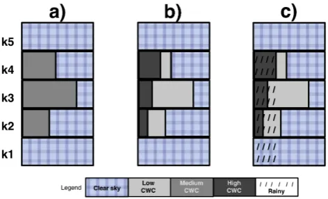
3.4 Vertical overlap
Vertical overlap of clouds and rain fractional areas is also a probabilistic issue. In order to maximize precipitation for-mation for cumulus and stratocumulus clouds, the maximum cloud overlap assumption was used for CF and RF in the new parameterization (see Fig. 3).
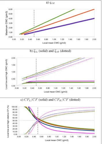
a)
qcM
b)
q
�
cL(solid) and
�
q
cH(dotted)
c)
CFL/CF
(solid) and
CFH
/CF
(dotted)
Figure 2: Variations of (a) the maximum CWC (
qcM
), (b) the mean local low (
qcL
�
, solid lines) and high
(�
qcH
, dotted lines) CWC and (c) the relative cloud fractions in low CWC region (solid lines) and high
regions (dotted lines) as a function of
q
�
c. The four PDF forms are rectangular (blue), rectangular
trian-gular (red), quadratic (green) and isosceles triantrian-gular (pink). A vertical dashed grey line is added at the
autoconversion threshold. Note that two grey reference lines are added in Fig. b and c, and the blue line
is overlapping the pink one in Fig. a.
26
Fig. 2. Variations of (a) the maximum CWC (qcM), (b) the mean local low (eqcL, solid lines) and high (eqcH, dotted lines) CWC and (c) the relative cloud fractions in low CWC region (solid lines) and high regions (dotted lines) as a function ofeqc. The four PDF forms are rectangular (blue), rectangular triangular (red), quadratic (green) and isosceles triangular (pink). A vertical dashed grey line is added at the autoconversion threshold. Note that two grey reference lines are added in (b) and (c), and the blue line is overlapping the pink one in (a) .
Following the same concept, it was assumed that the rain fraction sedimented preferentially in the cloud core (CFH). If RF>CFH, the remainder rainwater fell from the diluted cloud fraction CFL and if RF>CF, the remaining rainwater
fell through clear air. Such an assumption mimics the LES when clouds are growing vertically, but it obviously fails for multi-layered clouds or when clouds are tilted because of wind shear.
Figure 3: The three columns are the successive steps of the numerical treatment of the cloud and rain vertical overlap in a model column. (a) The maximum cloud overlap is applied for adjacent or non-adjacent layers. (b) The same maximum cloud overlap of (A) is applied for the new parameterization using the splitting of the CWC in two regions, and maximally overlapping the high CWC regions. (c) The rain is falling vertically with a maximum vertical overlap.
27
Fig. 3. The three columns are the successive steps of the numerical treatment of the cloud and rain vertical overlap in a model column with 5 levels: k1, k2, k3, k4, and k5. (a) The maximum cloud over-lap is applied for adjacent or non-adjacent layers. (b) The same maximum cloud overlap of (a) is applied for the new parameteriza-tion using the splitting of the CWC in two regions, and maximally overlapping the high CWC regions. (c) The rain is falling vertically with a maximum vertical overlap.
Figure 4: Four horizontal views of a grid box, with the splitting of the CWC in two regions of low and high CWC. RF and CF are the rain and the cloud fractions, withCFLrepresenting the cloud fraction
in the low CWC region andCFHthe cloud fraction in the high CWC region (see text for details about
differences in accretion and rain evaporation in a, b, c and d).
28
Fig. 4. Four horizontal views of a grid box, with the splitting of the CWC in two regions of low and high CWC. RF and CF are the rain and the cloud fractions, with CFLrepresenting the cloud fraction in the low CWC region and CFHthe cloud fraction in the high CWC region (see text for details about differences in accretion and rain evaporation in a, b, c and d).
3.5 Accretion and drop evaporation
Following the above assumption, the ways drops collect droplets in the area where rain fraction overlaps cloud frac-tion or evaporate when the rain fracfrac-tion overlaps with clear air depend on the respective values of RF, CF, CFHand CFL:
Table 3. List of C-130 flights for DYCOMS-II used in this study. Drizzle rates are from van Zanten et al. (2005).
Flight number Date Flight condition Drizzle rate (mm day−1)
RF01 20010710 night none
RF02 20010711 night 0.35±0.11 RF03 20010713 night 0.05±0.03 RF04 20010717 night 0.08±0.06
RF05 20010718 night none
RF07 20010724 night 0.60±0.18
RF08 20010725 day 0.12±0.03
a. RF = CFH: accretion is calculated usingq˜cH and there is no evaporation (see Fig. 4a).
b. CFH<RF<CF: accretion is calculated usingq˜cHin the CFH region andq˜cLin the RF−CFH region, and there is no evaporation (see Fig. 4b).
c. CF<RF: accretion is calculated as above and evapora-tion occurs in the remaining rain fracevapora-tion RF−CF (see Fig. 4c).
d. CFH= 0: accretion is calculated using q˜c and q˜r in the overlapping part of CF and RF, and evaporation is calculated if RF>CF (see Fig. 4d).
4 DYCOMS-II stratocumulus case
The DYCOMS-II campaign (Stevens et al., 2003) took place near the coast of California in 2001 to document noctur-nal stratocumulus layers over the ocean. The data were collected on board the NCAR-C130 instrumented aircraft, equipped more specifically for in-situ cloud microphysics with the King Probe and PVM-100, a comprehensive suite of optical particle spectrometers (SPP-100, FOAP-260X and OAP-2DC), and the radar from the University of Wyoming (94 GHz) for remote sensing of drizzle particles. The data set included 6 nocturnal case studies and one daytime flight (see Table 3).
Flight RF02 of the DYCOMS-II campaign was selected to develop an idealized case of marine nocturnal stratocumu-lus for the intercomparison of 11 LES models (Ackerman et al., 2009). LES were run with both the single and double moment schemes, with low CCN concentrations correspond-ing to the typical values measured durcorrespond-ing the campaign (van Zanten et al., 2005).
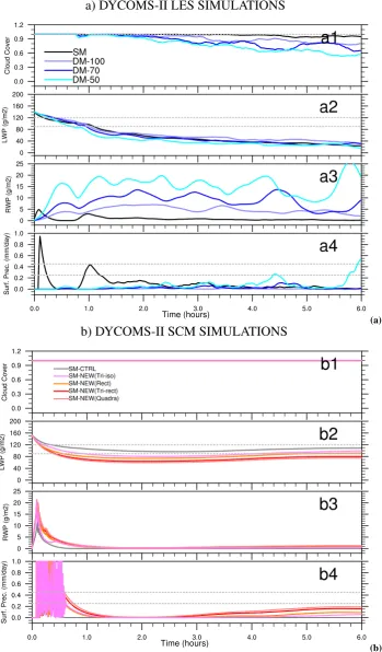
a) DYCOMS-II LES SIMULATIONS
b) DYCOMS-II SCM SIMULATIONS
Figure 5: Mean temporal evolution over the entire domain for DYCOMS-II LES (a) and SCM (b)
sim-ulations. From top to bottom: cloud cover, integrated cloud water content (LWP,
g
/
m
2) and rain water
content (RWP,
g
/
m
2) and surface precipitation (Surf. Prec.,
mm
/
day
).
29
(a)
a) DYCOMS-II LES SIMULATIONS
b) DYCOMS-II SCM SIMULATIONS
Figure 5: Mean temporal evolution over the entire domain for DYCOMS-II LES (a) and SCM (b)
sim-ulations. From top to bottom: cloud cover, integrated cloud water content (LWP,
g
/
m
2) and rain water
content (RWP,
g
/
m
2) and surface precipitation (Surf. Prec.,
mm
/
day
).
29
(b)
Fig. 5. Mean temporal evolution over the entire domain for DYCOMS-II LES (a) and SCM (b) simulations. From top to bottom: cloud cover, integrated cloud water content (LWP, g m−1) and rain water content (RWP, g m−1) and surface precipitation (Surf. Prec., mm day−1).
DYCOMS-II LES SIMULATIONS
a) SM b) DM-50
DYCOMS-II SCM SIMULATIONS
c) SM-CRTL d) SM-NEW
Figure 6: Vertical profiles of cloud fraction (CF), cloud water content (�qc), rain fraction (RF) and rain
water content (�qr) for LES and SCM simulations of DYCOMS-II. Mean values from observation are
added with black dots and standard deviation with black lines.
30
Fig. 6. Vertical profiles of cloud fraction (CF), cloud water content (eqc), rain fraction (RF) and rain water content (eqr) for LES and SCM simulations of DYCOMS-II. Mean values from observation are added with black dots and standard deviation with black lines.
4.1 LES results of DYCOMS-II
Figure 5a summarizes the results of the 4 simulations (DM-50, DM-70, DM-100 and SM), with dashed grey lines for the observed values of cloud cover, LWP (Liquid Water Path) and surface precipitation rate from van Zanten et al. (2005). After slightly less than one hour of spin-up, the simulations develop a stratocumulus layer with cloud cover and an LWP comparable to those observed. The simulations do not reach equilibrium, however, and all cloud parameters progressively collapse, as was the case for some of the models participat-ing in the intercomparison (van Zanten et al., 2005) and in the work of Geoffroy et al. (2008) for the same case. Six hours into the simulation, the LWP reaches a value less than one third of the observed one. The precipitation rate at the surface is also much lower than observed, except for the
DM-50 simulation, which exhibits two short periods (at 4 h 30 and 6 h) of enhanced precipitation reaching the observed val-ues, but overall the precipitation rates remain very small for all LES simulations compared to observations (see Table 4). Take note that the precipitation rates presented in Table 4 are cumulated over the last 4 h to avoid artifacts of the initial spin-up period.
During RF02, the cloud fraction was close to 100 %, a value well reproduced by the SM simulation. The DM simu-lations, in contrast, gave cloud fractions lower than unity, de-creasing to 60 % for the DM-50 simulation. With such a low cloud fraction, the LWP could reach local values more than double the mean, which explains why the DM-50 simulation produced higher precipitation rates at the surface despite its low mean LWP.
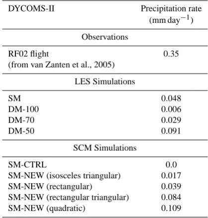
Table 4. Observed and simulated surface precipitation rates for DYCOMS-II.
DYCOMS-II Precipitation rate
(mm day−1)
Observations
RF02 flight 0.35
(from van Zanten et al., 2005)
LES Simulations SM 0.048 DM-100 0.006 DM-70 0.029 DM-50 0.091 SCM Simulations SM-CTRL 0.0
SM-NEW (isosceles triangular) 0.017 SM-NEW (rectangular) 0.039 SM-NEW (rectangular triangular) 0.084
SM-NEW (quadratic) 0.109
Direct comparisons of observed and simulated LWP and RWP (Rain Water Path) are more problematic because they require vertical integration of values measured along hori-zontal flight legs. The vertical profiles of CWC and RWC, though, provide valuable information for the qualification of the simulations. Figure 6a and b showsq˜candq˜rvertical pro-files, with their respective fractions. The observed values are represented by black dots (mean) and black lines (standard deviation), and colored lines represent the mean simulated fields for each hour. The simulated profiles ofq˜c are simi-lar to the observed ones, with a quasi-adiabatic increase with height above cloud base. Forq˜r profiles, the SM ones are lower than the observed ones and the opposite for the DM-50 ones.
This simulation, however, does not reach quasi-equilibrium and the simulated LWP decreases with time. Af-ter one hour of simulation, cloud base height continuously increases while the top altitude remains constant. The cloud layer gets thinner and LWP decreases. With the SM scheme, the cloud fraction remains close to unity, the LWP is uni-formly distributed and thus becomes too small for drizzle to form. With the DM scheme, the cloud fraction decreases so that local values of the LWP remain sufficient for autoconver-sion to temporarily produce rainwater and precipitation rates similar to the observed ones.
4.2 Microphysics statistics for DYCOMS-II
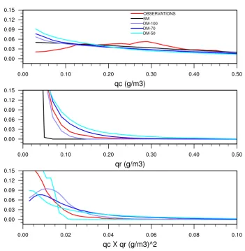
Rain water content is a highly variable parameter with an ex-ponentially decreasing frequency distribution that results in its mean value being insufficient to describe its statistical dis-tribution. Comparison with the observed frequency distribu-tions thus provides a more robust qualification for LES. Fig-ure 7 shows the frequency distributions ofqc,qrandqc×qr from the observations, and the 4 LES simulations. The prod-uct of CWC by RWC is an interesting parameter because ac-cretion, which generates most of the precipitating particles, is proportional to this product. There is good agreement be-tween the LES and observations forqr, but it can be seen that, for qc, the model overestimates the frequency of the small values. From DYCOMS-II CWC observations, the isosceles triangular PDF form is more appropriate, as was also shown in the ACE-2 stratocumulus case (Brenguier et al., 2003).
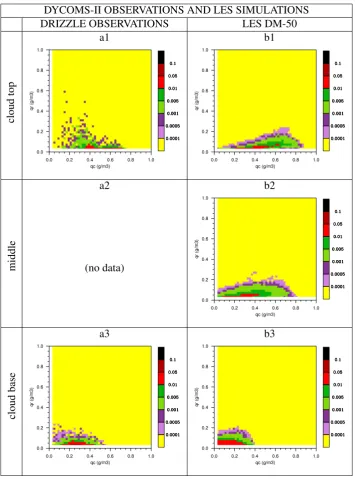
Realistic simulations of the qc, qr and qc×qr fields are crucial for NWP models, in which the collection process of droplet growth into precipitating drops is reduced to a two-stage bulk parameterization with power laws ofqcfor auto-conversion and ofqc×qrfor accretion. Figure 8 shows the joint frequency distributions ofqc andqr, as observed and simulated in the DM-50 simulation. Statistics are stratified in three levels, from cloud base to the cloud top. The fig-ure supplements the above analysis of the vertical profiles where the LES model produces largeqc values, much more frequently close to cloud top than observed. More interest-ing is the fact that the largestqrvalues in the DM-50 case are concomitant with the largestqcvalues at cloud top, while ob-servations show the opposite, with largeqcat smallqrvalues and vice versa.
4.3 SCM results of DYCOMS-II
Figure 5b shows the SCM results as in Fig. 5a for LES sim-ulations. The cloud cover is 100 % as in the observations and the LWP follows what was observed at the end of the simulation after a slight decrease below the observed value. The surface precipitation rates stabilize after 5 h to a constant value just below the minimum observed value.
Figure 6c and d show the vertical profiles of CF, RF,q˜cand
˜
qr using the standard scheme (SM-CTRL) and the profiles obtained with the subgrid precipitation scheme (SM-NEW, rectangular triangular PDF of CWC). In both cases the cloud fraction is 100 % and the CWC profiles are similar to ob-served and LES values as shown in Fig. 6a and b. The stan-dard scheme, however, does not generate any precipitation because the peak values remain smaller than the collection threshold (0.5 gm−3). In contrast, the subgrid scheme pro-duces values greater than 1.5 gm−3over a rain fraction that covers the whole domain. The rain sedimentation scheme rapidly distributes the rainwater over the whole grid and the rain fraction remains at 100 % for the duration of the simula-tion.
DYCOMS-II OBSERVATIONS AND LES SIMULATIONS
Figure 7: Relative frequency distributions of
q
c,
q
rand
q
c×
q
rfor observations and LES simulations of
DYCOMS-II.
31
Fig. 7. Relative frequency distributions ofqc,qrandqc×qrfor observations and LES simulations of DYCOMS-II.
4.4 Validation of the cloud water splitting for DYCOMS-II
Figure 9a shows how cloud water is distributed within the observed cloud with the vertical profiles ofq˜c(black dots),
˜
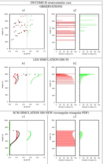
qcL(red dots) andq˜cH(green dots). The right panel shows the fraction of samples used to calculate mean values. Figure 9b is similar for the LES using the DM-50 scheme after 5 h of simulation and Fig. 9c shows the fractions diagnosed with the subgrid precipitation scheme (triangular PDF of CWC) after 5 h of simulation. The comparison illustrates how the sub-grid scheme develops between 10 and 20 % of the CWC val-ues greater than the collection threshold, in agreement with the LES, and hence generates noticeable values of rain water mixing ratio.
5 RICO cumulus case
The RICO field experiment (Rauber et al., 2007) took place in the Caribbean in the vicinity of Antigua Island during the winter of 2004–2005 to document fair weather cumuli over the ocean. The data were collected onboard the NCAR-C130, with the same microphysics instrumentation used dur-ing DYCOMS-II, and the University of Wyomdur-ing radar. The data set includes 19 flights (see Table 5). The observed cloud cover was less than 10 % (0.086 from Zhao and Di Girolamo, 2007) and the mean precipitation rate was 2.23 mm day−1, with values between 0 and 22 mm day−1(from Snodgrass et al., 2008).
5.1 LES results of RICO
Based on the period of 16 December 2004 to 8 January 2005, van Zanten et al. (2011) defined a composite case for model intercomparison. This period corresponded to fair weather cumuli generating a mean precipitation rate of 0.3 mm day−1. More details on the initialization fields and
DYCOMS-II OBSERVATIONS AND LES SIMULATIONS
DRIZZLE OBSERVATIONS
LES DM-50
a1
b1
cloud
top
a2
b2
middle
(no data)
a3
b3
cloud
base
Figure 8: Joint probability distribution of
q
cand
q
rfor cloud top, middle part and cloud base using
DYCOMS-II observations and LES simulation DM-50.
32
Fig. 8. Joint probability distribution ofqc and qr for cloud top, middle part and cloud base using DYCOMS-II observations and LES simulation DM-50.
large-scale forcings are available at www.knmi.nl/samenw/ rico/setup3d.html. As for the stratocumulus case, Meso-NH simulations were performed with both the SM and DM schemes, the latter with low CCN concentrations correspond-ing to the typical values measured durcorrespond-ing the campaign (Hud-son and Mishra, 2007).
Figure 10a summarizes the results of the 4 simula-tions. After 2 h of model spin-up, the SM simulation reaches pseudo-equilibrium with cloud cover of 10 %, LWP
of 10 gm−2, RWP of 3 gm−2 and a surface rain rate of 0.2 mm day−1. The DM simulations, in contrast, exhibit a continuous increase of the cloud fraction, reaching a cloud fraction of 20 % after 24 h, while the liquid and rainwater paths are comparable to the SM simulation. The precipi-tation rate using the DM scheme increases with decreasing CCN concentrations (see Table 6). Overall, these simula-tions generate precipitation rates comparable to the average rates over the period of observation.
DYCOMS-II stratocumulus case OBSERVATIONS
a1 a2
LES SIMULATION DM-50
b1 b2
SCM SIMULATION SM-NEW (rectangular triangular PDF)
c1 c2
Figure 9: (Left) Mean values of total CWC (q�c, black dots), mean CWC in the low CWC region (q�cL, red
dots) and in the high CWC region (q�cH, green dots). (Right) Number of data (percent) used to calculate
the corresponding mean values at the left.
33
Fig. 9. (Left) Mean values of total CWC (eqc, black dots), mean CWC in the low CWC region (eqcL, red dots) and in the high CWC region (eqcH, green dots). (Right) Number of data (percent) used to calculate the corresponding mean values at the left.
As in the model intercomparison test, our LES (Fig. 11a and b) shows reasonable agreement with the observed CWC vertical profile (see Fig. 8 in van Zanten et al., 2011), and the same tendency to overestimateq˜c when approaching cloud top. The vertical profiles of q˜r also agree, at least for the
order of magnitude around 0.1 gm−3, although the simulated values increase slightly with altitude above cloud base, while the observations show no particular trend.
There is good agreement between LES and observations for the frequency distributions ofqc,qr, andqc×qr(Fig. 12),
512 S. Turner et al.: A subgrid parameterization scheme for precipitation
a) RICO LES SIMULATIONS
b) RICO SCM SIMULATIONS
Figure 10: Same as Fig. 5 for RICO.
34
14
S. Turner et al.: A subgrid parameterization scheme for precipitation
a) RICO LES SIMULATIONS
b) RICO SCM SIMULATIONS
Figure 10: Same as Fig. 5 for RICO.
34
Fig. 10. Same as Fig. 5 for RICO.
but it can be observed that the model is reproducing drizzle
(low
q
rvalues more frequent) instead of rain, as was
sug-gested by van Zanten et al. (2011), with precipitation
occur-ring too frequently (and too lightly) in most of the models of
the intercomparison study.
Finally the joint frequency distributions at cloud top show
that the largest
q
rvalues in the DM LES are concomitant with
the largest
q
cvalues, while observations show the opposite,
with large
q
cat small
q
rand vice versa (Fig. 13). This feature
is more noticeable near cloud top.
Geosci. Model Dev., 5, 1–22, 2012
www.geosci-model-dev.net/5/1/2012/
Fig. 10. Same as Fig. 5 for RICO.
but it can be observed that the model is reproducing drizzle (lowqr values more frequent) instead of rain, as was sug-gested by van Zanten et al. (2011), with precipitation occur-ring too frequently (and too lightly) in most of the models of the intercomparison study.
Finally the joint frequency distributions at cloud top show that the largestqrvalues in the DM LES are concomitant with the largestqc values, while observations show the opposite, with largeqcat smallqrand vice versa (Fig. 13). This feature is more noticeable near cloud top.
RICO LES SIMULATIONS
a) SM b) DM-50
RICO SCM SIMULATIONS
c) SM-CRTL d) SM-NEW
Figure 11: Same as Fig. 6 for RICO.
35
Fig. 11. Same as Fig. 6 for RICO.
5.2 SCM results of Rico
Figure 10b is similar to Fig. 10a for the SCM results, and a test simulation has been added following Bechtold et al. (1993) (named SM-TESTB93). The main difference be-tween this last test and all other simulations is that the cloud water is uniformly distributed in the cloud fraction and the rain fraction is defined to be the same as the cloud fraction. There is then no splitting of the cloud water in two regions and it takes a longer time to produce rain since the whole cloud fraction must reach the threshold value to produce rain. Despite the fact that the SM-CTRL run has a similar cloud cover and a higher LWP, it is not able to produce surface rain at all. The four SM-NEW runs produce similar cloud cover, LWP and RWP, reaching a constant precipitation rate after 16 h. The SM-TESTB93 run produces more precipita-tion than the CTRL, but slightly less than the four SM-NEW runs. The cumulative precipitation rates for 24 h are compared in Table 6.
Figure 11c and d are similar to Fig. 11a and b for the SCM results. The cloud fraction decreases sharply with altitude above cloud base but, within this small fraction, the CWC follows a quasi-adiabatic profile. Both the standard and the subgrid precipitation schemes generate significant values of
˜
qc, greater than the autoconversion threshold over most of the cloud depth. This feature is intrinsic to the subgrid con-vection scheme, which predicts a realistic grid CWC mean value but distributes it over a cloud fraction that is too small, thus overestimatingq˜c. However, the standard scheme was not able to produce rain while the new scheme is generating rain of the order of the observed one.
The difference between the original and the new schemes is the distribution of the rain water content produced, which is spread over the whole grid in the standard scheme while it is confined to a column corresponding to the cloud fraction in the subgrid scheme. This difference explains why the surface precipitation rate is higher within the subgrid scheme while most of the rain particles evaporate when they are spread over the whole grid in the original formulation.
RICO OBSERVATIONS AND LES SIMULATIONS
Figure 12: Same as Fig. 7 for RICO.
36 Fig. 12. Same as Fig. 7 for RICO.
Table 5. List of C-130 flights for RICO used in this study. Rain rates (RR) are from Snodgrass et al. (2009).
Flight number Date Rain Rate (mm day−1)
RF01 20041207 0<RR<1 RF02 20041208 1<RR<2 RF03 20041209 1<RR<2 RF04 20041210 1<RR<2 RF05 20041213 17<RR<18
Beginning of the LES composite period
RF06 20041216 3<RR<4 RF07 20041217 0<RR<1 RF08 20041219 2<RR<3 RF09 20041220 0<RR<1 RF10 20050105 1<RR<2 RF11 20050107 0<RR<1
End of the LES composite period
RF12 20050111 1<RR<2 RF13 20050112 1<RR<2 RF14 20050114 2<RR<3 RF15 20050116 1<RR<2 RF16 20050118 3<RR<4 RF17 20050119 1<RR<2 RF18 20050123 0<RR<1 RF19 20050124 0<RR<1
Table 6. Observed and simulated surface precipitation rates for RICO.
RICO Precipitation rate
(mm day−1)
Observations
Three weeks composite 0.3 (mean) (Nuijens et al., 2005)
Two months 2.23 (mean)
(Snodgrass et al., 2008) 0 to 22 (extremes)
LES Simulations
SM 0.099
DM-100 0.327
DM-70 0.429
DM-50 0.528
SCM Simulations
SM-CTRL 0.007
SM-NEW (isosceles triangular) 0.409
SM-NEW (rectangular) 0.451
SM-NEW (rectangular triangular) 0.469
SM-NEW (quadratic) 0.479
SM-TESTB93 0.299
5.3 Validation of the cloud water splitting for RICO
A representation similar to the higher and lower CWC for the stratocumulus case was made for the cumulus case (see Fig. 14). The SM-NEW simulation producesq˜cL similar to the DM-50 and observations, butq˜cH is too high from the cloud middle to top. The fractional area of higher CWC val-ues is too high (>20 %) in both LES and SCM simulations compared to the low values (<20 %) of the observational data sets.
In summary, these two idealized cases (stratocumulus and cumulus) illustrate important features of the subgrid scheme. On the one hand, the scheme allows for generation of pre-cipitation in grids where rain production is not activated with the standard scheme because the mean cloud water mixing ratio is smaller than the collection threshold. On the other hand, it shows how important the distribution of the CWC is to produce rainwater in the grid when the cloud fraction is very small, as in the RICO case.
6 Real test case
The real case of 27 March 2009 with precipitating BL clouds was chosen to test the subgrid precipitation scheme. Due to a surface trough located between Scotland and Norway, westerly flow was established over France, bringing moist air into the southwestern part of France. The associated BL
RICO OBSERVATIONS AND LES SIMULATIONS
RAIN + DRIZZLE OBS. LES SM LES DM-50
a1 b1 c1
cloud
top
a2 b2 c2
middle
a3 b3 c3
cloud
base
Figure 13: Same as Fig. 8 for RICO.
37
Fig. 13. Same as Fig. 8 for RICO.
clouds produced drizzle with low precipitation rates leading to cumulative precipitation of around 1 mm at the ground be-tween 00:00 and 06:00 UTC (Fig. 15a). The AROME op-erational model simulated the BL clouds correctly but did not reproduce the associated drizzle (Fig. 15b). The Meso-NH model, in the same configuration (2.5 km horizontal res-olution, 60 vertical levels) with the same physics (ICE3 mi-crophysics, turbulence and shallow convection scheme), pro-duced similar cloud coverage over the continent and also failed to reproduce the observed drizzle (Fig. 15d).
The activation of the subgrid precipitation scheme cor-rected the lack of precipitation, allowing the model to pro-duce small amounts of rain continuously during the 6-h period, although these predictions (between 0.2 mm and 1 mm) slightly underestimated the amount of rain seen in the observations (Fig. 15c). A vertical cross section at 06:00 UTC from south to north for the two Meso-NH simula-tions (Fig. 16) shows the drizzle associated with stratocumu-lus coverage, and also rain production of the deeper cumustratocumu-lus clouds in the northern part of the domain, giving a more con-tinuous rain transition between stratocumulus and deeper
cu-mulus clouds. The rain significantly modifies the predicted cloud water content, leading to generally lower values due to the collection processes.
Other real-case tests with non-precipitating BL clouds were conducted to check that the subgrid precipitation scheme did not produce rain systematically since theq˜cvalue must be greater thanqcMto initiate cloud water splitting.
7 Conclusions
In summary, two cloud types were considered in this study, stratocumulus sampled over the northeastern Pacific during DYCOMS-II and a field of fair weather cumuli sampled in the Caribbean during RICO. Model intercomparison exer-cises have been performed recently, one based on a single DYCOMS-II case study (RF02), the other using a composite case based on 24 days of the RICO campaign. We used these initialization and forcing fields to perform LES simulations configured with cloud microphysics parameterization using either a single moment scheme or a double moment scheme with three different values of CCN concentrations. The LES
RICO cumulus case OBSERVATIONS
a1 a2
LES SIMULATION DM-50
b1 b2
SCM SIMULATION SM-NEW (rectangular triangular PDF)
c1 c2
Figure 14: Same as Fig. 9 for RICO.
38
Fig. 14. Same as Fig. 9 for RICO.
produced realistic precipitation rates at the surface for the cumulus case, but underestimated them for the stratocumu-lus case. The cloud macrophysical properties, however, were not necessarily in full agreement with the observations, espe-cially for the DYCOMS-II case, for which the LES was
un-able to reach equilibrium. Moreover, the statistical distribu-tions of cloud and precipitating water were also slightly dif-ferent between models and observations, suggesting that the autoconversion scheme is not as efficient as the actual col-lection process. The similar results between the observations
CUMULATIVE PRECIPITATION BETWEEN 00 AND 06 UTC (mm)
a) OBSERVATIONS b) AROME
c) 3D-NEW MESO-NH d) 3D-CTRL MESO-NH
Figure 15: Cumulated precipitation between 00 and 06 UTC in South-West France for March 27, 2009.
39
Fig. 15. Cumulated precipitation between 00:00 and 06:00 UTC in South-West France for 27 March 2009.
and the LES simulations are considered sufficient for the LES fields to be used to extend the limited statistics derived from the observations.
For the stratocumulus case, drizzle within the clouds was easily reproduced with LES simulations, but it evaporated almost completely before reaching the ground. The SCM simulations with the new parameterization using one of the four CWC PDFs were all able to produce drizzle reaching the ground, but with a lower value than the observed one. This is better than the original formulation, which was not able to produce surface drizzle at all.
Regarding the cumulus cloud case, the new subgrid param-eterization greatly enhanced precipitation rates by allowing a smaller rain fraction within the cloud fraction and reducing evaporation during the sedimentation process.
A real case of precipitating stratocumulus over France demonstrated the potential of the proposed subgrid
param-eterization by producing a small rain area that was missed completely by the operational model.
Hence, the parameterization improves warm microphysics by smoothing the transition from non-precipitating to fully precipitating model grids. It is, however, sensitive to the subgrid condensation scheme that provides the diagnosis of cloud fraction and of the local CWC values. The cumulus case study, for instance, reveals that the convective scheme of Pergaud et al. (2009) produces high (almost adiabatic) CWC values over a cloud fraction that is too small. Conse-quently, the subgrid precipitation scheme produces too much rain within a cloud fraction that is too small, and results in values that were not observed during previous field cam-paigns. The scheme is now being tested against real cases of different meteorological situations to establish the poten-tial of the new parameterization and to detect weaknesses.
3D-CTRL MESO-NH 3D-NEW MESO-NH a)r¯c( g/kg) b)¯rc( g/kg)
c)r¯r( g/kg) d)r¯r( g/kg)
e)r¯c( g/kg)at 800 m f)r¯c( g/kg)at 800 m
Figure 16: Cross section ofr¯c(a and b) andr¯r(c and d) for Meso-NH runs 3D-CTRL (left) and 3D-NEW
(right). (e and f) Mean cloud water content at 800 m for 06 UTC March 27, 2009, with the cross section indicated by the black line.
40
Fig. 16. Cross section ofr¯c(a and b) andr¯r(c and d) for Meso-NH runs 3-D-CTRL (left) and 3-D-NEW (right). (e and f) Mean cloud water content at 800 m for 06:00 UTC, 27 March 2009 with the cross section indicated by the black line.
Appendix A
ICE3 warm processes formulation
According to the ICE3 microphysics scheme (Pinty and Jabouille, 1998), the following are the equations for au-toconversion, accretion, evaporation and sedimentation of rain in the warm part of the scheme. All equations are given in terms of the mixing ratios of water vapor, cloud and rain water, respectively, rv, rc and rr (with
units of kg kg−1). More information is available online
in the scientific documentation of the Meso-NH model (http://mesonh.aero.obs-mip.fr/mesonh/).
Autoconversion in the ICE3 scheme is a Kessler type
formu-lation:
∂rr
∂t
autoconv
=kcrit×MAX(0,rc−rc crit) (A1) wherekcrit=10−3s−1, rc crit=qc crit/ρd, ρd is the dry air
density andqccrit=0.5×10⁻³kg m−3.
Accretion in the ICE3 scheme is of the form: ∂rr ∂t accr =π 4cNor
ρo
ρd 0.4
0(d+3)
ρd
πρwNor
(d+3)/4
rcr(d +3)/4
r (A2)
wherec=842 m s−1, d=0.8, ρw is the moist air density,
ρo is the air density at the reference pressure level, and
Nor=8.0×10⁶m−3is set constant.
Evaporation in the ICE3 scheme is of the form:
∂rr
∂t
evap (A3)
= −2π SNor Aρd
"
¯ f1
ρdrr
πρwNor 1/2
+ ¯f2 ρo ρd 0.4/2 c νcin 1/2
0(d+5
2 )
ρdrr
πρwNor (d+5)/8#
wheref¯1=1 andf¯2=0.22 are ventilation coefficients,νcin is the air kinematic viscosity, which is here assumed to be constant νcin=0.15×10⁻⁴kgm−1s−1. The function S is given by:
S=1− rv
rvs
(A4) wherervsis the saturated vapor mixing ratio. The thermody-namic function A is:
A' RvT
es(T )Dv
+(Lv(T ))
2
kaRvT2
(A5) whereT is the temperature, Rv=461.51Jkg−1K−1, Dv=
2.26×10⁻⁵ms−1is the diffusivity of water vapor in air and
ka=24.3×10⁻³Jm−1s−1K−1is the heat conductivity of air.
(for simplicity,Dvandkaare taken constants). es(T )is the
saturation vapor pressure and is computed according to
es(T )=exp αw−
βw
T −γwln(T )
(A6) using
αw =ln(es(T0))+ βw
T0
−γwln(T0) (A7)
βw =
Lv(T0) Rv
γwT0 (A8)
γw =
Cl−Cpv
Rv
(A9) whereT0=273.16K andLvis the latent heat of vaporization
and is computed according to:
Lv(T )=Lv(T0)+(Cpv−Cl)(T−T0) (A10) whereCpv=1850Jkg−1K−1,Lv(T0)=2.5×10⁶Jkg−1 and Cl=4.218×10³.
Sedimentation rate in the ICE3 scheme is of the form:
∂rr
∂t sed=
cρ0.4o 6ρd
0(d+4) [πρwNor]d/4
∂ ∂z
h
(ρd)1+d/4−0.4(rr)1+d/4
i (A11)
Acknowledgements. This work was partly funded by GAME/CNRM (M´et´eo-France, CNRS) and EUCAARI (Eu-ropean Integrated project on Aerosol Cloud Climate and Air Quality interactions) No 036833-2. Discussions through the COST Action ES0905 are acknowledged.
Edited by: A. Lauer
The publication of this article is financed by CNRS-INSU.
References
Ackerman, A. S., van Zanten, M. C., Stevens, B., Savic-Jovcic, V., Bretherton, C. S., Chlond, A., Golaz, J.-C., Jiang, H., Khairout-dinov, M., Krueger, S. K., Lewellen, D. C., Lock, A., Moeng, C.-H., Nakamura, K., Petters, M. D., Snider, J. R., Weinbrecht, S., and Zulauf, M.: Large-Eddy Simulations of a Drizzling, Stratocumulus-Topped Marine Boundary Layer, Mon. Weather Rev., 137, 3, 1083–1110, 2009.
Arakawa, A.: The Cumulus Parameterization Problem: Past, Present, and Future, J. Climate, 17, 13, 2493–2525, 2004. Barrett, A. I., Hogan, R. J., and O’Connor, E. J.: Evaluating
fore-casts of the evolution of the cloudy boundary layer using diurnal composites of radar and lidar observations, Geophys. Res. Lett., 36, L17811, doi:10.1029/2009GL038919, 2009.
Bechtold, P., Pinty, J.-P., and Mascart, P.: The Use of Partial Cloudi-ness in a Warm-Rain Parameterization: A Subgrid-Scale Precip-itation Scheme, Mon. Weather Rev., 121, 12, 3301–3311, 1993. Bechtold, P., Cuijpers, J. W. M., Mascart, P., and Trouilhet, P.:
Modeling of Trade Wind Cumuli with a Low-Order Turbulence Model: Toward a Unified Description of Cu and Se Clouds in Meteorological Models, J. Atmos. Sci., 52, 4, 455–463, 1995. Berner, J.: Parameterising the multiscale structure of organised
con-vection using a cellular automaton, in: Workshop proceedings: Representation of sub-grid processes using stochastic-dynamic models, 129–139, ECMWF, UK, June 2005.
Boers, R., Jensen, J. B., and Krummel, P. B.: Microphysical and short-wave radiative structure of stratocumulus over the South-ern Ocean Summer results and seasonal differences, Q. J. Roy. Meteor. Soc., 124, 151–168, 1998.
Bony, S. and Emanuel, K. A.: A Parameterization of the Cloudiness Associated with Cumulus Convection; Evaluation Using TOGA COARE Data, J. Atmos. Sci., 58, 21, 3158–3183, 2001. Bougeault, P.: Modeling the Trade-Wind Cumulus Boundary Layer.
Part I: Testing the Ensemble Cloud Relations Against Numerical Data, J. Atmos. Sci., 38, 11, 2414–2428, 1981.
Bougeault, P.: Cloud-Ensemble Relations Based on the Gamma Probability Distribution for the Higher-Order Models of the Plan-etary Boundary Layer, J. Atmos. Sci., 39, 12, 2691–2700, 1982. Brenguier, J.-L., Pawlowska, H., and Sch¨uller, L.: Cloud microphysical and radiative properties for parameterization
and satellite monitoring of the indirect effect of aerosol on climate, J. Geophys. Res., 108, D15, 8632, 14 pp., doi:10.1029/2002JD002682, 2003.
Bubnova, R., Hello, G., B´enard, P., and Geleyn, J.-F.: Integration of the fully elastic equations cast in hydrostatic pressure terrain-following coordinate in the framework of the ARPEGE/Aladin NWP system, Mon. Weather Rev., 123, 515–535, 1995. Cohard, J.-M. and Pinty, J.-P.: A comprehensive two-moment warm
microphysical bulk scheme. I: Description and tests, Q. J. Roy. Meteor. Soc., 126, 1815–1842, 2000.
Cohard, J.-M., Pinty, J.-P., and Bedos, C.: Extending Twomey’s an-alytical estimate of nucleated cloud droplet concentrations from CCN spectra, J. Atmos. Sci., 55, 3348–3357, 1998.
Comstock, K. K., Wood, R., Yuter, S. E., and Bretherton, C. S.: Reflectivity and rain rate in and below drizzling stratocumulus, Q. J. Roy. Meteor. Soc., 130, 603, 2891–2918, 2004.
Cuxart, J., Bougeault, P., and Redelsperger, J.-L.: A turbulence scheme allowing for mesoscale and large-eddy simulations, Q. J. Roy. Meteor. Soc., 126, 1–30, 2000.
Geoffroy, O., Brenguier, J.-L., and Sandu, I.: Relationship between drizzle rate, liquid water path and droplet concentration at the scale of a stratocumulus cloud system, 8, 3921–3959, 2008. Gerber, H.: Microphysics of marine stratocumulus clouds with two
drizzle modes, J. Atmos. Sci., 53, 1649–1662, 1996.
Golaz, J.-C., Larson, V. E., and Cotton, W. R.: A PDF-Based Model for Boundary Layer Clouds. Part I: Method and Model Descrip-tion, J. Atmos. Sci., 59, 24, 3540–3551, 2002.
Grabowski, W. W.: CRCP: A cloud resolving convection parameter-ization for modeling the tropical convecting atmosphere, Physica D, 133, 171–178, 1999.
Hudson, J. G. and Mishra, S.: Relationships between CCN and cloud microphysics variations in clean maritime air, Geophys. Res. Lett., 34, L16804, 6 pp., doi:10.1029/2007GL030044, 2007. Illingworth, A. J., Hogan, R. J., O’Connor, E. J., Bouniol, D., De-lano¨e, J., Pelon, J., Protat, A., Brooks, M. E., Gaussiat, N., Wil-son, D. R., Donovan, D. P., Baltink, H. K., van Zadelhoff, G.-J., Eastment, J. D., Goddard, J. W. F., Wrench, C. L., Haeffelin, M., Krasnov, O. A., Russchenberg, H. W. J., Piriou, J.-M., Vinit, F., Seifert, A., Tompkins, A. M., and Will´en, U.: Cloudnet, B. Am. Meteor. Soc., 88, 883–898, 2007.
Jiang, H., Feingold, G., and Sorooshian, A.: Effect of Aerosol on the Susceptibility and Efficiency of Precipitation in Warm Trade Cumulus Clouds, J. Atmos. Sci., 67, 3525–3540, 2010. Kessler, E.: On the Distribution and Continuity of Water Substance
in Atmospheric Circulations, Met. Monograph, 10, 32, Am. Me-teorol. Soc., Boston, 84 pp., 1969.
Khairoutdinov, M. and Kogan, Y. L.: A new cloud physics parametrization in a large-eddy simulation model of marine stra-tocumulus, Mon. Weather Rev., 128, 229–243, 2000.
Kusano, K., Hirose, S., Sugiyama, T., Shima, S., Kawano, A., and Hasegawa, H.: Macro-micro interlocked simulation for mul-tiscale phenomena, in: Computational Science – ICCS 2007, edited by: Shi, Y., van Albada, G., Dongarra, J., and Sloot, P., Springer Berlin/Heidelberg, 4487, Lect. Notes Comput. Sc., 914–921, 2007.
Lafore, J. P., Stein, J., Asencio, N., Bougeault, P., Ducrocq, V., Duron, J., Fischer, C., H´ereil, P., Mascart, P., Masson, V., Pinty, J. P., Redelsperger, J. L., Richard, E., and Vil`a-Guerau de Arel-lano, J.: The Meso-NH Atmospheric Simulation System. Part I:
adiabatic formulation and control simulations, Ann. Geophys., 16, 90–109, doi:10.1007/s00585-997-0090-6, 1998.
Larson, V. E., Golaz, J.-C., Jiang, H., and Cotton, W. R.: Sup-plying Local Microphysics Parameterizations with Information about Subgrid Variability: Latin Hypercube Sampling, J. Atmos. Sci., 62, 4010–4026, 2005.
Morrison, H. and Grabowski, W. W.: Modeling Supersaturation and Subgrid-Scale Mixing with Two-Moment Bulk Warm Mi-crophysics, J. Atmos. Sci., 65, 792–812, 2008.
Pawlowska, H. and Brenguier, J.-L.: An observational study of drizzle formation in stratocumulus clouds for general circulation model (GCM) parameterizations, J. Geophys. Res., 108, D15, 8630, doi:10.1029/2002JD002679, 2003.
Pergaud J., Masson, V., Malardel, S., and Couvreux, F.: A Param-eterization of Dry Thermals and Shallow Cumuli for Mesoscale Numerical Weather Prediction, Bound.-Layer Meteor., 132, 83– 106, 2009.
Pinty, J.-P. and Jabouille, P.: A mixed-phase cloud parameretiza-tion for use in mesoscale nonhydrostatic model: simulaparameretiza-tions of a squall line and of orographic precipitations, in: Proc. Conf. Of Cloud Physics, Everett, Wa, USA, AMS, August 1998. Pruppacher, H. and Klett, J.: Microphysics of clouds and
precip-itation, Dordrecht (NL), Reidel Publishing Company, 954 pp., 1997.
R¨ais¨anen, P., Barker, H. W., Khairoutdinov, M. F., Li, J., and Randall, D. A.: Stochastic generation of subgrid-scale cloudy columns for large-scale models, Q. J. Roy. Meteor. Soc., 130, 2047–2067, 2004.
Rauber, R. M., Ochs, H. T., Di Girolamo, L., G¨oke, S., Snod-grass, E., Stevens, B., Knight, C., Jensen, J. B., Lenschow, D. H., Rilling, R. A., Rogers, D. C., Stith, J. L., Albrecht, B. A., Zuidema, P., Blyth, A. M., Fairall, C. W., Brewer, W. A., Tucker, S., Lasher-Trapp, S. G., Mayol-Bracero, O. L., Vali, G., Geerts, B., Anderson, J. R., Baker, B. A., Lawson, R. P., Bandy, A. R., Thornton, D. C., Burnet, E., Brenguier, J.-L., Gomes, L., Brown, P. R. A., Chuang, P., Cotton, W. R., Gerber, H., Heikes, B. G., Hudson, J. G., Kollias, P., Krueger, S. K., Nuijens, L., O’Sullivan, D. W., Siebesma, A. P., and Twohy, C. H.: Rain in Shallow Cumulus Over the Ocean: The RICO Campaign, B. Am. Meteorol. Soc., 88, 12, 1912–1928, 2007.
Seity, Y., Brousseau, P., Malardel, S., Hello, G., B´enard, P., Bout-tier, F., Lac, C., and Masson, V.: The AROME-France convec-tive scale operational model, Mon. Weather Rev., 139, 976–991, 2011.
Shonk, J. K. P. and Hogan, R. J.: Tripleclouds: An Efficient Method for Representing Horizontal Cloud Inhomogeneity in 1-D Radia-tion Schemes by Using Three Regions at Each Height, J. Climate, 21, 11, 2352–2370, 2008.
Snodgrass, E. R., Di Girolamo, L., and Rauber, R. M.: Precipitation Characteristics of Trade Wind Clouds during RICO Derived from Radar, Satellite, and Aircraft Measurements, J. Appl. Meteorol. Clim., 48, 3, 464–483, 2009.
Sommeria, G. and Deardorff, J. W.: Subgrid-Scale Condensation in Models of Nonprecipitating Clouds, J. Atmos. Sci., 34, 2, 344– 355, 1977.
Stevens, B., Feingold, G., Cotton, W. R., and Walko, R. L.: Ele-ments of the Microphysical Structure of Numerically Simulated Nonprecipitating Stratocumulus, J. Atmos. Sci., 53, 980–1006, 1996.
Stevens, B., Lenschow, D. H., Vali, G., Gerber, H., Bandy, A., Blomquist, B., Brenguier, J.-L., Bretherton, C. S., Burnet, F., Campos, T., Chai, S., Faloona, I., Friesen, D., Haimov, S., Laursen, K., Lilly, D. K., Loehrer, S. M., Malinowski, S. P., Morley, B., Petters, M. D., Rogers, D. C., Russell, L., Savic-Jovcic, V., Snider, J. R., Straub, D., Szumowski, M. J., Takagi, H., Thornton, D. C., Tschudi, M., Twohy, C., Wetzel, M., and van Zanten, M. C.: Dynamics and Chemistry of Marine Stra-tocumulus: DYCOMS-II, B. Am. Meteorol. Soc., 84, 579–593, 2003.
Tompkins, A. M: A Prognostic Parameterization for the Subgrid-Scale Variability of Water Vapor and Clouds in Large-Subgrid-Scale Models and Its Use to Diagnose Cloud Cover, J. Atmos. Sci., 59, 12, 1917–1942, 2002.
Tompkins, A. M.: Stochastic input to convection based on sub-grid temperature and humidity distributions, in Workshop proceed-ings: Representation of sub-grid processes using stochasticdy-namic models, 115–128, ECMWF, UK, June 2005.
Twomey, S.: The nuclei of natural cloud formation. Part II: The su-persaturation in natural clouds and the variation of cloud droplet concentration, Geophys. Pure Appl., 43, 243–249, 1959. van Zanten, M. C., Stevens, B., Vali, G., and Lenschow, D. H.:
Observations of Drizzle in Nocturnal Marine Stratocumulus, J. Atmos. Sci., 62, 1, 88–106, 2005.
van Zanten, M. C., Stevens, B., Nuijens, L., Siebesma, A. P., Ackerman, A., Burnet, F., Cheng, A., Couvreux, F., Jiang, H., Khairoutdinov, M., Lewellen, D. S., Mechem, D., Noda, A., Shipway, J., Slawinska, B., Wang, S., and Wyszogrodzki, A.: Controls on precipitation and cloudiness in simulations of trade-wind cumulus as observed during RICO, J. Adv. Model. Earth Syst.-Discuss., July 2010, 3, M06001, 2011.
Zhao, G. and Di Girolamo, L.: Statistics on the macrophysical prop-erties of trade wind cumuli over the tropical western Atlantic, J. Geophys. Res., 112, D10204, 1–10, 2007.