https://doi.org/10.5194/gmd-11-409-2018 © Author(s) 2018. This work is distributed under the Creative Commons Attribution 3.0 License.
Representing anthropogenic gross land use change, wood harvest,
and forest age dynamics in a global vegetation model
ORCHIDEE-MICT v8.4.2
Chao Yue1, Philippe Ciais1, Sebastiaan Luyssaert2, Wei Li1, Matthew J. McGrath1, Jinfeng Chang3, and Shushi Peng4
1Laboratoire des Sciences du Climat et de l’Environnement, LSCE/IPSL, CEA-CNRS-UVSQ,
Université Paris-Saclay, 91191 Gif-sur-Yvette, France
2Department of Ecological Sciences, Vrije Universiteit Amsterdam, Amsterdam 1081 HV, the Netherlands
3Sorbonne Universities (UPMC, Univ Paris 06)-CNRS-IRD-MNHN, LOCEAN/IPSL, 4 place Jussieu, 75005 Paris, France 4Department of Ecology, College of Urban and Environmental Sciences, Peking University, Beijing 100871, China
Correspondence:Chao Yue (chao.yue@lsce.ipsl.fr) Received: 14 May 2017 – Discussion started: 17 July 2017
Revised: 3 December 2017 – Accepted: 22 December 2017 – Published: 30 January 2018
Abstract. Land use change (LUC) is among the main an-thropogenic disturbances in the global carbon cycle. Here we present the model developments in a global dynamic vege-tation model ORCHIDEE-MICT v8.4.2 for a more realistic representation of LUC processes. First, we included gross land use change (primarily shifting cultivation) and forest wood harvest in addition to net land use change. Second, we included sub-grid evenly aged land cohorts to represent secondary forests and to keep track of the transient stage of agricultural lands since LUC. Combination of these two fea-tures allows the simulation of shifting cultivation with a ro-tation length involving mainly secondary forests instead of primary ones. Furthermore, a set of decision rules regarding the land cohorts to be targeted in different LUC processes have been implemented. Idealized site-scale simulation has been performed for miombo woodlands in southern Africa assuming an annual land turnover rate of 5 % grid cell area between forest and cropland. The result shows that the model can correctly represent forest recovery and cohort aging aris-ing from agricultural abandonment. Such a land turnover pro-cess, even though without a net change in land cover, yields carbon emissions largely due to the imbalance between the fast release from forest clearing and the slow uptake from agricultural abandonment. The simulation with sub-grid land cohorts gives lower emissions than without, mainly because the cleared secondary forests have a lower biomass carbon stock than the mature forests that are otherwise cleared when sub-grid land cohorts are not considered. Over the region of
southern Africa, the model is able to account for changes in different forest cohort areas along with the historical changes in different LUC activities, including regrowth of old forests when LUC area decreases. Our developments provide pos-sibilities to account for continental or global forest demo-graphic change resulting from past anthropogenic and natu-ral disturbances.
1 Introduction
Land use and land use change (LUC) strongly modifies the properties of the Earth’s surface, ecosystem services and the carbon and nutrient fluxes between the land and the at-mosphere. These activities have significant impacts on the Earth’s climate through both biogeochemical and biophysi-cal effects (Foley et al., 2005; Luyssaert et al., 2014; Mah-mood et al., 2014). When a forest is cleared, the majority of carbon stored in the above-ground biomass is lost as CO2to
carbon (SOC) (Don et al., 2011; Guo and Gifford, 2002; Poe-plau et al., 2011; Powers et al., 2011).
Globally, LUC activities have contributed significantly to historical anthropogenic carbon emissions. It is estimated that about 800 Mha (1 Mha=106ha) of forests were cleared for agricultural purpose and that 2000 Mha of forests were harvested during 1850–1999, giving rise to cumulative sions of 124 Pg C, or 33 % of the total anthropogenic emis-sions (Houghton, 1999). Houghton et al. (2012) reviewed LUC emissions from multiple studies and estimated the an-nual global LUC emissions as 1.1 Pg C yr−1 during 1980– 2009, with an uncertainty of 0.5 Pg C yr−1. Different estima-tions of historical LUC emissions by dynamic global vegeta-tion models (DGVMs) show a spread as large as 1 Pg C yr−1 (see Fig. 1 in Houghton et al., 2012; see also Hansis et al., 2015, for an even larger range among model estimations). This is partly due to different forcing data used and initial carbon stocks simulated (Li et al., 2017) but also because of different implementations of LUC processes in DGVMs (Prestele et al., 2017). Given the importance of understanding historical LUC emissions in projecting the future land-based mitigation potential, a more realistic representation of LUC processes and land management in DGVMs is desirable.
In most global studies, only net transitions were accounted for in the LUC processes simulated by DGVMs (Le Quéré et al., 2015). Changes in land use over each model grid cell are diagnosed as the difference in ground fractions of dif-ferent land cover types between two consecutive years. At a typical spatial resolution of 0.5◦for global applications (e.g. TRENDY, Sitch et al., 2015; MsTMIP, http://nacp.ornl.gov/ MsTMIP_simulations.shtml), such a scheme has ignored the simultaneous, bidirectional transitions between two vegeta-tion types within the same grid cell (i.e. gross transivegeta-tions). Such gross transitions can arise from spatial upscaling of LUC data or from certain land use activities. A typical ex-ample is shifting cultivation, a form of smallholder subsis-tence agriculture primarily occurring in tropical regions that involves clearing a forest for a non-permanent agricultural land, which is often abandoned later. Shifting cultivation was historically important in many tropical regions for the subsis-tence of indigenous people (Hurtt et al., 2011; Lanly, 1985), although more recently it has been in the process of being su-perseded by more intensified land management (Heinimann et al., 2017). Forest management such as a clear-cut for wood harvest followed by replanting trees is another type of gross transition. Although it does not entail any net change in land cover (forest remaining forest), species choice and forest management can have a significant effect on carbon stocks and fluxes (Erb et al., 2017).
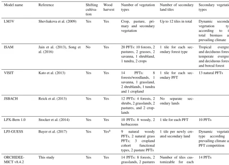
More and more DGVMs started to include gross transi-tions and we provide an overview of them in Table 1. All models in Table 1 include shifting cultivation and wood har-vest except that shifting cultivation is not included in ISAM, and five of them include sub-grid secondary land tiles when accounting for LUC. A recent review by Arneth et al. (2017)
found that including processes that have been previously ne-glected in DGVMs, including gross transitions and other land management processes such as crop harvest and manage-ment, can lead to an upward shift of estimated LUC emis-sions. Their study thus highlights the importance of includ-ing these processes. Furthermore, to more robustly account for shifting cultivation and wood harvest, which often have a certain rotation length and mainly involve secondary forests of different ages, it is critical for DGVMs to include sub-grid differently aged land cohorts. This feature exists in some DGVMs that combine with a forest gap model (e.g. LPJ-GUESS; Bayer et al., 2017) but it would be difficult to repre-sent forest species change because different tree plant func-tional types (PFTs) are mixed over a model grid cell. The same also applies for LM3V (Shevliakova et al., 2009). Other so-called area-based DGVMs (Smith et al., 2001) such as ISAM (Jain et al., 2013) and LPX-Bern 1.0 (Stocker et al., 2014) included secondary land tiles in the model but their capability to represent different rotation lengths in land use is limited. In the ORCHIDEE model, sub-grid forest cohorts have been recently included in the ORCHIDEE-CAN branch mainly for forest management purposes (Naudts et al., 2015), but a combination of both sub-grid land demography and gross land transition is still missing.
Here we present the new model developments in OR-CHIDEE that combine both sub-grid land cohorts and gross LUC. The objectives of this study are (1) to document a new LUC module, including sub-grid vegetation cohorts, forest harvest, and gross LUC in the ORCHIDEE model, that can be run with and without sub-grid age dynamics; (2) to doc-ument through an idealized pixel simulation the simulated carbon fluxes from shifting cultivation or land turnover be-tween model set-ups with and without sub-grid age dynam-ics; and (3) to document the model behaviour and forest age dynamics associated with the historical changes in LUC ac-tivities. Whereas the current paper focuses on documenting new model developments and subsequent changes in model behaviour, a companion paper presents a global reanalysis of historical LUC emissions (Yue et al., 2017).
2 Methods
2.1 Model developments to include sub-grid vegetation cohorts and gross transitions
2.1.1 Original land use change module with net transitions only
atmo-Table 1.An overview of DGVMs with implemented gross land use change (shifting cultivation) and forest wood harvest.
Model name Reference Shifting
cultiva-tion
Wood harvest
Number of vegetation types
Number of secondary land tiles
Secondary vegetation types
LM3V Shevliakova et al. (2009) Yes Yes Crop, pasture, pri-mary and secondary vegetation
Up to 12 tiles in total Dynamic secondary vegetation type according to the total biomass and prevailing climate ISAM Jain et al. (2013), Song et
al. (2016)
No Yes 20 PFTs: 10 forests, 2 pastures, 2 grasses, 2 savanna, 1 shrubland, 1 tundra, 2 crops
1 tile for each sec-ondary forest type
Tropical evergreen and deciduous forests, temperate evergreen and deciduous forests, and boreal forest
VISIT Kato et al. (2013) Yes Yes 14 PFTs: 8
forests/woodlands, 1 savanna, 1 grassland, 2 shrublands, 1 tundra and 1 cropland
1 tile for each sec-ondary PFT
13 natural PFTs
JSBACH Reick et al. (2013) Yes Yes 12 PFTs: 4 forests, 2
shrubs, 2 grasslands, 2 pastures, and 2 crop-lands
No separate sec-ondary lands
LPX-Bern 1.0 Stocker et al. (2014) Yes Yes 10 PFTs: 8 woody, 2 herbaceous
1 tile for each PFT 10 PFTs
LPJ-GUESS Bayer et al. (2017) Yes Yesa 9 natural woody
PFTs, 2 natural grass PFTs; 3 cropland cohort functional types, 2 pasture PFTs
1 tile per newly cre-ated secondary land
Dynamic vegetation type according to prevailing climate and PFT competition
ORCHIDEE-MICT v8.4.2
This study Yes Yes 14 PFTs: 8 forests, 2
grasslands, 2 pastures and 2 croplands
Number of tiles cus-tomizable for each PFT
14 PFTs
aWood harvest was not included in Bayer et al. (2017).
sphere. The carbon module simulates vegetation carbon cy-cle processes, including photosynthesis, photosynthate allo-cation, vegetation mortality and recruitment, phenology, lit-ter fall, and soil carbon decomposition. ORCHIDEE-MICT is a branch initially focusing on improving high-latitude pro-cesses (e.g. soil freezing, snow propro-cesses, permafrost dynam-ics, and northern wetlands) but is now under development to include more processes. Of interest for this study is that the grassland management module developed in Chang et al. (2013) is included (r2615). This allows for distinction be-tween natural grassland and pasture that have been mixed together in previous LUC simulations by ORCHIDEE.
In ORCHIDEE, land cover types are represented as PFTs, with each PFT being associated with a set of parame-ters. A typical model simulation consists of two stages: a spin-up stage with stable or constant forcing data until the model reaches an approximately equilibrium state, to mimic an era with no appreciable human perturbation, and a transient stage in which the model is forced with tempo-rally varying forcings (e.g. climate, atmospheric CO2, land
cover). The LUC module prior to this study accounts for net transitions only (Piao et al., 2009a) and has been used
in many applications (e.g. CMIP5, https://portal.enes.org/ models/earthsystem-models/ipsl/ipslesm; TRENDY, Sitch et al., 2015). To simulate historical LUC, a spin-up run is ini-tiated with a given initial land cover map (i.e. a PFT map), and then vegetation distribution is updated annually with pre-scribed PFT map time series during the transient simulation. The LUC module simply compares grid cell fractions of dif-ferent PFTs between the current simulation year and the next year. Then 12 vegetative PFTs (all standard model PFTs ex-cluding the bare soil PFT) are separated into two groups with expanding versus contracting areas. Carbon stocks and asso-ciated carbon fluxes on shrinking PFTs are displaced to ex-panding PFTs in proportion to their respective surface incre-ments.
2.1.2 Concept of gross transitions in relation to vegetation age structure
dif-Forest
Crop Young forest
Young crop
Forest Crop
Forest patch after merging (carbon stock
diluted) Forest
(intact) Crop
crop
Cropland after merging (carbon stock diluted) Net
Gross Merging due to single
patch representation
(a) (b)
(c) (d)
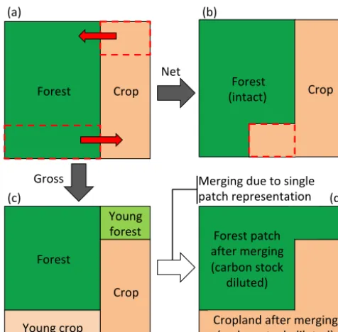
Figure 1.Schematic illustration of gross versus net land use change, with each land cover type being represented using a single patch within a model grid cell. The figure is adapted from Stocker et al. (2014).(a)Original fractions of forest and cropland before land use transitions. Dashed red rectangles indicate areas subject to LUC and red arrows indicate land flow direction. Here LUC consists of a net loss in forest and a simultaneous bidirectional flow between forest and cropland.(b)Post-LUC fractions of forest and cropland following the original LUC scheme of net transitions only in OR-CHIDEE. Bidirectional land flow is omitted, with only cropland area being expanded to account for its net increase as a result of the net forest loss, as indicated by the dashed red rectangle. The soil carbon stock of the new cropland patch is an area-weighted mean between that of the original cropland and the legacy stock from the former forest. Carbon stock of the remaining forest patch is left in-tact.(c)Intermediate post-LUC land cover pattern after account-ing for gross transition. Both the net loss of forest and bidirectional land flows are accounted for, with two young patches of forest and cropland being established.(d)Final state of post-LUC land cover after accounting for gross LUC with no sub-grid cohorts. The car-bon stocks of the remaining (original) forest and the newly created forest are immediately merged following LUC because there are no sub-grid cohorts. The same applies for cropland as well. Note that although forest and cropland fractions are ultimately the same as in
(b), the carbon densities are different.
ference between the two LUC schemes: one accounting for net transitions only (Fig. 1b), and the other accounting for gross transitions but with no sub-grid cohorts (Fig. 1c, d). Although the areas of forest and cropland after LUC are iden-tical (Fig. 1b, d), carbon stocks for the same vegetation type (e.g. forest) are different between the two schemes. Accord-ing to the net transition scheme, the carbon stock of the fi-nal forest patch shown in Fig. 1b remains intact. But under the gross scheme (Fig. 1d), the post-LUC forest carbon stock
Primary
Crop Secondary
Primary crop
Secondary
Very young forest
Young crop with high soil C
Primary
Crop Secondary
Primary
Crop Secondary
Young crop with low soil C
Very young forest
(a) (b)
(c) (d)
Figure 2.Gross land use change involving forests with different ages under a model scheme capable of representing sub-grid land cohorts. The figure is adapted from Stocker et al. (2014). LUC here is similar to in Fig. 1, except that forest is no longer a single ageless patch but consists of two patches of primary and secondary forests, i.e. having an age structure.(a)The same area of forest is converted to cropland as in Fig. 1a but conversion is made from primary forest.
(b)Consequently, a young cropland patch with rich legacy forest soil C is established. Meanwhile, a very young forest patch is estab-lished due to the bidirectional gross land flux. Because the model uses multiple sub-grid patches to represent vegetation age structure (or differently aged cohorts), merging of patches with different car-bon stocks is no longer necessary. Panel(c)shows an alternative to(a)in which conversion of forest to cropland is made on a sec-ondary forest. Correspondingly, in(d), which shows the post-LUC state of(c), the established young cropland patch will have lower legacy soil C than that in(b).
is an area-weighted mean between the original forest patch not being impacted by LUC and the newly established forest with a low carbon density that results from cropland aban-donment. Consequently the carbon stock of the grid cell is expected to be smaller in Fig. 1d than in 1b and LUC carbon emission in Fig. 1d is conversely larger than in Fig. 1b.
Figure 1c represents the real land cover state after LUC, while the merging shown in Fig. 1d is only a necessary sim-plification when no sub-grid cohorts are represented in the model. Ideally, the model capability could be expanded to in-clude cohorts to represent the real world case as in Fig. 1c. In addition, inclusion of sub-grid cohorts would allow not only the distinction between original intact forest and newly estab-lished forest but also among different forest cohorts (e.g. pri-mary versus secondary forests) regarding which forest patch to be cleared for cropland.
mul-tiple patches within a grid cell are used to represent cohorts of a single vegetation type but with different ages since es-tablishment. These cohorts often have different carbon stocks either due to different lengths in carbon accumulation time (e.g. for forest) or due to different extents to which legacy soil carbon is present (e.g. for croplands establishing on for-mer forests). The areas subject to gross LUC transition in Fig. 2a and b remain the same as in Fig. 1a (dashed red rectangles), but primary and secondary forests are cleared in Fig. 2a and b, respectively. Thus, LUC emissions from clearing of primary forest are expected to be higher due to its higher biomass stock. Correspondingly, the legacy soil car-bon stocks on the cohort of new cropland are also higher (shown in Fig. 2b and d).
Figures 1 and 2 have shown the example of LUC transi-tions between forest and cropland, but other types of LUCs, including forest harvest, can be handled in a similar way. In the case of forest harvest, having cohorts avoids the simpli-fication of merging a young re-established forest after har-vest with the original forest, which serves as the exact source of harvest. This can effectively simulate forest management practices that induce rotations of different forest cohorts (e.g. see McGrath et al., 2015, for a forest management history in Europe).
2.1.3 Expansion of ORCHIDEE-MICT capacity to represent sub-grid vegetation cohorts
In order to simulate gross LUC combined with sub-grid vegetation cohorts as illustrated in Fig. 2, we expanded the ORCHIDEE-MICT capability to include sub-grid evenly aged cohorts. This necessitates multiple patches within a grid cell for a single PFT, which inherits most of the parameters from its parent PFT (they still belong to the same PFT and thus are largely physically similar). These patches are named cohort functional types (CFTs) here, to be distinguished from the original plant functional types. In this sense, the origi-nal PFTs actually become “meta-PFTs” which were named meta-classes (MTCs). As subsequent LUCs generate differ-ently aged CFTs, the computational demand will be greatly increased. Hence, the number of CFTs within an MTC is lim-ited to a user-defined number.
ORCHIDEE-trunk has a feature called “PFT externaliza-tion” that allows the creation of a new user-specified PFT by inheriting its parameters from an existing one. A user can then modify specific parameters at their convenience. Based on this feature, the ORCHIDEE-CAN branch (the svn revi-sion number is 2566; Naudts et al., 2015, p. 2037) has devel-oped representation of sub-grid forest age classes (i.e. equiv-alent to our CFTs here). Each forest age class is an inheri-tance of a given forest MTC. There, the transitions from one age class to another were defined by tree diameters. When a forest of a certain age class reaches its diameter limit, it moves into the next age class, and is merged with the exist-ing forest patch of that age class if there is one. All
associ-ated biophysical and biogeochemical variables are merged as well following an area-weighted mean approach with a few exceptions for discrete variables such as the applied forest management strategy.
ORCHIDEE-MICT also inherits this externalization fea-ture from ORCHIDEE-trunk. Here we ported the codes of forest age class functionality from ORCHIDEE-CAN to develop the CFT functionality needed for LUC simu-lation with cohorts in ORCHIDEE-MICT. The code base to include sub-grid forest cohorts was migrated from ORCHIDEE-CAN, with substantial adaptions being made in ORCHIDEE-MICT. Except for this, all other LUC develop-ments have been achieved within the current study. Contrary to ORCHIDEE-CAN (see above), ORCHIDEE-MICT uses woody biomass to delimit different forest cohorts, with older cohorts having a higher woody biomass. Forest grows old by moving from the current cohort to the next one when the woody biomass exceeds the cohort upper boundary. Except for the cohort boundaries, no further cohort-specific param-eterizations have been performed, so essentially all cohorts are governed by the same set of biophysical and ecological parameter values. However, in ORCHIDEE-MICT there are indeed some simple aging processes to proximate the key changes when a forest grows old: notably, the net primary production (NPP) allocation to below-ground sapwood de-creases with the time since establishment.
In addition, we expanded the concept of CFT to crop-lands, natural grasscrop-lands, and pastures. Cohorts are defined with their soil carbon stocks for these herbaceous vegetation types; this is a definition relevant to LUC emission calcu-lation. Because the directional change of soil carbon largely depends on the vegetation types before and after LUC and on climate conditions (Don et al., 2011; Poeplau et al., 2011), ideally agricultural cohorts from different origins should be differentiated. However, to avoid inflating the total number of cohorts and the associated computational demand, as a first attempt, we simply divide each herbaceous MTC into two broad sub-grid cohorts according to their soil carbon stocks and without considering their individual origins. We expect that such a parameterization can accommodate some typical LUC processes, such as the conversion of forest to cropland where soil carbon usually decreases with time, but not all LUC types (for instance, soil carbon stock increases when a forest is converted to a pasture). The biomass or soil carbon thresholds that delineate different CFTs must be properly pa-rameterized in order to have sensible CFT segregation within different contexts of land use change. This will be further de-tailed in Sect. 2.2.3. In practice, for single-site simulations, the parameterization could be set up via a configuration file enumerating the thresholds for all CFTs. For regional appli-cations, an input file containing spatially explicit thresholds will be used.
Tier 1 Tier 2: meta-class Tier 3: CFT Tier 3: CFTTier 2: cohort Tier 1
MTC1 (bare soil) CFT1,1
CFT2,1 CFT2,1
CFT2,2 …
… CFT9,1
CFT2,6 CFT3,1
CFT3,2 CFT2,2
… …
CFT3,6 CFT9,2
… … …
CFT9,1
CFT9,2 CFT2,6
… …
CFT9,6 CFT9,6
CFT10,1 CFT10,1 CFT10,2 CFT11,1 CFT11,1 CFT10,2 CFT11,2 CFT11,2 CFT12,1 CFT12,1 CFT12,2 CFT13,1 CFT13,1 CFT12,2 CFT13,2 CFT13,2 CFT14,1 CFT14,1 CFT14,2 CFT15,1 CFT15,1 CFT14,2 CFT15,2 CFT15,2
GrasslandMTC10 (C3 grassland) Grassland
MTC11 (C4 grassland)
Forest
MTC2 (tropical broadleaf evergreen)
Forest MTC3 (tropical
broadleaf raingreen)
MTC9 (boral needleaf deciduous)
Pasture MTC12 (C3 pasture) Pasture
MTC13 (C4 pasture)
Cropland MTC14 (C3 cropland) Cropland
MTC15 (C3 cropland)
Cohort f,1
Cohort f,2
Cohort f,6
Cohort g,1
Cohort g,2
Cohort p,1
Cohort p,2
Cohort c,1
Cohort c,2
Model parameterizaIon hierarchy LUC hierarchy
(a) (b)
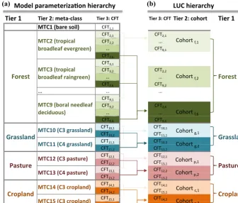
Figure 3.Two parallel hierarchies from the model parameterization and land use change perspective.(a)Sub-grid cohort function types (CFTs) as inheritances of meta-classes (MTCs) and the corresponding parameterization hierarchy. There are in total 14 vegetative MTCs corresponding to four vegetation types. The notation of CFTi,j indicates that it inherits from MTCiand belongs to thejth cohort (Cohortj). Each forest MTC has six cohorts, with Cohort1being the youngest and Cohort6the oldest, whereas each herbaceous MTC is set tentatively to have two cohorts. Darker colours indicate older cohorts.(b)Within the gross LUC module hierarchy, Tier 3 remains the level of CFT, but CFTs are reorganized to derive the Tier 2 information based on the level of cohorts under the same Tier 1 as in(a). A cohort baring the notation of Cohortv,i indicates it belongs to vegetation type “v” (where “v” could be forest, natural grassland, pasture, or cropland) and meta-class “i”. This reorganization of the hierarchy from the left to the right side is to prepare for properly allocating prescribed LUC transitions first onto the cohort level, then further to different CFTs within each cohort.
hierarchy corresponds to the four basic vegetation types (for-est, natural grassland, pasture, and croplands, abbreviated as f, g, p, and c respectively). Tier 2 corresponds to meta-classes in ORCHIDEE-MICT, which contain one bare soil MTC and 14 vegetative MTCs, with each vegetative MTC belonging to one of the four basic vegetation types. Tier 3 corresponds to CFTs. A CFT is noted as CFTi,j to denote that it
inher-its inher-its parameter values from the MTCi and belongs to the
jth cohort. For this study, forest MTCs contain six CFTs and herbaceous MTCs contain two CFTs. The number of CFTs for each MTC is not hard-coded in the model and can be specified by users via a configuration file.
With sub-grid cohorts, the model spin-up run is initiated with an input MTC map, essentially the same as in the case without sub-grid cohorts (recall that in Sect. 2.1.1 this MTC map is called a PFT map). But the difference is that the ini-tial prescribed areas (as fractions of grid cell area) of differ-ent MTCs are all assigned to their youngest cohorts. During model spin-up forest woody mass will grow to exceed the
thresholds of the first cohort, so that forests will move to the second cohort, and so on. At the end of spin-up, all forests thus end up in the oldest cohort of each MTC. The same case applies to herbaceous MTCs, given that cohort thresholds are properly defined (see more details in Sect. 2.2.3).
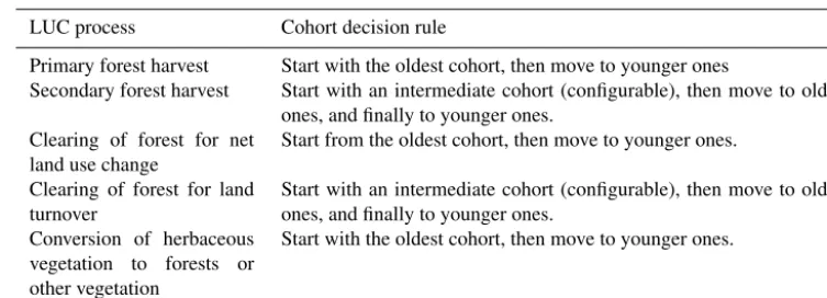
Table 2.A set of implemented rules regarding cohort selection for different land use change processes.
LUC process Cohort decision rule
Primary forest harvest Start with the oldest cohort, then move to younger ones
Secondary forest harvest Start with an intermediate cohort (configurable), then move to older ones, and finally to younger ones.
Clearing of forest for net land use change
Start from the oldest cohort, then move to younger ones.
Clearing of forest for land turnover
Start with an intermediate cohort (configurable), then move to older ones, and finally to younger ones.
Conversion of herbaceous vegetation to forests or other vegetation
Start with the oldest cohort, then move to younger ones.
recruitment does not modify forest cohort ground coverage. In addition, forest mortality and subsequent regeneration due to forest fires are handled in a similar manner. ORCHIDEE-MICT has integrated a prognostic fire module to simulate open grassland and forest fires arising from both natural and anthropogenic ignitions (Yue et al., 2014). Other forest disturbances, such as wind-throw, diseases, and insect out-breaks, are not explicitly considered in ORCHIDEE-MICT. Because of these reasons, after the spin-up, the only way to create secondary cohorts in the model is through LUC.
When entering transient simulations with LUC, younger cohorts will begin to be created. From a modelling perspec-tive, the oldest cohorts in ORCHIDEE-MICT are somewhat equivalent to the primary lands (especially, the oldest forest cohorts are equivalent to primary forests), and other younger cohorts are analogue to secondary lands.
2.1.4 Model developments to include gross land use change and forest harvest, with and without sub-grid cohorts
This section describes the implementation of gross LUC and forest harvest with sub-grid CFTs. We focus on the imple-mentation with sub-grid cohorts because the same LUC pro-cess without cohorts could be simply treated as a particular case in which all MTCs have only one single cohort. The module interface is designed to receive forcing information on land area fluxes among four basic land cover types of for-est (f), natural grassland (g), pasture (p), and cropland (c), taking into account the current LUC modelling landscape in DGVMs (as briefly reviewed in the introduction) and the availability of LUC reconstructions (e.g. Hurtt et al., 2011). The present developments are intended for the case in which changes in vegetation coverage are only driven by histori-cal LUC activities and so there is no need to use the dy-namic vegetation module of ORCHIDEE. This is different from the LUC implementation in JSBACH DGVM in Reick et al. (2013) in which a lot of effort has been devoted to rec-onciling the vegetation types in the forcing data (primary and secondary natural lands in the Land-Use Harmonization data
set version 1 or LUH1 data) and the vegetation distributions simulated by the dynamic vegetation module of JSBACH. We focus on including sub-grid land cohorts in the model and implementing a set of hierarchical rules for which land cohorts are subjected to different LUC processes (Table 2). The allocation of natural lands into forest versus grasslands in the model, and the reconciliation of LUH1 land cover dis-tribution and model PFT map, are instead handled by inde-pendent preparations of reconstructed historical land cover map time series.
In order to compare the simulation results from the gross LUC module with the original net-transition-only LUC mod-ule, we separate the gross LUC areas into two additive terms: net change equivalent to the original net transition (pre-scribed by the matrixMnet) and land turnover for the
bidirec-tional equal land fluxes between any pair of land cover types (prescribed by the matrixMturnover). Similarly, the forest
har-vest information is prescribed in a third matrixMharvest. For
the moment, information for all three LUC types is provided as a fraction of grid cell area. This is a deliberate choice, mainly for the convenience of progressive stage-wise model development. We will come back to the influence of this choice within the land use decision contexts in Sect. 4.
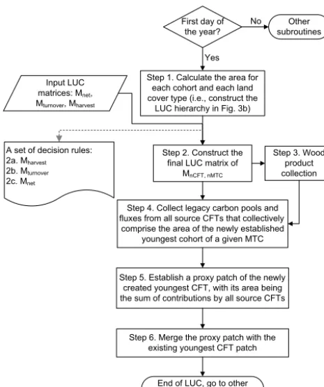
The key processes of the gross LUC module with CFTs are shown in Fig. 4, comprising in total six steps. The LUC mod-ule is called at the first day of each year. Input data are the three matrices.MnetandMturnover are both square matrices
with a size of 4 by 4:
,
First day of
the year? subroutinesOther No
Yes
Step 1. Calculate the area for each cohort and each land cover type (i.e., construct the
LUC hierarchy in Fig. 3b)
Step 2. Construct the final LUC matrix of
MnCFT, nMTC Input LUC
matrices: Mnet, Mturnover, Mharvest
Step 4. Collect legacy carbon pools and fluxes from all source CFTs that collectively
comprise the area of the newly established youngest cohort of a given MTC
Step 3. Wood product collection
Step 5. Establish a proxy patch of the newly created youngest CFT, with its area being the sum of contributions by all source CFTs
Step 6. Merge the proxy patch with the existing youngest CFT patch
End of LUC, go to other subroutines A set of decision rules:
2a. Mharvest 2b. Mturnover 2c. Mnet
Figure 4. Schematic representation of the new LUC scheme in ORCHIDEE-MICT v8.4.2 accounting for net land use change, land turnover, and forest harvest in combination with sub-grid cohort representation.
where the elementFi>jdenotes the land flux from land cover
typeitoj, withiandj being elements of the vector of [f g p c]T. The diagonal elements correspond to land fractions intact from any land use transitions and are simply ignored in the LUC module. By definition,Mturnover is a symmetric
square matrix.Mharvestis a matrix with only two elements:
harvest area from primary and secondary forests.
As explained in Sect. 2.1.3, the construction of CFTs within the model follows the model parameterization hier-archy shown in Fig. 3a. The cohort age subjected to LUC is one of the most important considerations in LUC decisions, especially in the context of land turnover and forest harvest. This necessitates a re-organization of the CFTs to derive the LUC hierarchy shown in Fig. 3b, in which Tier 2 informa-tion is about areas of different cohorts of the same land cover type, and Tier 3 remains on the level of CFTs. Thus, Step 1 in the LUC module (Fig. 4) is to construct the LUC hierarchy, i.e. to calculate within the model the areas of each cohort for each vegetation type.
When implementing LUC matrices, all information of land transitions between the four basic land cover types must first be downscaled on the cohort tier (i.e. decision on which cohort is subjected to LUC) and then on the CFT tier (i.e. how LUC-affected area is distributed among
differ-ent comprising meta-classes within each cohort; refer also to Fig. 3b). This is achieved in Step 2 as shown in Fig. 4. Be-cause all the newly established lands, regardless of their orig-inating LUC process, must belong to the youngest CFT of the MTCs that comprise the target land cover type, the ultimate outcome of Step 2 is a single (large) matrix MnCFT,nMTC
(nCFT: no. of CFTs; nMTC: no. of MTCs), which indicates the area transferred from each CFT to the youngest cohort of the MTC concerned. The rules to convert LUC matrices into components ofMnCFT,nMTC depend on LUC types and will
be explained in detail later. But as long as Step 2 is finished, the remaining steps are rather straightforward.
Step 3 handles forest wood collection (here “collection” rather than “harvest” is used, to avoid the confusion with for-est wood harvfor-est, which is a means of forfor-est management), from forest being converted to other land cover types, and forestry harvest (forest remaining forest). We assume that a certain fraction of above-ground woody biomass (i.e. sap-wood and heartsap-wood) is lost as instant CO2flux into the
at-mosphere (i.e. due to on-site disturbance), and that the re-maining wood is collected as wood product pools. Step 4 in-volves the proper displacement of associated carbon stocks and fluxes from the donating CFTs to the newly established (youngest) cohorts of MTCs, after wood collection. Notably, the legacy carbon stocks in litter and soil collected from the donating CFTs are transferred to the newly established youngest CFTs. Then in Step 5, each youngest CFT cohort is established and initialized, with its fraction of grid-cell area being the sum of contributing areas given by each source CFT. Finally, in Step 6, a newly established cohort is merged with the existing youngest CFT cohort if there is one. When merging stocks or fluxes between the newly established and existing CFTs, an area-weighted mean approach is followed: xmerged=
xnew×areanew+xexisting×areaexisting
areanew+areaexisting
, (2)
wherex is the variable in question (e.g. leaf biomass, soil carbon stock),xnew andxexistingare the values of the newly
established patch and the existing patch before merging re-spectively, andxmergedis the value of the composite patch
af-ter merging. The variables areanewand areaexistingare patch
areas of the newly established patch and the existing patch respectively.
We now return to Step 2, explaining the different rules used to build theMnCFT,nMTCcomponents for different LUC
types. We start withMharvest by assuming that it precedes
for-est area and harvfor-ested biomass in LUH1. Here we used the area information (a deliberate choice that will be discussed in Sect. 4). Because of this, ensuring the consistency between the harvest area in the forcing and that being actually real-ized in the model is an important consideration. Moreover, as we want to compare simulated LUC impacts between the two model configurations with and without sub-grid cohorts, it is necessary to ensure that exactly the same LUC area is re-alized in both configurations. This involves a set of decision rules to properly allocate the prescribed harvest area into dif-ferent forest cohorts (Table 2).
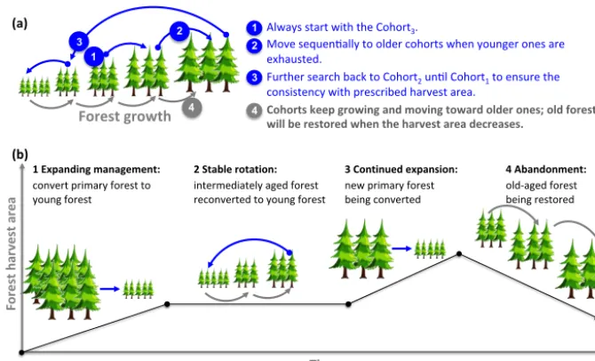
Implementation of primary forest harvest is straightfor-ward: we always start with the oldest cohort and move se-quentially downwards to younger ones if older cohorts are exhausted until the prescribed harvest demand is fulfilled (Table 2). For secondary forest harvest, we start with inter-mediately aged cohorts. But if the existing area of interme-diately aged cohorts is not sufficient to fulfill the prescribed harvest area, we are left with two options to either search up-wards for older cohorts or downup-wards for younger ones. We decide to first search upward and then search downward, if all cohorts older than the intermediate age still cannot ful-fill the prescribed harvest demand (Table 2). This rule allows potential temporal changes in harvested area to be accommo-dated, as explained in Fig. 5. Under such a scheme, (1) at the very beginning (after spin-up) and before the existence of any secondary forests, harvest will start with the oldest cohort, i.e. corresponding to harvest of primary forests (sometimes, because of the inconsistency between the input harvest infor-mation and existing forest cohort structure in the model, sec-ondary forest harvest could be prescribed for pixels in which only primary forests exist in the model). (2) If harvest area of secondary forests remains stable, then as soon as sufficient intermediately aged cohorts are created via conversion of pri-mary forest to regrowing younger cohorts, a corresponding stable rotation cycle would be maintained in the model as well. (3) If the harvest area increases, the upward searching would allow additional harvest of primary forests (i.e. area subject to the stable rotation is expanded). (4) If the harvest area decreases, moving cohorts from younger to older ones independent of any LUC activities would allow the restora-tion of older cohorts – e.g. a consequence of abandonment of forest management. (5) Finally, the downward searching for younger cohorts after exhausting all other older cohorts is solely to ensure the consistency between prescribed input harvest area and that actually realized in the model. Hence, this scheme is designed in order to faithfully implement the prescribed harvest areas in the model with an explicit con-sideration of forest successional states (i.e. primary or sec-ondary). But when this is not possible because of inevitable mismatch between the model and forcing data, harvest areas of primary and secondary forests could mutually compensate for each other in the model to ensure that their prescribed to-tal harvest area remains realized.
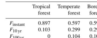
Table 3.Fractions of above-ground woody biomass lost immedi-ately to the atmosphere during a forest clearing and channelled to 10- and 100-year turnover wood product pools. These fractions are different depending on forest biomes.
Tropical Temperate Boreal
forest forest forest
Finstant 0.897 0.597 0.597
F10 yr 0.103 0.299 0.299
F100 yr 0 0.104 0.104
A number of studies reported that fallow lengths for shift-ing cultivation could range from a few years to more than 50 years depending on different regions, with the majority being 10–40 years (Bruun et al., 2006; Mertz et al., 2008; Thrupp et al., 1997; van Vliet et al., 2012), and there is a tendency in reduction of fallow lengths possibly because of increased population pressure (van Vliet et al., 2012). Hurtt et al. (2011) assumed a mean residence time of 15 years for shifting cultivation for tropical regions in the LUH1 re-construction data. Based on these reports, we assume forest clearance for shifting cultivation to occur primarily in sec-ondary forests and treat it similarly as secsec-ondary forest har-vest when allocating the prescribed LUC area into different cohorts (Table 2). The only difference is that the destination land cover remains forest in the case of forest harvest but is agricultural land in the case of shifting cultivation. For all other land transfers in shifting cultivation (e.g. pasture to for-est), we start exclusively from the oldest cohort and move downwards to younger ones (Table 2). For net LUC, prior-ity is again given to older cohorts followed by younger ones (Table 2).
Finally, we still need to downscale the LUC area in each cohort to its component CFTs. This is done by allocating the LUC area in each cohort to its member CFTs in proportion to the existing area of each CFT.
2.1.5 LUC processes that remain unchanged in the model
ORCHIDEE simulates two wood product pools with a turnover length of 10 years and 100 years. Fractions of above-ground woody biomass as instant on-site losses (Finstant) and entering into the two wood product pools
(F10 yr, F100 yr) follow the values in the original
Fo
re
st
h
ar
ve
st
a
re
a
1 Expanding m anagement:
convert primary forest to young forest
2 Stable rotation: intermediately aged forest reconverted to young forest
3 Continued e xpansion:
new primary forest being converted
4 Abandonment:
old-aged forest being restored
Time
Always start with the Cohort3.
Move sequen@ally to older cohorts when younger ones are exhausted.
Further search back to Cohort2 un@l Cohort1 to ensure the consistency with prescribed harvest area.
Cohorts keep growing and moving toward older ones; old forests will be restored when the harvest area decreases.
Forest growth
1 2
3
4
(a)
(b)
4 1
2 3
Figure 5.Rules of selection of forest cohorts in secondary wood harvest to account for the dynamics in harvest area over time.(a)Rules of selection of forest cohorts (blue arrows). Clear-cut harvest (1) first starts with intermediately aged cohort, then moves to older cohorts until the oldest one; (2) if the prescribed harvested area still cannot be satisfied, then the harvest will move back to the even younger cohorts (3) to the youngest one until the prescribed harvested area is fulfilled. Independent of the harvest activity is the movement of forests from younger cohorts to older ones because of growth (grey arrows).(b)Example of cohort dynamics along with temporal changes in the harvest area shown in the black curve: (1) before the onset of any harvest activity (i.e. after the model spin-up), only the oldest cohorts are available so harvest starts with the primary forest; (2) for a stable harvest area, a steady-state cycle involving only secondary forest is established (intermediate secondary cohorts being harvested is represented by the blue arrow, and younger growing cohorts are represented by grey arrows); (3) then with an increase in harvest area, more primary forests are harvested; (4) finally, in this example, the harvest area decreases, and older cohorts are restored.
Other processes relevant to LUC are left unchanged with the original model version. In particular, crop harvest is ap-plied to cropland CFTs with a fraction of 45 % of biomass turnover being harvested in the model and exported outside the ecosystem (Piao et al., 2009a). Pasture CFTs are also har-vested in the same fashion. Agricultural harvest and associ-ated fluxes to the atmosphere through food consumption or livestock feeding are assumed to happen locally in the model during the same year of harvest, without considering spa-tial relocation through international trade. Fires are simulated with a prognostic module, but as explained in Sect. 2.1.3, fire disturbances do not lead to creation of young cohorts, but only their carbon consequences (e.g. emissions, vegetation mortality) are included.
2.2 Simulation set-up
2.2.1 Definition of land-use change emissions (ELUC)
and carbon flux sign convention
The land carbon balance simulated by ORCHIDEE-MICT v8.4.2 (i.e. net biome production or NBP), when land use change is included, is defined as
NBP=NPP+FInst+FWood+FHR+FFire+FAH+FPasture,
(3)
where NPP is the net primary production, and all fluxes with Fdenoting outward carbon fluxes from the land system (they are assigned a negative sign following the ecosystem conven-tion, indicating that carbon is lost from ecosystems), with FInstfor the instantaneous carbon flux during LUC (e.g.
car-bon release arising from site preparation, land-clearing burn-ing),FWoodfor the delayed carbon release due to wood
prod-uct degradation,FHRfor heterotrophic respiration from litter
and soil organic carbon decomposition,FAH for agricultural
harvest on both croplands and pastures, andFPasturefor
car-bon sources from pastures other than harvest, i.e. export of animal production and methane emissions (see Chang et al., 2015, for details).FInstandFWoodare both fluxes on an
an-nual timescale that depend only on wood mass at the time of forest clearing and the respective wood product degrada-tion rates (see Sect. 2.1.5).FHRis simulated at a time step of
30 min and depends on soil temperature and moisture.FFire
is simulated with a prognostic fire module SPITFIRE (Yue et al., 2015).
The LUC emissions (ELUC) are quantified as the
differ-ence in simulated NBP between two paired simulations, with LUC (or a specific LUC process) included in one simulation but not the other one:
where NBPLUCand NPBcontrol are NBP simulated with and
without LUC. A negative ELUCdenotes a carbon source to
the atmosphere, i.e. the ecosystem carbon sink is reduced be-cause of LUC. This definition follows Pongratz et al. (2014, p. 178) and is also the same as used in TRENDY (Sitch et al., 2015) simulations and the existing global carbon budget analysis (Le Quéré et al., 2016). As explained by Pongratz et al. (2014), such a definition quantifies the net LUC flux because it integrates both emissions to the atmosphere (e.g. deforestation) and uptakes by potentially recovering vegeta-tion (e.g. agricultural abandonment). More specifically, this corresponds to the definition “D3” using uncoupled DGVM simulations in Pongratz et al. (2014, Eq. 15c, p. 187), which contains instantaneous fluxes, legacy fluxes, and “loss of ad-ditional sink (source) capacity (LOAS)”.
Instantaneous fluxes refer to the carbon emissions directly arising from LUC, often occurring within the first year since LUC (FInstin our case). Legacy fluxes arise from the
read-justment of carbon stocks to the new type of vegetation and/or the changes in management intensity over time (Pon-gratz et al., 2014), and LOAS refers to the carbon sink– source difference between the actual land cover after LUC and the otherwise potential one under environmental pertur-bations. All other flux terms on the right side of Eq. (3) ex-cept FInst contribute to the legacy fluxes and LOAS. Here,
as our model development mainly distinguishes the biomass carbon of secondary forests, it is expected that FInst and
FWood will be the major fluxes to influence the simulated
ELUC. To facilitate the demonstration of model behaviour,
we refer to FInst andFWood collectively as LUC-associated
direct fluxes and their variations will be examined in detail by using an idealized grid cell simulation.
The model developments presented here enable us to make two parallel simulations that include LUC: with and without sub-grid age dynamics. Their simulated ELUC can thus be
compared to separate the effect of including sub-grid age dy-namics. Henceforth, for briefness, we denote the simulation without sub-grid age dynamics as Sageless and the one with
age dynamics asSage.
2.2.2 Idealized simulation on a single grid cell
We conducted an idealized grid cell simulation with pre-scribed land cover and LUC matrices to compare in de-tail the simulated carbon pools and fluxes betweenSageand
Sageless. The geographical coordinates of the simulation site
are 9.25◦S, 18.25◦E on a 0.5◦global grid, in the north of An-gola, Africa, where the miombo woodlands are known to be subject to practices of shifting cultivation. The ESA CCI land cover map for the 5-year period of 2003–2007 (https://www. esa-landcover-cci.org/) shows a dominant fraction of tropi-cal deciduous broadleaf forest for this grid cell. Hence, for the idealized experiment, the initial vegetation composition is prescribed as 85 % tropical deciduous broadleaf forests and 15 % C4 croplands. As we will focus on the LUC impacts,
other model forcings (climate, atmospheric CO2, etc.) are
held constant, with climate input data recycling the year of 1901 (CRUNCEP v5.3.2 climate data) and atmospheric CO2
concentration being fixed at 350 ppm. The model is tested for a hypothetical scenario of constant annual land turnover with 5 % of grid cell area between forest and C4cropland. Forest
harvest of the same annual areal fraction is expected to have a largely similar impact. The spin-up was run for 450 years until biomass and soil C stocks reached equilibrium and the mean annual NBP was close to zero without including any LUC. Starting from the spin-up, a transient simulation with the prescribed LUC matrix was performed for 100 years. 2.2.3 Simulation over southern Africa
Subsequently, the model behaviour has been documented for a real-world case over the region of southern Africa (south from the Equator of the African continent). All three LUC types occurred historically in this region, making it ideal to demonstrate model behaviour regarding forest cohort dy-namics as presented in Fig. 5. This regional simulation serves a single purpose – to further exemplify model features that cannot be sufficiently demonstrated over a grid cell.
The regional simulation is performed at 2◦resolution for 1501–2005. We used the land use reconstruction from LUH1 covering 1501–2013 (Hurtt et al., 2011, http://luh.umd.edu/ data.shtml#LUH1_Data) re-gridded from the original 0.5◦to a 2◦spatial resolution. From the LUH1 data set we derived the matrices of the three types of LUC: net land use change, land turnover, and wood harvest. Land turnover information is extracted from LUH1 as the minimum land fluxes between two vegetation types. Wood harvest from primary and sec-ondary forests in LUH1 is used, while wood harvest from non-forest is not. Climate forcing data are from CRUNCEP-v5.3.2 at a 2◦resolution. For the spin-up, climate data were cycled from 1901 to 1910, with atmospheric CO2
concentra-tion fixed at the 1750 level (277 ppm). In the transient sim-ulation, atmospheric CO2concentration began to increase in
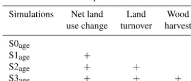
1750 and climate data were varied starting in 1901. The dy-namic vegetation module was turned off in order to apply the prescribed historical LUC. Factorial simulations are con-ducted to highlight changes in areas of different forest co-horts when different LUC processes are included, as shown in Table 4.
Each forest MTC has six CFTs to represent six cohorts. The woody mass thresholds are set in a way that they cor-respond roughly to the woody masses at ages of 3, 9, 15, 30, 50 years, and the mature or primary forest (with an age greater than 50 years) during the spin-up simulation for Cohort1to Cohort6respectively. The Cohort3with an age of
den-Table 4. Factorial simulations to examine forest cohort dynamics when including different LUC processes: net land use change, land turnover, and wood harvest. The plus signs (+) indicate that the corresponding processes (matrices) are included in the simulations. Only simulations with sub-grid age dynamics are carried out, with S0agehaving no LUC activities to S3age including all LUC pro-cesses.
Simulations and LUC processes included
Simulations Net land Land Wood
use change turnover harvest
S0age
S1age +
S2age + +
S3age + + +
sity. The CFT thresholds of soil carbon stock are the same for all herbaceous MTCs. We first calculate the maximum soil carbon stock of all MTCs (including the forest ones) at the end of spin-up for each grid cell, and cohort thresholds are then taken as this maximum value and its 65 % value. Be-cause the energy balance in ORCHIDEE-MICT is resolved for the average of all CFTs over a grid cell, and the hydrolog-ical balance is resolved for three sub-grid water columns (i.e. the water column of bare soil, forest, and herbaceous vegeta-tion), we expect the factors influencing soil carbon decompo-sition (e.g. soil temperature, soil moisture) to have little vari-ation among CFTs of the same MTC. This justifies the small number of herbaceous CFTs for the sake of computation effi-ciency. Overall, this feature of separating herbaceous MTCs into multiple cohorts is coded more as a placeholder for the current stage of model development rather than having solid scientific significance. Fully tracking soil carbon stocks of different vegetation types and their transient changes follow-ing LUC would require a much larger number of cohorts than used in this study.
3 Results
3.1 Grid cell simulations with and without sub-grid forest age dynamics
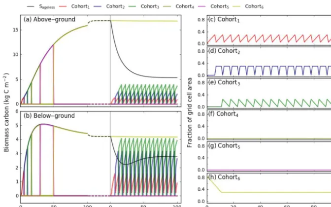
3.1.1 Temporal patterns of biomass carbon stock during the spin-up and transient simulations Figure 6a and b exhibit the evolution of above- and below-ground biomass for bothSagelessandSagesimulations for the
spin-up and transient simulation for a test grid cell located in Angola. The results for theSagesimulation are shown for
in-dividual cohorts (Cohort1to Cohort6). For this test an annual
forest–cropland turnover of 5 % of the grid cell area was im-posed. Figure 6c–h present changes in the ground fractional cover of different forest cohorts during the transient
simula-tion.SagelessandSageshare the same biomass accretion with
time during the spin-up, butSageshows a succession of forest
cohorts – with biomass moving from one cohort to the next (Fig. 6a, b). At the end of the spin-up, all biomass is found in Cohort6(i.e. the oldest cohort), with an initial forest cover of
85 %.
More differences emerge when entering the transient sim-ulation. Above-ground biomass in Sageless shows an initial
sharp drop followed by a more gradual decline under con-stant land turnover because biomass of the single forest patch is constantly diluted by merging with the new forest patch with a low biomass, which is established as a result of land turnover (see also Fig. 1). Below-ground biomass, how-ever, shows a corresponding initial drop but then slightly in-creases. Eventually, both above- and below-ground biomass stocks in Sageless reach a new equilibrium, which is lower
than their values at the end of the spin-up. By contrast, in Sage, the fraction of Cohort6 declines with the start of the
transient simulation because of conversion to cropland. This decline continues until the 12th year, after which the re-maining Cohort6covers only 30 % of the grid cell (Fig. 6h).
Younger cohorts are progressively created as forests restore after shifting agriculture abandonment, with the Cohort1(i.e.
the youngest one) appearing during the initial 6 years af-ter the start of LUC, afaf-ter which its biomass is moved into Cohort2(Fig. 6c, d). Cohort3starts to appear at the 12th year
when biomass in Cohort2moves into it. Then its coverage
de-clines as this cohort, rather than Cohort6, is used as the source
for shifting cropland, according to the model rule that sec-ondary forest is taken prior to primary forest in land turnover (Fig. 5). After the initial 15 years (the rough age of Cohort3),
the fractions of Cohort1, Cohort2, and Cohort3 reach a
dy-namic stable state. As Cohort3is being constantly converted
to cropland, it has never developed into Cohort4or Cohort5.
This explains the zero fractions of these two latter cohorts in Fig. 6f and g.
While the above-ground biomass continuously grows dur-ing the spin-up, the below-ground biomass first increases with time and then slightly declines before reaching the equilibrium value. This is because ORCHIDEE-MICT has a preferential allocation of NPP to below-ground sapwood when forests are young. The small decline in below-ground biomass in the late spin-up stage thus results from an almost stabilized NPP (under a big-leaf approximation), a reduced below-ground allocation, and a constant mortality. Because of this feature, ORCHIDEE-MICT creates a higher below-ground biomass in younger forest cohorts (e.g. Cohort2and
Cohort3in Fig. 6a and b) inSagethan the single forest patch
inSageless in the transient simulation. However, the
above-ground biomass in younger Cohort2and Cohort3 inSageis
lower thanSageless. The difference in biomass influences the
simulatedELUCbetween these two simulations, as we will
Figure 6.Biomass carbon stock as simulated by two model configurations without (Sageless) and with sub-grid age dynamics (Sage, comprised of Cohort1to Cohort6) for(a)above-ground biomass and(b)below-ground biomass. Data shown are the biomass accumulation during the spin-up simulation (which lasts for 450 years, from year 0 until the end of the dashed line) and transient simulation (which lasts for 100 years) in which an annual forest–cropland turnover with 5 % of the grid cell area is applied. Forest clearing for cropland primarily targets Cohort3. Vertical grey lines indicate the end of the spin-up and the start of transient simulations. Panels(c)–(h)show ground coverage by different forest cohorts as fractions of grid cell during the transient simulation only.
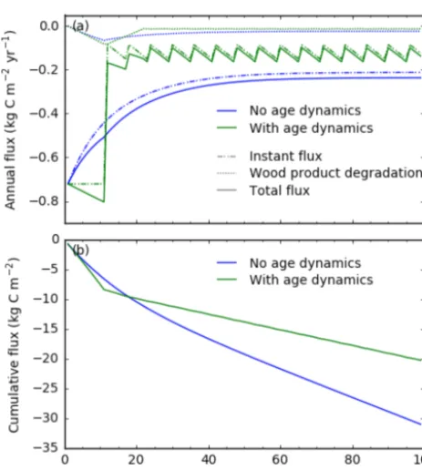
3.1.2 LUC-associated direct carbon fluxes
As shown in Fig. 7a, inSageless, the instantaneous carbon flux
resulting from LUC follows the same temporal pattern as the above-ground biomass, as it is simulated as a fixed frac-tion of above-ground woody mass (sapwood and heartwood) (see Sect. 2.1.5). In Sage, for the initial 12 years, Cohort6
(undisturbed mature forest) is cleared, so that the instanta-neous LUC carbon flux is higher than that inSageless(where
the biomass of the single forest patch is reduced immedi-ately when the land turnover starts). After that, the instanta-neous flux shows a stark drop in Sage when Cohort3enters
the land turnover. Since then until the end of the simulation, Sagekeeps a constantly lower instantaneous flux thanSageless
because the LUC-perturbed equilibrium biomass is higher in the latter case (Fig. 6a). As a fixed 10 % of above-ground woody biomass enters the wood product pool with a 10-year turnover time, delayed carbon emissions from wood prod-uct degradation in both simulations are smaller than the in-stantaneous LUC carbon fluxes. They peak around the 12th year after LUC and remain stable afterwards (Fig. 7a). Over-all,Sagehas a higher LUC-associated direct carbon flux than
Sageless for the first 12 years and a lower one afterwards
(Fig. 7a). The cross point for the cumulative LUC-associated direct fluxes equal inSageandSagelessis around the 20th year
(Fig. 7b). When summing over the whole simulation period (100 years), the cumulative fluxes bySagelessare lower inSage
by about 11 kg C m−2, or∼110 g C m−2yr−1(Fig. 7b) than Sageless.
3.1.3 LUC emission and its disaggregation into underlying component carbon fluxes
As defined in Eq. (4), the net LUC carbon emission (ELUC)
is diagnosed as the difference in NBP between the LUC sim-ulation and the control one. Since NBP is further a compos-ite flux determined by carbon uptake and releases (Eq. 3), the difference inELUC age andELUC ageless can be
disaggre-gated into the effect of each underlying flux, which differs between the LUC simulation and the control simulation. Fig-ure 8 presents such disaggregation. All positive values indi-cate an enhanced carbon uptake or diminished release in the LUC simulation compared to the control one, whereas neg-ative values indicate the reverse cases (i.e. negneg-ative values indicate a contribution to enhanceELUC).
First of all,Sageless (no age dynamics) simulates a larger
magnitude (i.e. a larger absolute ELUC value) of mean
annual ELUC than Sage (with age dynamics) by about
26 g C m−2yr−1. Second, for both simulations, the simulated ELUC is an outcome of LUC-associated direct fluxes being
compensated for by changes in other fluxes, all of which have an effect to reduceELUCin this example: NPP, heterotrophic
some-Figure 7. (a)Carbon fluxes directly associated with LUC (negative values for carbon lost from ecosystems): instantaneous flux (dash-dotted line), flux from wood product degradation ((dash-dotted line), and the total flux (solid line) for simulations with (green) and without (blue) sub-grid age dynamics.(b)Cumulative LUC-associated di-rect fluxes (the sum of instantaneous and wood product degradation fluxes) for simulations with (green) and without (blue) sub-grid age dynamics. Data are shown for an annual forest–cropland turnover of 5 % of the grid cell area for 100 years.
what integrate the effect of recovering young forests or inter-mediately aged forests with a higher productivity than the old-growth forests, as reported by Tang et al. (2014) using observation data.
Averaged over the LUC simulation period of 100 years, both Sage andSageless show lower heterotrophic respiration
(FHR) than the control. This is because the biomass stock is
lower in the LUC simulations (despite a higher NPP, biomass turnover is accelerated due to site perturbation and wood col-lection in the process of clearing forest for cropland), causing less litter input and fewer soil carbon stocks (data not shown). TheSagesimulation shows a much smaller reduction inFHR,
mainly because a higher below-ground litter is maintained, which results from a high below-ground litter input out of land turnover, driven by a high below-ground biomass, as ex-plained in Sect. 3.1.1 (Fig. 6a).
Decreases in fire carbon emissions (FFire, from
prognos-tically simulated natural fires but not land-clearing fires) in the LUC simulations in contrast with the control are be-cause the above-ground litter (dominant fuel for fires) is re-duced by land turnover. Reductions in fire emissions, and reductions in heterotrophic respiration, are thus driven by
Figure 8.Mean annual carbon flux differences between the LUC and control simulations over 100 years for an annual forest– cropland turnover with 5 % of the grid cell area for two model con-figurations: without (blue) and with sub-grid age dynamics (green). Positive (negative) values indicate contributions to enhanced carbon sink (source) in LUC simulation compared to the control one, either by stronger (weaker) carbon uptake or smaller (stronger) carbon re-lease.ELUCis shown as a negative value here, i.e. the LUC simu-lation has a lower NBP than the control one, indicating an effect of net carbon source by LUC.
the same process, i.e. a reduction in above-ground standing biomass. LUC simulations also result in lower agriculture harvest (FAH, from cropland) although there is no change
in the cropland area; this is due to lower biomass in young crop, as the crop harvest is assumed as a constant fraction of the biomass turnover (i.e. routine mortality) at a daily time step. The lower crop biomass in the LUC simulations here is because crop saplings are established on the first day of each calendar year, right before the seasonal biomass peak for the Southern Hemisphere, which artificially reduces the standing biomass.
Overall, the lowerELUCmagnitude inSage is a result of
the lower LUC-associated direct fluxes having been partly compensated for by a higher heterotrophic respiration. The relative magnitudes between ELUC age and ELUC ageless are
dominated by these two fluxes, while other fluxes play a less important role.
3.2 Forest cohort area changes as a result of historical land use change over southern Africa
One of the useful features of our model development is to ac-count for sub-grid forest age dynamics as a result of histori-cal LUC, as illustrated in Fig. 9 for southern Africa. When no LUC is included (S0, the control simulation shown in light blue), the areas of all forest cohorts are constant over time. Except that younger cohorts have a very small area (<0.1 Mkm2) (Cohort2 and Cohort3, probably due to
Figure 9. Areas subject to historical land use change and the resulting modelled temporal changes in areas of different forest cohorts in southern Africa.(a)Areas subjected to historical land use change in which forests are involved. Data are from the LUH1 reconstruction (Hurtt et al., 2011) after adaption for ORCHIDEE-MICT. Three types of LUC activities are shown and their effects elucidated by factorial simulations (Table 4). These are forest loss (blue dashed line) and gain (black dashed line) resulting from net land use change, forest involved in land turnover (both loss and gain in equal amount, green dashed line), and forest area subjected to wood harvest (red dashed line).
(b)–(h)Areas of forest cohorts (Cohort1: the youngest; Cohort6: the oldest) for four factorial simulations (Table 4) in which no land use change occurs in S0, and the three LUC types are added in a factorial set-up in S1 (net land use change, blue solid line), S2 (net land use change+land turnover, green solid line), and S3 (net land use change+land turnover+wood harvest, red solid line). Noteyscale values in
(a)and(h)differ from others.
cells), almost all forests are found in Cohort6, which
resem-bles mature forests. In S1 where only net LUC is considered, the area of Cohort6decreases consistently over time due to
conversion of forest to other land cover types (Fig. 9a). Oc-casional increases in areas of other younger cohorts are also present, corresponding to the periods when forest gain hap-pens due to net LUC, for instance, afforestation or reforesta-tion around the 1700s and in the latter half of the 20th cen-tury (Fig. 9a). This is consistent with our rule that forest from abandonment of agriculture is established in the youngest co-hort (Fig. 5b – on the right), and progressive movement of forests from younger to older cohorts is also visible as the small waves in the curves of Fig. 9b–f.
In the S2 simulation with both net LUC and land turnover, large areas of younger forests, in particular of Cohort1and
Cohort2, begin to appear as a result of continual creation of
forests from land turnover and subsequent moving of forests from Cohort1to Cohort2. Their temporal changes over time
follow those of the forest area subject to land turnover, as
shown in Fig. 9a (green dashed line). The area of Cohort3,
however, does not see as much increase as in the two younger cohorts because forests of Cohort3 are the primary target
for clearance in land turnover and thus are incessantly con-verted back to (shifting) agriculture. As a result, about half of mature forests (Cohort6) are left intact from LUC by 2005
(Fig. 9h). Most interestingly, when there is a decline in the turnover-impacted area around the 1700s (the green arrow in Fig. 9a), a corresponding decline in the area of Cohort1 is
found because these forests move into the next cohort. This pattern of decrease in the current cohort accompanied by the according increase in the next one then propagates into other older cohorts with time, which results in a delayed increase in Cohort5around the 1750s (Fig. 9g), and finally in Cohort6
harvest area only started to rise in the middle of 20th cen-tury, larger areas of Cohort1and Cohort2are found compared
with S2 in the latter half of the last century, and forest area in Cohort6is accordingly lower, being converted to younger
cohorts as a result of harvest.
4 Discussion
DGVMs, either used in an offline mode or coupled with cli-mate models, are powerful tools to investigate the role of past and future LUC in the global carbon cycle perturbed by hu-man activities (Arneth et al., 2017; Le Quéré et al., 2016). Therefore, a more realistic representation of LUC processes in these models is a scientific priority. We included two new features in ORCHIDEE-MICT v8.4.2: gross LUC and forest wood harvest, and sub-grid vegetation cohorts. In a recent review (Prestele et al., 2017), proper representation of gross LUC or sub-grid bidirectional land turnover has been iden-tified as one of the three major challenges in implementing LUC in DGVMs for credible climate assessments, despite that these have already been pioneered by some models (Ta-ble 1). Large underestimation of LUC emissions would occur when gross LUC is ignored, as is shown by several model re-sults reviewed in Arneth et al. (2017).
Shifting cultivation, or forest wood harvest, or more for-est management in general, often involves a stable fallow length or rotation cycle, which involves secondary forests rather than primary ones. In tropical regions, fallow lengths in shifting cultivation range from 10 to 40 years (Bruun et al., 2006; Mertz et al., 2008; Thrupp et al., 1997; van Vliet et al., 2012), with a tendency of reduction in fallow length. In Latin American tropics, agricultural abandonment has al-ready led to prominent growth of secondary forests (Chazdon et al., 2016; Poorter et al., 2016). Forest management, includ-ing wood harvest, is more common in temperate and boreal regions. In European forests, rotation lengths depend on tree species, regional climate, and management purposes, ranging from 8 to 20 years in coppicing systems in southern Europe to 80–120 years in northern countries (McGrath et al., 2015). The prevalence of secondary forests associated with land use and LUC therefore calls for their representation in DGVMs, especially when modelling LUC.
To our knowledge, Shevliakova et al. (2009) performed the first study to include both sub-grid secondary lands and gross transitions in the LM3V model, but the number of PFTs and secondary land tiles are limited in their study (up to in to-tal 12 secondary land tiles compared with 50 in our study). Stocker et al. (2014) included secondary land in LPX-Bern 1.0 but only one tile of secondary land is available. Yang et al. (2010) examined the contribution of secondary forests to terrestrial carbon uptake using the ISAM model by explic-itly including secondary forest PFTs, but they did not in-clude the dynamic clearing of secondary forests nor shift-ing cultivation in LUC. Therefore, none of these studies have
included a dynamic decision rule regarding the ages of co-horts to be targeted in different LUC processes or the possi-bility of targeting different cohort ages in different geograph-ical regions. ORCHIDEE-CAN is especially designed to ad-dress forest management and species change. Although cer-tain LUC such as wood harvest and net land cover changes are included, a more comprehensive LUC scheme addressing gross change is missing (Naudts et al., 2015).
The gross LUC combined with sub-grid cohorts presented here has shown some promising results. We first confirmed that including gross LUC leads to additional carbon emis-sions. However, these additional emissions tend to be overes-timated when secondary forests are not explicitly accounted for. The idealized grid cell simulation explained the mecha-nism driving such overestimation inSagelesssimulations well.
The results presented here are closely linked with our model parameterization and in particular the decision rules regard-ing which forest cohorts to apply for specific LUC processes (Table 2). Land turnover and secondary forest harvest are pa-rameterized to target intermediately aged cohorts as a prior-ity. This is the core mechanism driving the lower LUC emis-sions when sub-grid forest age structure is accounted for.
As a preliminary effort to demonstrate the model be-haviour, the land turnover parameterization is heavily tied with the input LUC forcing data (LUH1), so that the age of Cohort3 (as the primary target for land turnover) is set as ∼15 years, following the assumed mean residence time of shifting cultivation in the LUH1 data set (Hurtt et al., 2011). The model simulations showed that this parameterization is crucial because it largely determines the rotation length in the model and consequently the amount of carbon stocks sub-jected to LUC and the difference in estimated LUC emissions between the two model configurations (SageandSageless). In
this regard it should be noted that the information on rota-tional lengths of shifting cultivation or forest harvest is spa-tially unbalanced and that at present no systematic global compilation exists. The universal setting used in this study is due to the absence of such a compilation. In fact, because the thresholds in woody mass to distinguish forest cohorts could be configured via a spatial map in the model and such maps could vary among different years, and because the primary cohort target is not hard-coded and can be parameterized as well, it is rather straightforward to apply temporally and spa-tially different rotation lengths in the model. Such a feature is well considered in the model development design and could be tested when information on spatially and temporally ex-plicit forest rotation lengths or associated biomass thresholds is available.