www.geosci-model-dev.net/8/2735/2015/ doi:10.5194/gmd-8-2735-2015
© Author(s) 2015. CC Attribution 3.0 License.
OESbathy version 1.0: a method for reconstructing ocean
bathymetry with generalized continental shelf-slope-rise structures
A. Goswami1,a, P. L. Olson1, L. A. Hinnov1,b, and A. Gnanadesikan1
1Department of Earth and Planetary Sciences, Johns Hopkins University, Baltimore, Maryland, USA anow at: Department of Natural Sciences, Northwest Missouri State University, Maryville, Missouri, USA
bnow at: Department of Atmospheric, Oceanic, and Earth Sciences, George Mason University, Fairfax, Virginia, USA Correspondence to: A. Goswami ([email protected])
Received: 12 February 2015 – Published in Geosci. Model Dev. Discuss.: 2 April 2015 Revised: 14 July 2015 – Accepted: 18 July 2015 – Published: 3 September 2015
Abstract. We present a method for reconstructing global ocean bathymetry that combines a standard plate cooling model for the oceanic lithosphere based on the age of the oceanic crust, global oceanic sediment thicknesses, plus gen-eralized shelf-slope-rise structures calibrated at modern ac-tive and passive continental margins. Our motivation is to develop a methodology for reconstructing ocean bathymetry in the geologic past that includes heterogeneous continental margins in addition to abyssal ocean floor. First, the plate cooling model is applied to maps of ocean crustal age to calculate depth to basement. To the depth to basement we add an isostatically adjusted, multicomponent sediment layer constrained by sediment thickness in the modern oceans and marginal seas. A three-parameter continental shelf-slope-rise structure completes the bathymetry reconstruction, extend-ing from the ocean crust to the coastlines. Parameters of the shelf-slope-rise structures at active and passive margins are determined from modern ocean bathymetry at locations where a complete history of seafloor spreading is preserved. This includes the coastal regions of the North, South, and central Atlantic, the Southern Ocean between Australia and Antarctica, and the Pacific Ocean off the west coast of South America. The final products are global maps at 0.1◦×0.1◦ resolution of depth to basement, ocean bathymetry with an isostatically adjusted multicomponent sediment layer, and ocean bathymetry with reconstructed continental shelf-slope-rise structures. Our reconstructed bathymetry agrees with the measured ETOPO1 bathymetry at most passive margins, in-cluding the east coast of North America, north coast of the Arabian Sea, and northeast and southeast coasts of South America. There is disagreement at margins with anomalous continental shelf-slope-rise structures, such as around the Arctic Ocean, the Falkland Islands, and Indonesia.
1 Introduction
Reconstructing paleobathymetry represents a challenge for modeling past climates. The modern ocean bathymetry in-fluences global climate in numerous ways. As examples, the present-day Southern Ocean bathymetry blocks flow through the Drake Passage, which has effects on the magnitude of the circumpolar current (Krupitsky et al., 1996) and the sta-bility of the thermohaline circulation (Sijp and England, 2005). Similarly, in the Northern Hemisphere, variations in the depth of the Greenland–Iceland–Scotland Ridge have been proposed to modulate North Atlantic Deep Water for-mation (Wright and Miller, 1996). On the global scale, tidal dissipation is concentrated in shallow marine environments, while the generation of tides over rough ocean bathymetry has been proposed to play a major role in driving deep ocean mixing (Simmons et al., 2004).
reconstruc-tions of oceans that overly oceanic crust of known age (Xu et al., 2006; Müller et al., 2008a, b; Hayes et al., 2009).
An important element missing from these reconstructions is the shelf-slope-rise region between oceanic crust and con-tinental shoreline. For near-present-day reconstructions, this region can be adapted from modern bathymetry. However, further back in geologic time the structure of the continent– ocean transition becomes increasingly less certain or un-known. Yet this region represents a critical zone for many biological, sedimentary, and oceanographic processes that in-fluence the Earth system.
In this work we develop a method to model shelf-slope-rise structure back through geologic time that is based on modern-day geometric relationships between ocean crust and shoreline, and takes into account the heterogeneity of these compound structures. Modern open ocean bathymetry, a pa-rameterized open ocean sediment thickness and shelf-slope-rise structure are joined together to form a modern ocean bathymetry. We name this reconstructed bathymetry “OES-bathy” (OES: Open Earth Systems; www.openearthsystems. org).
Modern ocean bathymetry reconstructed with this method-ology is used as a test case as it offers the following advan-tages: (1) differences can be assessed between actual ocean bathymetry and the reconstruction; (2) when applied to cou-pled climate models, it can be used to assess the influence of the reconstruction with respect to actual ocean bathymetry; and (3) specific components of the reconstructed bathymetry, e.g., continental shelf-slope-rise structures, can be investi-gated to examine their roles in the Earth system.
2 Data
2.1 Ocean crust age
For the age distribution of the oceanic crust (hereafter “ocean crust age” represented byτ )we use the data from Müller et al. (2008a; who provide global reconstructions of ocean crust age in 1 Ma intervals for the past 140 Ma. For each recon-structed age in Müller et al. (2008a), ocean crust age, depth to basement, and bathymetry are given. The reconstructed bathymetry based on Müller et al. (2008a) is referred to here-after as EB08 (EB: EarthByte). The data are in 0.1◦×0.1◦ resolution (3601 longitude×1801 latitude points). For this project, 000 Ma (modern) crustal age reconstruction data are used (Fig. S1 in the Supplement).
2.2 Modern ocean sediment thickness
We use modern ocean sediment thickness data from Di-vins (2003) and Whittaker et al. (2013). These data are de-rived from seismic profiling of the world’s ocean basins and other sources. The reported thicknesses are calculated us-ing seismic velocity profiles that yield minimum thicknesses. Data values represent the distance between sea floor and
“acoustic basement”. The data are given in 50×50
resolu-tion and have been regridded to 0.1◦×0.1◦resolution values
(Fig. S2) to match the EB08 grid. 2.3 ETOPO1
To construct the shelf-slope-rise structures, ETOPO1 modern bathymetry (Amante and Eakins, 2009) is used. We use the “Bedrock” version of ETOPO1, which is available in a 10×10
resolution (earthmodels.org), regridded to 0.1◦×0.1◦ resolu-tion (Fig. S3) in order to match the EB08 grid (Fig. S1). This version of ETOPO1 includes relief of Earth’s surface depict-ing the bedrock underneath the ice sheets. However, we use only the oceanic points in this data set, so that this has no impact on the reconstructed bathymetry.
3 Methods
Modern ocean basins have different types of crust, including oceanic crust, submerged continental crust, and transitions between these two types. In our reconstruction, the regions underlain by oceanic crust to which an age has been assigned are termed “open ocean” regions. The parts of the ocean basins that occupy the transitional zone between oceanic crust and the emerged continental crust are termed “shelf-slope-rise” regions. These regions typically extend from the boundary of open ocean regions to the coastline. Accord-ingly, the OES ocean bathymetry model involves the merging of open ocean regions and shelf-slope-rise regions (Fig. 1). To accomplish the merging, map-based operations such as computing distances between locations were carried out in ArcGIS 10.1, whereas local calculations such as interpola-tion and statistics were carried out in Matlab R2014a. The workflow is diagrammed in Fig. S9.
3.1 Reconstruction of open ocean regions
Reconstruction of open ocean bathymetry starts with ocean crust age. This information is available only at locations where oceanic crust is preserved or has been reconstructed. The ocean depth to basement is the distance between mean sea level and the top of the basaltic layer of the oceanic crust. Calculation of depth to basement is based on a cooling plate model in which the vertical distance between mean sea level and basementωτ is expressed as
Figure 1. Bathymetric model geometry. (a) Map view showing two
passive continental margins. Section 1 is a standard passive margin, Section 2 is a passive margin with an extended continental shelf. (b) Cross section of the standard passive margin with model geometry.
(c) Cross section of the passive margin with extended continental
shelf model geometry.
Schubert, 2014)
ωd=
−αρm(Tm−Tw)yL (ρm−ρw) " 1 2 − 4 π2 X∞
m=0 1
(1+2m)2exp( −κ
yL2 (1+2m) 2π2τ )
#
, (2)
whereα(3×10⁻⁵K−1)is the volumetric coefficient of ther-mal expansion of the mantle,ρmis (3300 kg m−3)is density of the upper mantle,ρw(1000 kg m−3)is density of sea wa-ter,Tm−Tw(1300 K) is the difference between upper mantle and ocean temperature,κ(3.410835×10⁵m2s−1) is thermal
Table 1. Values forω0andβfrom Crosby et al. (2006) by ocean basin, and percentage of global ocean areas used to calculate weights for the global averages.
Regions % of analyzed ω0 β
ocean (m) (m s−1/2) North Pacific 6.80 % −2821 −315 Eastern Atlantic 3.38 % −2527 −336 Southeastern Atlantic 4.35 % −2444 −347 Global average −2639.80 −329.50
diffusivity, andyL(2619.7 m) is equilibrium plate thickness, all assumed to have constant values.
The equilibrium depth to basementωecorresponds to the limit ofτ → ∞in Eq. (2), appropriate for the oldest crust: ωe=
−αρm(Tm−Tw)yL 2(ρm−ρw)
. (3)
In our reconstruction we use ωe= −5875 m, the mid-point of the range−5750 to−6000 m in the oldest part of the North Pacific (Crosby et al., 2006). We assign an area-weighted average value to the parameterβ (Table 1):
β=2αρm(Tm−Tw)
(ρm−ρw) r
κ
π =329.5 m s
−1
2, (4)
so that κ
yL2
= β√π
2ωe 2
=4.97×10⁻²s−1. (5)
In terms ofωeandβ, Eq. (2) becomes ωd=ωe
1 2
4 π2
X∞
m=0 1 (1+2m)2 exp
−β√π 2ω2
e
(1+2 m)2π2τ
. (6)
We include the first 25 terms in the sum of Eq. (6) to ensure convergence. Lastly, the depth to basement is calculated with Eq. (1).
3.2 Reconstruction of ocean sediment thickness and isostatic correction
Figure 2. Polynomial fit of sediment thickness as a function of ocean crust age using area-corrected global sediment data from Divins (2003)
and Whittaker et al. (2013) (Fig. S2) and age of the underlying oceanic crust from Müller et al. (2008a) (Fig. S1).
Figure 3. OES model sediment thickness based on the sediment thickness parameterization in Fig. 2.
Whittaker et al., 2013) and age of the underlying oceanic crustτ. Sediment loading was calculated using a multicom-ponent sediment layer with varying sediment densities given in Table 2 in 100 m increments of the sediment. The variable sediment densities were calculated from a linear extrapola-tion of sediment densities in Crosby et al. (2006) (Table S1 in the Supplement). For the isostatic correction, in each 100 m sediment layer we calculate an adjusted thickness given by Dz=
100(ρm−ρz) (ρm−ρw)
, (7)
Figure 4. OES model depth to basement calculated using Eqs. (1) and (6) and Table 1 in open ocean regions underlain by ocean crust of
known age.
Figure 5. OES model bathymetry for the open ocean regions with isostatically adjusted multilayer sediment of varying densities shown in
Table 2. The sediment thickness was parameterized as in Fig. 2. The varying sediment densities are from Table 2.
3.3 Reconstruction of shelf-slope-rise structures
To model the shelf-slope-rise structure, profiles from var-ious modern shelf-slope-rise structures at active and pas-sive margin regions from ETOPO1 were examined, along with their corresponding sediment thicknesses taken from Divins (2003). As a representative active margin, the west coast of South America was chosen (Fig. 6). For passive mar-gins, the Atlantic Ocean (north, south and central) and part
of the Southern Ocean were chosen as representative because their complete rifting history is preserved (Figs. 7, S4).
Figure 6. Representative active margin profile off the west coast of South America. (a) Transects (brown lines) drawn by smoothly connecting
transform fault segments using maps by Scotese (2011). Ocean color represents ocean crust age from the PALEOMAP Project (Scotese, 2011). Continents are from the ESRI standard shapefile data library in ArcGIS 10.1. (b) Average profile based on all transects in (a). Light blue line represents mean sea level (m.s.l.), brown points represent sediment thickness obtained from Divins (2003) and dark blue points represent bathymetry from ETOPO1.
Figure 7. Representative passive margin profiles (shelf-slope-rise structure) from the Atlantic and Southern oceans. Ocean colors represent
ocean crust age from the PALEOMAP Project (Scotese, 2011). Continents are from the ESRI standard shapefile data library in ArcGIS 10.1.
(b), (e) and (h). Transects (brown lines) drawn by smoothly connecting transform fault segments using maps by Scotese (2011). (a), (c), (d), (f), (g) and (i): average profiles based on west and east parts of all transects in (b), (e) and (h). Light blue line represents mean sea level,
Table 2. Profile of sediment density vs. depth below sea floor used
in our reconstruction. These sediment densities were calculated from a linear extrapolation of the data in Table S1.
Depth Density of (m) sediment (kg m−3)
0–100 1670
100–200 1740
200–300 1810
300–400 1880
400–500 1950
500–600 2020
600–700 2090
700–800 2160
800–900 2230
900–1000 2300
1000–1100 2370
1100–1200 2440
1200–1300 2510
1300–1400 2580
1400–1500 2650
>1500 2720
ocean. These are derived as
lsh+lsl=M, (8a) lsh+lsl+lr=P , (8b)
lr= −0.290lsl+437.2, (8c)
lsl+lr= −8.28×10⁻³lsh2 +5.486lsh, (8d) whereMandP are the distances of the coastline from points M and P, respectively.
The numerical coefficients in Eq. (8a) and (8d) were ob-tained from fits to ETOPO1 profiles (Figs. 6, 7, S4). In Fig. 8b we plot the width of the slope+rise versus the width of the shelf from a set of passive margin regions that span a range of shelf widths. We then fit a parabola to this data, constraining the parabola to pass through the origin in order to model the structure at active continental margins. We ap-ply this parabolic fit to active margins and to passive margins where the shelf width is less than the parabola maximum, ap-proximately 350 km. Shelves having widths greater than this maximum are treated individually as special cases.
To determine the corresponding depths, we work outward from the coast. First we apply a uniform gradient of 3.2◦in
depth over the width of the shelf. This value of the shelf gra-dient was obtained from analysis of 17 ETOPO1 transects (Fig. S4). For the depth distribution along the slope and rise, we assume another uniform gradient, as illustrated in Fig. 8a, joining the depth at the shelf break with the depth calculated for the open ocean at point P.
This methodology works for all shelf-slope-rise regions except where the shelf is anomalously extended, for example, north of Siberia, the Falkland Islands region, and the complex
Figure 8. Modeling shelf-slope-rise structure as in Fig. 1. (a) The
shelf-slope-rise parameterization shown in a cross section through a passive continental margin. Parameters arelsh, continental shelf width;lsl, continental slope width;lr, rise width;M, maximum ex-tent of oceanic crust (closest to the coastline) from EB08; andP, the boundary between the shelf-slope-rise structure and the open ocean.
regions in Southeast Asia. If the M point is too far from the coastline, so thatlsh+lsl>800 km, or too close to the coast-line, so thatlsh+lsl<100 km, then the relationship among the three widths no longer holds. For these regions we as-sume thatP =M(Fig. 1c). To complete the reconstruction, these regions were filled by interpolation from neighboring regions.
4 Results
4.1 Reconstructed shelf-slope-rise structures
ETOPO1 bathymetry reveals that active margins lack exten-sive shelves (Fig. 6) and their slope gradient is anomalously large. Likewise, sediment thickness profiles show that active margins have little sediment cover near or far from the coast. In particular, sediment thickness on the shelves of active mar-gins rarely exceeds 250 m and gradually thins out beyond the subduction zone towards the open ocean.
In contrast to active margins, passive margins are char-acterized by significant shelf-slope-rise regions. Three out of the 16 passive margin cross sections studied are shown in Fig. 7. The extent of the shelf region varies substantially along passive margin coastlines, which accounts for the scat-ter among the profiles in Fig. 7. For example, in the profile between the southern tips of Africa and South America, the South American side has a very wide, platform-like shelf region that extends for more than 500 km, whereas on the African side the shelf is at most 100 km wide.
The bathymetric gradients at passive continental margin slopes in Fig. S5 vary significantly, from−0.004 to−0.018. Compared to active margins, passive margins are character-ized by greater thickness of sediments and more lateral vari-ability. The greater sediment thickness on passive margins and its greater lateral variability are evident in the 13 passive margin transects shown in Fig. S4.
Figure 8 shows the relationship between the widths of the shelves and the widths of the adjacent slope-rise structure. A transect east–northeast of Newfoundland in the northern part of the Atlantic Ocean (Fig. S4, Set 3, center panel) includes 300 km of continental shelf and nearly 900 km of continen-tal slope-plus-rise structure. The presence of the widely ex-tended Gulf of St. Lawrence may contribute to this anomaly. 4.2 Reconstructed open ocean regions
Our depth-to-basement reconstruction is shown in Fig. 4. The isostatically adjusted, sediment-loaded model bathymetry of the open ocean is shown in Fig. 5, for which only ocean basin areas with ocean crust ages have an assigned bathymetry. The gap between the coastline and open ocean bathymetry is reconstructed with the shelf-slope-rise model described in Sect. 3.3.
The mid-oceanic ridge systems in our open ocean bathymetry in Fig. 4 have an average depth of approximately
−2675 m. Away from the mid-ocean ridges, ocean depth in-creases systematically, and reaches a maximum depth of ap-proximately−5575 m at old crustal ages. In Fig. 5, the open ocean bathymetry is shown with the modeled sediment cover from Fig. 3 isostatically loaded on to it. With this sediment cover added, the bathymetry ranges between −2675 and
−4900 m in the open ocean regions and the maximum depth of the reconstructed bathymetry is approximately−6500 m. The depth range between−4900 and−6500 m is associated with old ocean crust (crustal age in the range ofτ =100– 120 Ma) along the flanks of the Atlantic, Pacific, Southern and Indian oceans, and the Bay of Bengal.
4.3 Model evaluation
The addition of the shelf-slope-rise model completes the OESbathy (Fig. 9), though excluded are ocean islands, seamounts, trenches, plateaus and other localized anomalies plus the underlying dynamical topography. Below we eval-uate the modeled OESbathy with respect to ETOPO1 and EB08.
4.3.1 Statistics
Basic statistics of OESbathy, ETOPO1 and EB08 are summa-rized in Table 3, which highlights major differences among the bathymetries. Compared to the −10 714 m maximum depth of ETOPO1, OESbathy maximum depth is−6522 m, while the deepest point of EB08 is only−5267 m. These dif-ferences from ETOPO1 are due to the absence of trenches in the reconstructions. The average ocean depths for the ETOPO1, OESbathy and EB08 are −3346, −3592 and
−4474 m, respectively, signifying that EB08 in particular is very deep compared to ETOPO1. The standard deviations of the ETOPO1, OESbathy and EB08 are 1772.25, 1668.52 and 785.08 m, respectively. These values suggest that compared to ETOPO1, the EB08 is overall very smooth, whereas OES bathymetry has a variability that is comparable to ETOPO1.
Figure 9. The full OESbathy model including open ocean regions and shelf-slope-rise structures.
Table 3. Statistics of three global ocean bathymetries: ETOPO1 is from Amante and Eakins (2009), EB08 is from Müller et al. (2008a),
and OESbathy is the result of this study. Mean, median, mode, minimum, maximum and standard deviations (SDs) are in meters; skew-ness (measure of horizontal symmetry of data distribution) and kurtosis (tall and sharpskew-ness of the central peak of data distribution) are dimensionless.
Bathymetry Max Min Average Median Mode SD Skewness Kurtosis
OESbathy −6522.17 204.5 −3591.83 −4321.07 −6.22 1668.52 1.34 3.26 ETOPO1 (ocean only) −10714 3933 −3346.41 −3841 −1 1772.25 0.67 2.30 EB08 −5266.97 422.75 −4473.83 −4678.47 −4231.85 785.08 1.81 7.69 ETOPO1–OESbathy 8812.7 −9231.41 242.53 1.43 5.22 1270.46 0.53 5.71 ETOPO1–EB08 9129.19 −6349.64 380.93 151.92 108.01 1009.99 1.22 6.40 OESbathy–EB08 5264.95 −4769.50 216.31 169.99 94.59 921.59 1.31 17.12
4.3.2 Difference maps
To assess the quality of our results, we difference OESbathy from ETOPO1 in Fig. 10, with positive values correspond-ing to regions where OESbathy is deeper than ETOPO1 and negative values corresponding to regions where OESbathy is shallower than ETOPO1. As described in Sect. 3.3, interpo-lations were used in certain regions to complete the recon-struction, for example, the Falkland Island region, north of Siberia, and the complex regions around SE Asia. These re-gions show significant deviations from ETOPO1; in general, OESbathy is much deeper. Some shelf-slope-rise structures are shallower in OESbathy than ETOPO1, such as around the margins of the central Atlantic, whereas in other areas OESbathy is deeper, such as along the east coast of Africa, the Bay of Bengal and the Arctic Ocean margin. Owing to the absence of seamounts and plateaus in OESbathy, those areas display large positive anomalies.
A difference map between the OES sediment thick-ness (Fig. 3) and the Divins (2003) global ocean sediment
Figure 10. ETOPO1 minus OESbathy. In regions with positive values OESbathy is deeper than ETOPO1, and in regions with negative values
OESbathy is shallower than ETOPO1.
4.3.3 Shelf-slope-rise profiles
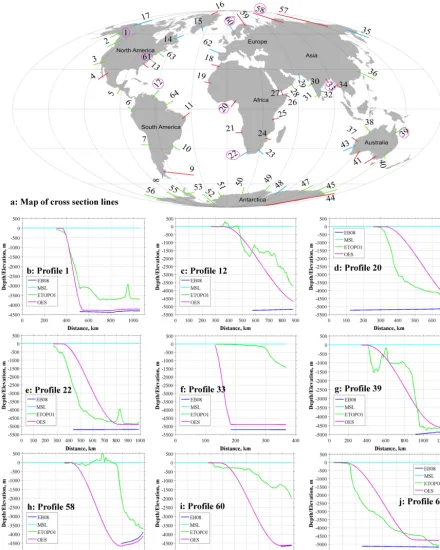
Randomly selected shelf-slope-rise cross sections from all continents, here referred to as “profiles”, are compared for OESbathy, EB08 and ETOPO1 (Figs. 11 and S7). The pro-files shown in Fig. 11b, c, g and j agree well with ETOPO1, while those in Fig. 11d and e are partial fits, and the pro-files in Fig. 11f, h and i are poor fits. In all propro-files, EB08 is shown only for the deep oceans with no continental shelf or slope and as a result none of the EB08 profiles reach the coast. Of the 64 profiles depicted, nearly 50 % fit well with ETOPO1.
Along Profile 1 from the North Pacific (Fig. 11b), OES-bathy is in good agreement with the ETOPO1, especially for the shelf and slope. Beyond 550 km, OESbathy is deeper and lacks the local variations of ETOPO1, such as from the seamounts. EB08 is even deeper than OESbathy along this profile with a similar lack of local variation. Along the north-east coast of South America and Australia (Fig. 11c, g), Pro-files 12 and 39, OESbathy agrees with ETOPO1, whereas the EB08 is deeper than both OESbathy and ETOPO1. Figure 11j shows Profile 61 off the coast of Delaware, USA. Here, there is good agreement between ETOPO1 and OESbathy from the shelf-slope-rise region to the open ocean region out to∼600 km from the coast.
Profiles 20 and 22 (Fig. 11d, e) are taken from coast of Nigeria and the southern tip of Africa. Here, OESbathy has a partial fit with ETOPO1. The OESbathy shelf in both pro-files is wider than ETOPO1 and, as a result, the OESbathy slope+rise is too steep. However, the fit improves in the open ocean along both profiles.
Profiles 58 and 60 (Fig. 11h, i) are from the northern part of Eurasia. This region was filled in by interpolation from nearby regions, because our parameterization fails to model this extremely wide shelf. Hence, along these two profiles there is poor agreement between ETOPO1 and OESbathy. The ETOPO1 shelf is very shallow (<1000 m below sea level), whereas the OESbathy shelf is deeper with a steeper gradient on the slope-rise structure. Similar deviations oc-cur in Profile 33 (Fig. 11f) from the Bay of Bengal, where an enormous pile of sediment from the Ganges system has accu-mulated, resulting in a much shallower ETOPO1 compared to OESbathy.
5 Discussion
5.1 Shelf-slope-rise internal architecture
Figure 11. (a) Location of 61 profiles comparing OESbathy (Fig. 9) with ETOPO1 and EB08. (b–j) Representative profiles at locations
Figure 12. Residual ocean bathymetries. (a) ETOPO1 bathymetry
minus the global oceanic sediment thickness from Divins (2003) with isostatic readjustment applied. (b) The bathymetry from (a) minus the depth-to-basement bathymetry shown in Fig. 4.
Davison and Underhill, 2012). The thickness profiles of the Atlantic margins reflect subsurface graben structures related to the Jurassic–Cretaceous rifting of Pangea (Peron-Pinvidic et al., 2013; Franke, 2013).
The shelf-slope-rise model in Figs. 1 and 8 is based on modern-day bathymetry with three well-defined gradient changes from the coast to the open (deep) ocean. There is no accounting in the model for the complex types of internal architecture in shelf-slope-rise structures just described.
For paleo-ocean reconstructions, extrapolation back through time will produce proportionate narrowing of shelf-slope-rise geometry at passive margins. Highly variable in-ternal structures strongly suggest that simple backward ex-trapolation may not accurately produce paleo-shelf-slope-rise bathymetries, especially for the oldest paleo-oceans. Rifting depends on local lithospheric strength, mantle dy-namics, and global tectonics, all contributing to the evolution of a passive margin in ways that are not easy to parameterize (Ziegler and Cloetingh, 2003; Corti et al., 2004). Thus, addi-tional data such as from seismic profiling and ocean margin drill cores must be consulted before applying these types of corrections for deep time reconstructions.
Lastly, we point out that our shelf-slope-rise formulation constitutes a marked improvement over simple bathymetric
Figure 13. (a) OES model bathymetry minus the global oceanic
sediment thickness from Divins (2003) with isostatic correction ap-plied. (b) The bathymetry from (a) minus the depth-to-basement bathymetry shown in Fig. 4.
interpolation between the coastline and oldest oceanic crust. Bathymetric interpolation would not resolve the extreme dif-ferences in slope between shelf and rise, nor would it faith-fully represent the heterogeneity in shelf lengths found in the modern ocean.
5.2 Residual bathymetry
same sediment correction applied (compare Figs. 12a and 13a). This difference also appears in the residual OESbathy (Fig. 13b), which shows slightly negative mid-ocean ridges, mostly positive coastlines, and very negative terrigenous sed-iment fans.
5.3 Bathymetric impacts on climate
It remains unclear whether the differences between true and reconstructed bathymetry produce qualitatively impor-tant impacts on climate. One fundamental process for which bathymetry is potentially important is ocean tidal amplitude, which depends sensitively on basin resonances (which in turn depend sensitively on the ocean depth affecting the speed of gravity waves; Arbic et al., 2009). As noted above, both lat-eral (Krupitsky et al., 1996) and vertical (Sijp and England, 2005) ocean circulation have also been hypothesized to be sensitive to the details of bathymetry. Work to evaluate these sensitivities in modern models will be a future focus of re-search.
Another key issue concerns reconstructed paleo-bathymetry with simple vertical ocean margins, i.e., no realistic shelf-slope-rise structures, which if applied to oceans could result in substantially inaccurate paleo-climate simulations. The shelf-slope-rise structure is known to present-day ocean models but not for paleo-ocean models; the “modular” aspect of the OESbathy reconstruction provides a convenient means to test the effect of shelf-slope-rise structures on modern climate simulations. Obviously, such a test could be undertaken by simply removing the actual shelf-slope-rise structures from ETOPO1, but to our knowledge this has never been done.
6 Conclusions
The reconstruction method described in this paper was ap-plied to modern data in order to test how well simple param-eterizations of the deep and coastal oceans replicate actual modern ocean bathymetry. Our method uses well-established oceanic crust ages, a cooling plate model, a ized sediment cover for the open oceans, and a parameter-ized shelf-slope-rise structure based on modern bathymetry of ocean margins. The reconstructed bathymetry is called “OESbathy”.
Comparison of OESbathy with ETOPO1 shows global-scale agreement (Fig. 10; Table 3): OES average depth is
−3592±1668 m versus ETOPO1 average depth of−3346±
1772 m, a 7.35 % difference; OES median depth is−4321 m versus ETOPO1 median depth of −3841 m. ETOPO1 is shallower, owing to seamounts and underwater plateaus (LIPs) that are not included in OESbathy. OESbathy max-imum depth is −6522 m versus ETOPO1 maximum depth of −10 714 m, reflecting the absence of a full trench model in OESbathy. Significant differences also occur in complex
coastal regions north of Siberia, the Falkland Islands, and In-donesia.
OES sediment thickness for the open oceans was parame-terized as a multilayer sediment cover, with total thickness based on a third-order polynomial fit between the global ocean sediment thickness data of Divins (2003) and age of the underlying ocean crust. OES sediment thickness fits well to Divins’ sediment thickness in the open oceans, but under-estimates Divins’ sediment thickness at greater ages, espe-cially where terrigenous sediments have accumulated (e.g., Bay of Bengal, Amazon Fan).
The modeled shelf-slope-rise structure for connecting the reconstructed open ocean regions to the continental coast-lines was parameterized with respect to adjacent ocean crust age and present-day geometry of the continental shelf-slope-rise structure. The results show good fits to ETOPO1 for one half of the 64 profiles examined from around the world oceans; the other half of the profiles examined show moder-ate to poor fits to ETOPO1.
Residual ocean bathymetry computed from ETOPO1 con-sistently highlights positive anomalies in the North Atlantic, off the coast of southeast Africa, and the west Pacific Ocean, where actual bathymetry is elevated more than 1.5 km with respect to that produced by a cooling model of the oceanic lithosphere.
The Supplement related to this article is available online at doi:10.5194/gmd-8-2735-2015-supplement.
Acknowledgements. This work is part of the Open Earth Systems
(OES) Project supported by the Frontiers in Earth System Dy-namics Program of the US National Science Foundation, award EAR-1135382. We thank Dietmar Müller (EarthByte) for advice, Christopher R. Scotese (PALEOMAP) for PaleoAtlas data, and Evan Reynolds for technical help throughout the study. We would also like to thank Benjamin Hell and an anonymous referee for their many thoughtful comments that greatly improved our paper.
Edited by: N. Kirchner
References
Amante, C. and Eakins, B. W.: ETOPO1 1 arc-minute global relief model: procedures, data sources and analysis, US Department of Commerce, NOAA, National Environmental Satellite, Data, and Information Service, NGDC, Marine Geology and Geophysics Division, 2009.
Célérier, B.: Paleobathymetry and geodynamics models for subsi-dence, Palaios, 3, 454–463, 1988.
Corti, G., Bonini, M., Conticelli, S., Innocenti, F., Manetti, P., and Sokoutis, D.: Analogue modelling of continental extension: a re-view focused on the relations between the patterns of deforma-tion and the presence of magma, Earth-Sci. Rev., 63, 169–247, 2003.
Crosby, A., McKenzie, D., and Sclater, J.: The relationship between depth, age and gravity in the oceans, Geophys. J. Int., 166, 553– 573, 2006.
Crough, S. T.: The correction for sediment loading on the seafloor, J. Geophys. Res.-Sol. Ea., 88, 6449–6454, 1983.
Davison, I. and Underhill, J. R.: Tectonics and sedimentation in extensional rifts: Implications for petroleum systems, edited by: Gao, D., AAPG Mem. 100, 15–42, 2012.
Divins, D.: NGDC total sediment thickness of the world’s oceans and marginal seas, NOAA, Boulder, CO, 2003.
Franke, D.: Rifting, lithosphere breakup and volcanism: Compar-ison of magma-poor and volcanic rifted margins, Mar. Petrol. Geol., 43, 63–87, 2013.
Hayes, D. E., Zhang, C., and Weissel, R. A.: Modeling paleo-bathymetry in the Southern Ocean, EOS, Transactions, 90, 165– 166, 2009.
Heine, C., Müller, R. D., and Gaina, C.: Reconstructing the lost eastern Tethys ocean basin: convergence history of the SE Asian margin and marine gateways, in: Continent–Ocean Interactions in Southeast Asia, edited by: Clift, P., Kuhnt, W., Wang, P., and Hayes, D., AGU Monograph, 149, 37–54, 2004.
Krupitsky, A., Kamenkovich, V. M., Naik, N., and Cane, M. A.: A Linear Equivalent Barotropic Model of the Antarctic Circumpo-lar Current with Realistic Coastlines and Bottom Topography, J. Phys. Oceanog., 26, 1803–1824, 1996.
Müller, R. D., Roest, W. R., Royer, J.-Y., Gahagan, L. M., and Sclater, J. G.: Digital isochrons of the world’s ocean floor, J. Geo-phys. Res., 102, 3211–3214, 1997.
Müller, R. D., Sdrolias, M., Gaina, C., and Roest, W. R.: Age, spreading rates, and spreading asymmetry of the world’s ocean crust: Geochem. Geophys. Geosys., 9, 1–19, 2008a.
Müller, R. D., Sdrolias, M., Gaina, C., Steinberger, B., and Heine, C.: Long-term sea-level fluctuations driven by ocean basin dy-namics, Science, 319, 1357–1362, 2008b.
Parsons, B. and Sclater, J. G.: An analysis of the variation of ocean floor bathymetry and heat flow with age, J. Geophys. Res., 82, 803–827, 1977.
Peron-Pinvidic, G., Manatschal, G., and Osmundsen, P. T.: Struc-tural comparison of archetypal Atlantic rifted margins: a review of observations and concepts, Mar. Petrol. Geol., 43, 21–47, 2013.
Scotese, C. R.: The PALEOMAP Project Paleo Atlas for ArcGIS, Volume 1, Cenozoic Paleogeographic and Plate Tectonic Recon-structions, PALEOMAP Project, Arlington, Texas, 2011. Sijp, W. and England, M. H.: Role of Drake Passage in controlling
the stability of the ocean’s thermohaline circulation, J. Climate, 18, 1957–1966, 2005.
Simmons, H. L., Jayne, S. R., St. Laurent, L. C., and Weaver, A. J.: Tidally driven mixing in a numerical model of the ocean general circulation, Ocean Model., 6, 245–263, 2004.
Sclater, J. G., Hellinger, S., and Tapscott, C.: The paleobathymetry of the Atlantic Ocean from the Jurassic to the present, J. Geol., 85, 509–552, 1977a.
Sclater, J. G., Abbott, D., and Thiede, J.: Chapter 2: Paleo-bathymetry and sediments of the Indian Ocean, in Indian Ocean Geology and Biostratigraphy, edited by: Heirtzler, J. R., Bolli, H. M., Davies, T. A., Saunders, J. B., and Sclater, J. H., Special Pub-lications, American Geophysical Union, Washington DC, 25–59, 1977b.
Sykes, T. J.: A correction for sediment load upon the ocean floor: Uniform versus varying sediment density estimations – Implica-tions for isostatic correction, Mar. Geol., 133, 35–49, 1996. Turcotte, D. L. and Schubert, G.: Geodynamics, 2nd Edn.,
Cam-bridge University Press, 848 pp., 2014.
Watts, A., Rodger, M., Peirce, C., Greenroyd, C., and Hobbs, R.: Seismic structure, gravity anomalies, and flexure of the Amazon continental margin, NE Brazil, J. Geophys.-Res. Sol. Earth, 114, 1–23, 2009.
Whittaker, J. M., Goncharov, A., Williams, S. E., Müller, R. D., and Leitchenkov, G.: Global sediment thickness data set updated for the Australian-Antarctic Southern Ocean, Geochem. Geophy. Geosys., 14, 3297–3305, 2013.
Wright, J. D. and Miller, K. G.: Control of North Atlantic Deep Wa-ter circulation by the Greenland-Scotland Ridge, Paleoceanogra-phy, 11, 157–170, 1996.
Xu, X. Q., Lithgow-Bertelloni, C., and Conrad, C.P.: Global reconstructions of Cenozoic seafloor ages: Implications for bathymetry and sea level, Earth Planet. Sci. Lett., 243, 552–564, 2006.