www.geosci-model-dev.net/8/1259/2015/ doi:10.5194/gmd-8-1259-2015
© Author(s) 2015. CC Attribution 3.0 License.
A sparse reconstruction method for the estimation of
multi-resolution emission fields via atmospheric inversion
J. Ray1, J. Lee1, V. Yadav2, S. Lefantzi1, A. M. Michalak2, and B. van Bloemen Waanders3
1Sandia National Laboratories, P.O. Box 969, Livermore, CA 94551, USA 2Carnegie Institution for Science, Stanford, CA 94305, USA
3Sandia National Laboratories, P.O. Box 5800, Albuquerque, NM 87185-0751, USA
Correspondence to: J. Ray ([email protected])
Received: 23 July 2014 – Published in Geosci. Model Dev. Discuss.: 20 August 2014 Revised: 7 March 2015 – Accepted: 7 April 2015 – Published: 29 April 2015
Abstract. Atmospheric inversions are frequently used to es-timate fluxes of atmospheric greenhouse gases (e.g., bio-spheric CO2flux fields) at Earth’s surface. These inversions
typically assume that flux departures from a prior model are spatially smoothly varying, which are then modeled using a multi-variate Gaussian. When the field being estimated is spatially rough, multi-variate Gaussian models are difficult to construct and a wavelet-based field model may be more suitable. Unfortunately, such models are very high dimen-sional and are most conveniently used when the estimation method can simultaneously perform data-driven model sim-plification (removal of model parameters that cannot be reli-ably estimated) and fitting. Such sparse reconstruction meth-ods are typically not used in atmospheric inversions. In this work, we devise a sparse reconstruction method, and illus-trate it in an idealized atmospheric inversion problem for the estimation of fossil fuel CO2(ffCO2) emissions in the lower
48 states of the USA.
Our new method is based on stagewise orthogonal match-ing pursuit (StOMP), a method used to reconstruct compres-sively sensed images. Our adaptations bestow three proper-ties to the sparse reconstruction procedure which are useful in atmospheric inversions. We have modified StOMP to in-corporate prior information on the emission field being esti-mated and to enforce non-negativity on the estiesti-mated field. Finally, though based on wavelets, our method allows for the estimation of fields in non-rectangular geometries, e.g., emis-sion fields inside geographical and political boundaries.
Our idealized inversions use a recently developed multi-resolution (i.e., wavelet-based) random field model devel-oped for ffCO2 emissions and synthetic observations of
ffCO2 concentrations from a limited set of measurement
sites. We find that our method for limiting the estimated field within an irregularly shaped region is about a factor of 10 faster than conventional approaches. It also reduces the over-all computational cost by a factor of 2. Further, the sparse reconstruction scheme imposes non-negativity without intro-ducing strong nonlinearities, such as those introduced by em-ploying log-transformed fields, and thus reaps the benefits of simplicity and computational speed that are characteristic of linear inverse problems.
1 Introduction
The estimation of spatially resolved fields, e.g., permeability fields in aquifers or CO2fluxes in the biosphere, from limited
i.e., have few independent parameters, so that they can be estimated from limited observations.
The construction of the spatial parameterization for com-plex fields poses a stiff challenge. The parameterization is usually problem dependent and sometimes based on heuris-tics. One may use an easily observed covariate (or predictor) of the field being estimated to construct such a model; for ex-ample, see Ray et al. (2014) for a description on how images of lights at night were used to create a spatial parameteriza-tion for fossil fuel CO2(ffCO2) emissions. However, one is
never quite sure if the resultant parameterization is too sim-ple or too comsim-plex – in the former case, the estimates will be needlessly inaccurate, while in the latter case, one may not obtain a unique solution or the estimates may reproduce the noise in the observations (overfitting). Consequently, one uses some method, for example, Akaike information crite-rion, to devise models of suitable complexity. However, if the quality of the observations changes with time, then, ide-ally, a different parameterization is constructed for each time instant. In practice, often the simplest model that can be used with all the observations is employed. This degrades estima-tion accuracy.
Sparse reconstruction methods can allow one to circum-vent these problem which arise from the dimensionality of spatial parameterization (also called the random field model). Sparse reconstruction methods such as matching pursuit (MP; Mallat and Zhang, 1993), orthogonal match-ing pursuit (OMP; Tropp and Gilbert, 2007) and Stagewise OMP (StOMP; Donoho et al., 2012) are optimization meth-ods that are used to fit high-dimensional models to lim-ited observations. Unlike other optimization methods, these methods enforce sparsity, i.e., they identify the model param-eters that are not informed by the observations and set them to zero. This is accomplished by augmenting the objective function (usually a `2 norm of the data – model
discrep-ancy or residuals) with a penalty formulated as a `1 norm
over the parameters being estimated. (The`2norm of a
vec-tor x is defined as ||x||2=
q P
ixi2, while the `1 norm is
||x||1=P
i|xi|.) An optimizer is used to manipulate model
parameters to minimize the objective function. The parame-ters that do not impact the residual appreciably are quickly driven to zero, as it minimizes the `1 penalty, i.e., the
op-timizer performs dimensionality reduction while it fits the model to data. This model simplification characteristic of sparse reconstruction methods allows one to dispense with the offline construction of a spatial parameterization and pos-tulate a general, high-dimensional random field model in-stead; thereafter, the optimization method simplifies (reduce the dimensionality of) the random field model in a data-driven manner. In the case of observations with time-variant quality, sparse reconstruction methods have the potential to be particularly useful.
Our interest in sparse reconstruction methods arises from a need to develop accurate spatially resolved estimates of
emissions that are not smoothly distributed in space; ffCO2
emissions are one such example. Estimates of ffCO2
emis-sions are used to assess regional contributions to greenhouse gas emissions and to drive climate change simulations (An-dres et al., 2012). Currently, spatially resolved estimates of ffCO2 emissions are typically derived from national-level
emissions inventories, and are mapped spatially using pop-ulation density or some other proxy of human activity; ex-amples of such spatially resolved inventories are described in Gurney et al. (2009), Olivier et al. (2005), Rayner et al. (2010) and Oda and Maksyutov (2011). Their shortcomings arise from errors in national/provincial reporting and the choice of the proxy used in spatial disaggregation (Andres et al., 2012). Recently, the possibility of using atmospheric observations to constrain fossil fuel emissions, and thereby improve inventories, has been explored (Pacala et al., 2010). Such applications involve the solution of an inverse problem driven by ffCO2concentration measurements (Rayner et al.,
2010). Note that such improvements would be contingent on a good representation of an estimation problem within the context of an inversion, including the use of a suitable param-eterization for the emissions, the characterization of transport model errors, and the availability of an observational network that is sufficient to provide an adequate constraint on ffCO2
emissions; ffCO2emissions for individual urban domes have
been estimated using atmospheric measurements (Turnbull et al., 2011; McKain et al., 2012; Kort et al., 2012), i.e., with-out solving an inverse problem, but existing methods do not offer a scalable approach to updating entire inventories in this manner.
As a step towards enabling such applications, we con-structed a wavelet-based spatial parameterization, called the multiscale random field (MsRF; Ray et al., 2014), to repre-sent ffCO2 emission fields. The MsRF was used to model
ffCO2emissions in the lower 48 states of the USA at 1◦×1◦
spatial resolution. The MsRF covers a rectangular region described by the corners 24.5◦N, 63.5◦W and 87.5◦N, 126.5◦W. The emissions are modeled using Haar wavelets, which provide the sparsest representation of ffCO2emissions
in the relevant region. The model has O(103) independent model parameters which were selected using images of lights at night. Due to its high dimensionality, the MsRF model cannot be used directly given realistic in situ observational limitations. However, a data-driven dimensionality reduction of the MsRF model, using a sparse reconstruction method, could help constrain the inverse problem and make it pos-sible to capture coarse spatial patterns of ffCO2 emissions
(and, perhaps, finer details in the vicinity of the sensors), con-ditioned on atmospheric measurements.
only model rectangular domains; in contrast, the geometry of emission fields could be decided by geographical or political boundaries. (A random field model is a spatial parameteriza-tion for a field defined on a grid. It can be constructed using orthogonal bases such as wavelets; the wavelets’ weights are the model parameters and are treated as random variables. Realizations of these random variables produce a realization of the field. Depending upon the choice of the basis set, e.g., if it contains only a subset of wavelets that can be supported by the grid, the random field model may be able to produce only a subset of the infinite number of fields that the grid can support). Finally, sparse reconstruction methods do not pro-vide a simple mechanism to incorporate prior information or guesses of the field being estimated, a common technique to ensure a unique solution to an inverse problem. This is because methods such as OMP and StOMP were largely de-veloped for the reconstruction of compressively sensed im-ages (Candes and Wakin, 2008) where prior information is weak. In contrast, many emission fields of an anthropogenic nature have inventories that can serve as very informative pri-ors and reconstruction methods could profitably use them.
Our previous work (Ray et al., 2014) focused on the spatial parameterization (the MsRF described above) for estimating ffCO2emission fields via atmospheric inversion. In this
pa-per, we describe the methodological innovations in sparse re-construction techniques that allowed us to perform the inver-sion, despite the high dimensionality of the parameterization. These innovations result in an extension of StOMP which can address the peculiarities of reconstructing an emission field. The StOMP extension will be demonstrated in a top-down inversion, using synthetic observations generated from a known, ground-truth emission field so that we may examine certain algorithmic and numerical aspects of the estimation technique, as described below. The novel algorithmic devel-opments addressed in this paper are
1. Incorporation of a prior model of spatially rough emis-sions: we demonstrate a novel and simple method to in-troduce prior information on spatially rough emission fields (in the form of an approximate field fpr) into StOMP. Currently, sparse reconstruction methods em-ploy no other prior information beyond the phenomeno-logical observation that most fields can be represented quite accurately with a sparse set of judiciously chosen wavelet bases (Candés and Romberg, 2007).
Note, that the term prior model or prior information is used somewhat loosely here since our method is not strictly Bayesian. However, fpr serves a similar func-tion by providing regularizafunc-tion in the inverse problem. 2. Estimating fields in irregularly shaped regions: the MsRF model, being based on wavelets, can only model fields in rectangular domains, whereas our emission field is distributed over an irregular regionR, the lower 48 states of the USA. We demonstrate how this
geomet-rical constraint can be imposed efficiently using random projections, a technique that underlies much of com-pressive sensing. The reconstruction of fields in non-rectangular geometries has no parallel in the compres-sive sensing of images and the method discussed in this paper is the first of its kind.
3. Imposition of non-negativity: the estimation of the emis-sion field is posed as a linear inverse problem (see Sect. 2). Non-negativity of emissions can be enforced by log transforming the field, but converts the problem into a nonlinear one, requiring computationally expen-sive, iterative sparse reconstruction methods, like the one developed in Li and Jafarpour (2010). We develop a simple, iterative post-processing method to enforce non-negativity on the estimated ffCO2 emissions. The
non-negativity enforcement mechanism uses StOMP but does not use the MsRF model. The imposition of non-negativity in the sparse reconstruction of an emis-sion field has never been explored before; for example, in Hirst et al. (2013), the non-negativity constraint was not applied to CH4emissions from landfills.
In this study, we demonstrate our method on an idealized at-mospheric inversion of a spatially rough emission field inR. The method is general, but we use ffCO2as the test case. The
idealizations are enumerated below.
1. We assume that ffCO2can be measured independently
without interference from biospheric CO2fluxes. As
de-scribed in Ray et al. (2014), this could be performed using114CO2(radiocarbon) or other non-CO2tracers,
but the measurement technology is expensive and far from being widely deployable.
2. Inversions require us to adopt a statistical error model for the mismatch between observations and model pre-dictions using the estimated emission field. This er-ror quantifies the aggregate of measurement uncertain-ties and errors introduced by the approximations in the transport model, among others. It varies between mea-surement locations. In this study, we model this mis-match as i.i.d. (independent and identically distributed) Gaussian random variables. We assume a value for the standard deviation of the distribution that is too small compared to what is possible using existing transport models and measurement technologies; further, we use the same error model for all the measurement locations (details in Sect. 4). The small error allowed us to investi-gate the numerical aspects of our formulation and solu-tion algorithms without being substantially affected by observational noise. The small error was also required due to the nature of the measurement network employed in the synthetic data test (see below).
for their locations). This network, sited with biospheric CO2
measurements in mind, has towers which tend to be far from urban areas and thus sources of ffCO2 emissions.
Conse-quently, the modeled ffCO2 concentrations at these towers
tend to be low, forcing us to employ an error model that is unrealistically small. These idealizations lead to limits on the inferences that can be drawn regarding the use of our method in a real-data inversion for ffCO2emission fields; they are
discussed in Sect. 5.
We will estimate the emission field at 1◦×1◦ resolu-tion. Emission fields are averaged over 8 days, and esti-mated over 360 days, i.e., we estimate 360/8=45 fields. ffCO2emission from the Vulcan inventory (version 1) (http://
vulcan.project.asu.edu/index.php; Gurney et al., 2009) serve as the ground truth, to generate the synthetic or pseudo-observationsyobsof time-variant ffCO2concentrations. (The
Vulcan inventory provides hourly ffCO2emissions at 10 km
resolution for the lower 48 states of the USA for 2002; it can also be downloaded at 0.1◦resolution.) The prior model fpr will be constructed using the Emission Database for Global Atmospheric Research (source: European Comission, Joint Research Centre/Netherlands Environmental Assess-ment Agency; Emission Database for Global Atmospheric Research (EDGAR), release version 4.0, http://edgar.jrc.ec. europa.eu, 2009; Olivier et al., 2005), which provides a sin-gle emission field at 1◦resolution for 2005. These choices were driven solely by the easy availability of data.
We evaluate our inversion method using the following metrics. First, we check whether the incorporation of prior information into our modification of the StOMP algorithm improves estimates. Second, we investigate the sparsifying nature of our algorithm. The aim of sparse reconstruction is to estimate parameters supported by data (usually large-scale spatial patterns in the rough emission field) and remove de-tails that are not. We check whether this property of StOMP is retained after our modifications. Finally, we check the ef-ficiency with which our method reconstructs emission fields inside an irregularR. Our use of a wavelet-based spatial pa-rameterization incurs a computational cost which can be lim-ited by a user-defined setting. We check if there is a princi-pled way of computing this setting, e.g., if improvements in results follow a diminishing returns behavior with the com-putational cost.
Note that in this study, we do not use the accuracy of the estimated field as a metric for evaluating our method; we only use estimation accuracy to select between competing formulations of the inverse problem. The estimation accuracy depends on (1) the spatial parameterization (the MsRF) and (2) the information content of the data set, and was explored in detail in our previous paper (Ray et al., 2014). There, we fixed the observational data and used the accuracy of the es-timated emission field to gauge the quality of the MsRF. The converse problem – fixing the MsRF and varying the quantity of data – is not very useful for our StOMP-based algorithm,
since StOMP’s sensitivity to data was addressed in Donoho et al. (2012).
The paper is structured as follows. In Sect. 2, we re-view sparse reconstruction techniques, their use with wavelet models of fields and the tenets of compressive sensing that establish the necessary conditions for successful sparse re-constructions. In Sect. 3, we pose the inverse problem and describe the numerical method used to solve it. Three for-mulations, differing in the manner in which they incorporate fprare examined. In Sect. 4 we perform inversion tests with synthetic data to select the best formulation. We also explain, using the properties required for sparse reconstruction, why the selected formulation performed better than the others. The efficacy of limiting the estimated field withinRusing random projections is also investigated. Conclusions are in Sect. 5.
2 Background
In this section, we review techniques used to estimate CO2
fluxes, compressive sensing and the use of sparse reconstruc-tion in inverse problems.
Estimation of CO2fluxes: let the vectorf be the CO2flux
defined on a grid withNRgrid cells. Letf be of sizeKNR, representing a flux field defined over K time periods. The flux is assumed to be time invariant during a given time pe-riod. The transport of CO2 is modeled as that of a passive
scalar, i.e., the concentration of CO2due tof at an arbitrary
set of sites, is given byy=Hf. Here,y is a vectorKsNs
long,Nsbeing the number of locations where measurements
are collectedKstimes over theKtime periods. The matrix H
(KsNs×KNR) contains the sensitivity of measurements to a CO2source in each grid cell and is computed using an
atmo-spheric transport model such as the Stochastic Time-Inverted Lagrangian Transport Model (STILT; Lin et al., 2003). In an atmospheric inversion, CO2concentrationyobsare measured
at a limited set of locations, usually a set of measurement towers (as in our case) or as column-averaged satellite sound-ings. The measurements are too few or too uninformative to estimatef, with each grid cell treated independently. In case of biospheric fluxes, a prior fluxfpr (with the same dimen-sions asf) can be obtained from a biogeochemical process-based model such as CASA (Carnegie–Ames–Stanford Ap-proach; Potter et al., 1993). The discrepancy (f−fpr) is usually modeled as a multi-variate Gaussian field with co-variance Q (aKNR×KNRmatrix), and the estimation of f is typically performed by minimizing the objective func-tion
J=(yobs−Hf)TR−e1(yobs−Hf)
| {z }
Observation term
+(f−fpr)TQ−1(f−fpr),
| {z }
Prior term
where Re is a diagonal matrix with the data – model
vari-ances and includes many sources of errors including mea-surement errors, aggregation errors and transport model in-accuracies. Methods to solve this linear inverse problem are reviewed in Ciais et al. (2010). A comparison of biogenic CO2fluxes and ffCO2emissions (Fig. 1 in Ray et al., 2014)
shows that ffCO2are multiscale in nature and a multi-variate
Gaussian field approximation of(f−fpr)is unlikely to be accurate. This motivated us to construct the MsRF model for ffCO2emission fields (Ray et al., 2014). The solution of an
inverse problem using MsRF requires the use of a sparse re-construction method that, to date, has been used in the recon-struction of compressively sensed images.
Compressive sensing of images: compressive sens-ing (Romberg, 2008; Candes and Wakin, 2008) is a very effi-cient means of representing images using wavelets. Wavelets are a family of orthogonal bases with compact support that are routinely used to model complex fields, including ffCO2
emissions (Ray et al., 2014). Compact support refers to the fact that a wavelet is defined over a finite region (com-pact support). This is in contrast to other commonly used bases, e.g., sin(kπ x),−∞ ≤x≤ ∞, k∈Z, which have in-finite support. However, like Fourier bases, wavelets are or-thogonal; the scalar product of two different wavelets of the same type and order, e.g., Daubechies wavelets of order 4, is 0. Compressive sensing (CS) is based on two key tenets: compressible representation and encoding via random pro-jections. CS assumes that an image, projected onto a suitable wavelet basis set, will yield wavelet weights (represented by a vectorw) that are mostly very small (i.e., a compressible representation) and can be set to zero. Removing the small wavelets results in a sparse approximation of the image. En-coding via random projections is more involved and deter-mines the necessary conditions for successful sampling. Ran-dom encoding is central to our method for applying boundary conditions, viz., limiting ffCO2 emissions within complex,
non-rectangular boundaries.
Consider an image g of size N, that can be represented sparsely usingLN wavelets. Random encoding, as used in CS, asserts that the image may be sampled by projecting it onto a set of random vectors ψj, to obtain compressive measurementsg0, of sizeN
m,L < NmN:
g0=9g=98w=Aw, (2)
where the rows of the sampling matrix9consist of the ran-dom vectorsψj, the columns of8consist of the orthonormal basis vectors (the wavelets)φi andware the weights (or co-efficients) of the wavelets.8is aN×N matrix while9 is
Nm×N. The bulk of the theory was established in Candes
and Tao (2006), Donoho (2006), Candes et al. (2006) and Baraniuk et al. (2008).
In order that one may recover the original imagegfromg0 using sparse reconstruction, 9 and8must satisfy incoher-ence and a restricted isometry property (Candes and Wakin, 2008). Incoherence implies that no rowψkin9is co-aligned
with column φl in 8 and thus collects information on all bases. It is ensured by choosing some well-known wavelets bases (e.g., Haars or Daubechies 4 and 8) for 8 and ran-dom vectors for9(Tsaig and Donoho, 2006; Coifman et al., 2001). This is formally quantified by the mutual coherence
µ(9,8)of9and8:
µ(9,8)= √
Nmax1≤(k,l)≤N|<ψk,φl>|
= √
Nmax(|Akl|), (3)
whereAklare elements of A. Each row of9 is normalized
to a unit vector. The term|<ψk,φl>|is the projection of rowψk on a wavelet basis φl. Co-alignment of a row ψk0 with a waveletφl0 would lead toAk0l0=1 andAk0l=0 for all l6=l0, indicating that a random vector ψk0 collects in-formation on only one wavelet. The scaling by
√
N is con-ventional. A small mutual coherence ensures that all pro-jections of8on the rows of9 are of moderate magnitude (O(10−1)–O(10−3)). A small mutual coherence aids accu-rate reconstruction. Whenµ(9,8)
√
N, we loosely re-fer to9and8as being incoherent. The restricted isometry property (RIP) is a condition imposed on A which ensures thatwcan be recovered fromg0uniquely without the use of priors (except sparsity). We did not pursue this thread since the use of a prior – making the inventory that suppliesfpr consistent with observations – is the motivation behind this investigation.
Sparse reconstruction of images from compressive mea-surements: the aims of reconstruction in CS are to (1) recover the sparsity pattern (alternatively, identify the components of wthat can be estimated fromg0) and (2) estimate those
ele-ments ofwthat are informed byg0 while setting the rest to
zero. The former can be realized by minimizing the`0norm
ofwwhile the latter is typically achieved by minimizing the
`2norm of the measurement – model discrepancy. However,
an objective function that contains a`0norm is
discontinu-ous, and consequently`0is replaced by an`1norm, which is
more tractable (Donoho et al., 2012). Thus, the optimization problem is posed as
minimize
w∈RN
||w||1, subject to||g0−Aw||2< 2. (4)
Sparsity is sometimes used to solve inverse problems in physics, with the9 operator representing the physical pro-cess. Most of these inverse problems have been in the estima-tion of log-transformed permeability fields (Li and Jafarpour, 2010; Jafarpour, 2013), seismic tomography (Loris et al., 2007; Simons et al., 2011; Gholami and Siahkoohi, 2010) and estimation of point and distributed emissions (Hirst et al., 2013; Martinez-Camara et al., 2013). A more detailed re-view of the sparse reconstruction methods can be found in our previous paper (Ray et al., 2014). Most of these inverse problems involved nonlinear models, i.e., y=a(w), rather thany=Aw, for which incoherence (and RIP) are not well defined and consequently were not investigated.
To summarize, sparse reconstruction techniques and wavelet-based random field models have been used in non-linear inverse problems. In contrast, the problem of estima-tion of spatially rough emission fields is linear, raising the possibilities that (1) the same approach may offer a solution to the emission estimation problem and (2) mutual incoher-ence may provide analytical metrics for the quality of obser-vations and, consequently, solutions. We build on the princi-ples of compressive sensing and sparse reconstruction meth-ods to design an inversion scheme for rough emission fields. In particular, we show (using coherence metrics) why the use offpr was necessary. We also show the degree of computa-tional saving achieved when we use random projections to limit ffCO2emissions withinR.
3 Formulation of the estimation problem
Ray et al. (2014) developed a MsRF model for ffCO2
emis-sions in the USA. The MsRF model allows ffCO2emissions
to be represented asf =8w, where8is a collection of Haar wavelets. Consequently, the observational term in Eq. (1) can be written as ||yobs−H8w||2
2. Compared with Eq. (2), we
see that the transport model H serves as the sampling matrix 9. Since we seek to estimate the wavelet weights w from yobs, an optimization problem like Eq. (4) could be posed with the constraint ||yobs−Aw||2< 2, A=H8. In order
to solve this problem via sparse reconstruction, one requires that H and8be incoherent. As we will show in Sect. 4.2, the incoherence requirement is not met, and sparsity (solely) is not sufficient to solve the problem accurately (as tested in Sect. 4.1). Consequently, we modify StOMP to incorporate a prior emission fieldfpr. We also adapt it to accommodate fields defined over irregularly shaped domains as well as to ensure non-negativity of the estimated field.
Letf be a time-variant, non-negative field defined in an irregular regionR, gridded withNR grid cells. In our case f models ffCO2 emission fields. The field is averaged over
a time periodT and coversKtime periods, i.e., it is a vector
NRKlong.f drives a linear model of observations of ffCO2
concentrations:
yobs=y+=Hf+, (5)
where H is the sensitivity matrix obtained from an atmo-spheric transport model (see Sect. 2), is the model–data mismatch due to measurement and transport model errors andyobsis a vector of time-variant measurements collected
atNsmeasurement towers. Each tower collectsKs
measure-ments over theK time periods, i.e., yobs is a vectorKsNs
long. The H matrix is(KsNs)×(NRK). 3.1 Prior models
We employ two prior models in our work – the MsRF model for ffCO2 emissions and a time-invariant
approx-imation of ffCO2 emissions fpr. The MsRF is a
collec-tion of wavelets and model emissions in the logically rect-angular domain given by the corners 24.5◦N, 63.5◦W and 87.5◦N, 126.5◦W. The MsRF discretizes the domain using a dyadic 2M×2M mesh. Haar wavelets are de-fined on all M levels of this dyadic grid, but not all of them are retained in the MsRF. Wavelets constituting the MsRF model are chosen using radiance-calibrated images of lights at night (http://ngdc.noaa.gov/eog/data/web_data/ v4composites/F152002.v4.tar; Cinzano et al., 2000), which serve as a proxy for human activity and thus capture the spa-tial patterns of ffCO2 emissions. The emission field is
al-lowed to assume non-zero values only withinR, the lower 48 states of the USA. We denote the field during thekth time period asfkand model it as
fk=w0kφ0+
M
X
s=1
X
i,j
ws,i,j,kφs,i,j,
{s, i, j} ∈W(s)=8wk, (6)
whereW(s)contains theLwavelets that constitute the MsRF model, andL is a fraction of the 4M wavelets that can be
supported by a 2M×2M mesh.
The MsRF is also the starting point for developing the sec-ond prior modelfpr. The MsRF provides a sparse represen-tation of the radiances X(s):
X(s)=w(X)0 φ0+X
l,i,j
w(X),l,i,jφl,i,j, {l, i, j} ∈W(s). (7)
X(s) is used to calculate a time-invariant prior model for ffCO2emissions asfpr=cX(s).cis computed such that
Z R
fVdA= Z
R
fprdA=c
Z R
X(s)dA=c
Z R
w(X)0 φ0
+X
l,i,j
w(X),s,i,jφl,i,j
dA,{l, i, j} ∈W(s). (8)
fV in our case is the annually averaged 2005 emission field obtained from EDGAR. The leftmost termR
RfVdA
quan-tifies the total emissions as predicted by EDGAR over R. The term cR
RX(s)dAis an estimate of emissions over the same region but modeled usingfpr. The rightmost term sim-ply replaces X(s)with its wavelet model, in accordance with Eq. (7). The details of how the MsRF and fpr were con-structed are in Ray et al. (2014).fprdiffers from the ground truth (Vulcan emissions aggregated over the lower 48 states) by 5–25 % (see Fig. 9 in Ray et al., 2014).
3.2 Posing and solving the inverse problem
We seek emissions over an entire year (360 days), i.e., we seek F= {f1,f2, . . .fK} = {8w1,8w2, . . .8wK} =e8w. F models the field inR∪R0, whereR0 models the region
outsideR(but inside the rectangular domain modeled by the MsRF) with zero ffCO2emissions. We separate out the fluxes
inRandR0by permuting the rows of
e 8
F =
FR FR0
=
e 8R e 8R0
w,
wheree8Rand8eR0are(NRK)×(LK)and(NR0K)×(LK) matrices, respectively. HereNR0 is the number of grid cells inR0. The modeled concentrations at the measurement
tow-ers, caused byFR, can be written asy=HFR. For arbitrary w,FR0 (the emissions inR0) are not zero andFR0=0 will have to be imposed as a constraint in the inverse problem.
Specifying the constraint in individual grid cells is not very efficient since it leads toNR0Kconstraints. This can get very large in a global inversion at high spatial resolutions. Instead, we adapt an approach from compressive sensing to enforce this constraint approximately. Consider aMcs×(NR0K) ma-trix R, whose rows are direction cosines of random points on the surface of NR0K-dimensional unit sphere. This matrix is called a uniform spherical ensemble (Tsaig and Donoho, 2006). TheMcs projections of the emission fieldFR0 on R, i.e., RFR0, compressively samplesFR0 and setting them to zero during inversion allows us to enforce zero emissions outsideR. In Sect. 4.3, we will investigate the degree of com-putational saving afforded by imposing the FR0 =0 con-straint in this manner. The problem is now modeled as Y =
yobs
0
≈
H8eR R8eR0
w=Gw. (9)
In this equation, G is akin to A in Eq. (2). The left hand side Y is approximately equal to Gwsince the observationsyobs contain measurement errors that cannot be modeled with H.
The case where R0 contains non-zero emissions requires
the use of boundary fluxes and is discussed in Ray et al. (2014).
The wavelet coefficients w in Eq. (9) are not normal-ized and usually display a large range of magnitudes. The wavelets inW(s)at finer scales, i.e., those with a small sup-port, tend to have coefficients with a large magnitude. Their
small support cause the fine-scale wavelets to impact only neighboring measurement towers. In contrast, wavelets at the coarser scales have large footprints that span multiple mea-surement locations. Total emissions inR, as well asyobs, are very sensitive to their coefficients. Solving Eq. (9) as it is in-corporates no information fromfpr beyond the selection of wavelets to be included in8. We explore the incorporation ofe fprin the estimation ofwusing three different approaches:
Approach A: this is the baseline approach and solves Eq. (9) as it is. The lack of normalization ofw, in conjunc-tion with the sparse reconstrucconjunc-tion procedure described be-low, leads to artifacts that will be described in Sect. 4.1.
Approach B: in this formulation, we includefpras a prior. We write the emissions asF=fpr+1F. Substituting into Eq. (9), we getY≈Hfpr+G1w, where1w=w−w(X).
Here,w(X)=c{w(X)0 , w(X),s,i,j}, {s, i, j} ∈W(s), wherecis
obtained from Eq. (8). Simplifying, we get
1Y=Y−Hfpr≈G1w. (10)
Approach C: in approach B we expressed the true fluxFas an additive correction overfpr, thus incorporating the prior information infpr. In approach C, we use the spatial pat-tern offpr, as captured by its wavelet coefficientsw(X), to
normalizew. We rewrite Eq. (9) as Y≈GBB−1w=G0w0= He8
0
R Re80R0 !
w0, (11)
B=cdiag(w(X)), (12)
where w0= {w
s,i,j/(c w(X),s,i,j)},{s, i, j} ∈W(s) are the
wavelet coefficients normalized by those of fpr, e8
0
R= e
8Rdiag(w(X))ande8
0
R0=e8R0 diag(w(X)). Iffpr is close toF, the elements ofw0will be O(1). If fpr is a gross un-derestimate, the elements ofw0will still be of the same order of magnitude, but not O(1). Thus, normalization withw(X)
removes the large differences that exist between the wavelet coefficients at different scales.
In all the three cases, we obtain an underdetermined set of linear equations of the form
ϒ≈0ζ. (13)
HereϒrepresentsY in approaches A and C, and1Y in ap-proach B.0represents G in approaches A and B and G0in approach C.ζrepresentswin approach A,1win approach B andw0in approach C.
Sinceyobsis obtained from a set of locations sited with an eye towards biospheric CO2fluxes (see Ray et al., 2013), it is
unlikely that it will allow the estimation of all the elements of ζ. Further, a priori, we do not know the identity of these un-estimateable elements and so we use sparse reconstruction to find and compute them. Equation (13) is recast similar to Eq. (4):
minimize
ζ∈RN
||ζ||1, subject to ||ϒ−0ζ||2
We solve Eq. (14) using StOMP.||ζ||1is minimized by
set-ting to zero as many elements ofζ as possible, thus enforc-ing sparsity. Meanwhile, the constraint ||ϒ−0ζ||2ensures that the solutions being proposed by the optimization proce-dure provide a good reproduction of the observations. Note ζ contains only the wavelets inW(s). The StOMP algorithm is detailed in Donoho et al. (2012). We will refer to this step in the estimation procedure as step I.
3.3 Enforcing non-negativity onFR
Estimates ofwcalculated by StOMP do not necessarily pro-videFR=e8Rwthat are non-negative. In practice, negative values ofFRoccur in only a few grid cells and are usually small in magnitude. A large fraction of elements ofware set to zero by StOMP. Having identified the sparsity pattern, i.e., the spatial scales that can be estimated fromyobs, we devise an iterative procedure for enforcing non-negativity on FR. We discardFR0 and manipulate the field (the emissions) in
Rdirectly, rather than via the wavelet coefficients.
We seek the non-negative vector E= {Ei}, i=
1. . .Q, Q=(NRK)such that ||yobs−HE||2
||yobs|| 2
≤3. (15)
E is constructed iteratively through a sequenceE1,E2, . . .
EN. E0 is initialized by using the absolute values ofFR calculated by solving Eq. (14). At each iterationm, we seek a correctionξ= {ξi}, i=1. . .Q, where|ξi| ≤1, such that
E(m) =diag(exp(ξ1),exp(ξ2), . . .,exp(ξQ))E(m−1)
≈diag(1+ξ1,1+ξ2, . . .,1+ξQ)E(m−1)
=E(m−1)+1E(m−1),where1E(m−1)=ξTE(m−1).
Since the field must satisfyyobs≈HE(m), we get
yobs−HE(m−1)=1y≈H1E(m−1). (16) This is an underconstrained problem, and we seek the spars-est set of updates 1E(m−1) using StOMP. The corrections are calculated, and the field updated as
ξi=sgn
1Ei(m−1)
E(m)i
!
max 1,
1Ei(m−1)
Ei(m)
!
,
Ei(m)=Ei(m−1)exp(ξi) (17)
to obtainE(m). The convergence requirement in Eq. (15) is
checked withE(m), and if not met, the iteration count is up-datedm:=m+1 and Eq. (16) is solved again.
We will refer to this step in the estimation procedure as step II.
4 Numerical results
In this section, we test the sparse estimation technique in Sect. 3, using synthetic observations. The time periodT over
which the ffCO2emissions are averaged is 8 days.K=45,
i.e., we estimate emissions over 8×45=360 days.Ns=35
towers, which are a subset of NOAA’s Earth System Re-search Laboratory (ESRL) Global Monitoring Division’s co-operative air sampling network (Tans and Conway, 2005); their locations are in Ray et al. (2013). These towers pro-vide continuous observations of CO2concentrations (in parts
per million by volume, ppmv), and 3-hourly averaged syn-thetic observations are used here (i.e.,Ks=24/3×8×45=
2880). We discretize the domain covered by the MsRF us-ing 1◦×1◦grid cells i.e.,M=6. The number of grid cells in the entire domain (the rectangle with the corners 24.5◦N, 63.5◦W and 87.5◦N, 126.5◦W),N, is 4M=4096, which is also equal to the number of wavelets that can be defined on the mesh. The number of wavelets retained in the MsRF,L, is 1031.Rdenotes the lower 48 states of the USA. They are covered withNR=816 grid cells. The number of grid cells outsideR,NR0=N−NR=3280.
The H matrix in Eq. (5) is calculated per the description in Gourdji et al. (2012). We use the Stochastic Time-Inverted Lagrangian Transport Model (Lin et al., 2003), with wind fields from the Weather Research & Forecasting model (Ska-marock and Klemp, 2008), version 2.2, driven by 2008 me-teorology to compute H. Concentration sensitivities are cal-culated at 3 h intervals over a North American grid, at a res-olution of 1◦×1◦. The sensitivity of the CO2concentration
at each observation location due to the flux at each grid cell is calculated in units of ppmv µmol−1m2s1. The sensitivity ofyto the 8-day-averaged emissions were obtained from the 3 h sensitivities by simply adding the 8×24/3=64 sensitiv-ities that span the 8-day period.
The true ffCO2 emissions in R are obtained, for 2002,
from the Vulcan inventory. Hourly Vulcan fluxes are coars-ened from 0.1◦resolution to 1◦, and averaged to 8-day pe-riods. These 8-day-averaged fluxes at 1◦resolution are mul-tiplied by H to obtain ffCO2concentrations at the
measure-ment towers. Note that averaging over 8 days removes the di-urnal variations of ffCO2emissions in Vulcan. Observations
J. Ray et al.: A sparse reconstruction scheme for atmospheric inversion 1267
P
ap
er
|
Discussion
P
ap
er
|
Discussion
P
ap
er
|
Discussion
P
ap
er
|
−120 −110 −100 −90 −80 −70
25 30 35 40 45 50
Longitude
Latitude
EDGAR 2005 emissions; micromoles of C m−2 s−1
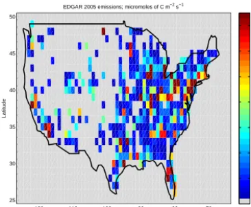
0 0.1 0.2 0.3 0.4 0.5 0.6 0.7
Figure 1.Plot of USffCO2emissions (micromoles of Cm−2s−1) as reported by EDGAR for 2005. Emissions below 0.02 micromoles of Cm−2s−1are grayed out.
34
Figure 1. Plot of ffCO2emissions (micromoles of C m−2s−1) as
reported by EDGAR for 2005. Emissions below 0.02 micromoles
of C m−2s−1are grayed out.
4.1 Comparison of optimization formulations
We choose between approaches A, B and C by solving the inverse problem for the ffCO2emission field. The inversion
is performed for the emissionsF= {fk}, k=1. . .K, for the entire year. The following parameters are used in the inver-sion process:2=10−5, 3=5.0×10⁻⁴, Mcs=13 500, i.e.,
300 random projections for each 8-day period. The rationale for these values can be found in our previous paper (Ray et al., 2014).
In Fig. 2 we plot the estimated emissions during the 31st 8-day period, as calculated using approaches A, B and C. The true emissions are also plotted for reference. Four quadrants are also plotted for easier comparison and reference. The dis-tribution of measurement towers is very uneven, with most of the towers being concentrated in the northeast (NE) quad-rant, where we expect the reconstruction to be most accurate. We see that approach A (Fig. 2, top right) provides estimates that have large areas in the northwest (NW) and southwest (SW) quadrants with moderate levels of ffCO2 emissions.
In contrast, the true emissions (Fig. 2, top left) are mostly empty. Thus, we see that the minimization of||ζ||1 (alterna-tively||w||1) drives the wavelet coefficients to small values,
but not identically to zero. In Fig. 2 (bottom left), approach B provides estimates that show much structure in the eastern quadrants, and the patterns seen infpr(see Ray et al., 2014) are reproduced. The reason is as follows. Whilefprcaptures the broad, coarse-scale patterns of ffCO2emissions, it incurs
significant errors at the finer scales. Equation (10) seeks to rectify the discrepancy between fpr and true emissions us-ing observations. However, as mentioned in Sect. 3.2, fine-scale wavelets tend to have large wavelet coefficients and the minimization of||ζ||1(alternatively||1w||1) removes them since the constraint ||ϒ−0ζ||2
2< 2 is not very sensitive
to individual wavelets at the fine scale. (See Gerbig et al. (2009) for a discussion on the largely local impact of a CO2
flux source.) The inability to rectify the fine-scale discrep-ancies led to a final ffCO2 estimate that resembles fpr in
the finer details. Figure 2 (bottom right) plots the estimates obtained using approach C, which uses normalized wavelet coefficientsw0. The estimates from approach C show large areas of little or no emissions in the western quadrants, sim-ilar to the true emissions in the top-left figure. In the eastern quadrants, the emissions show less spatial structure than the true emissions as well as those obtained using approach A.
The quality of the estimate is due to both the MsRF model and the new sparse reconstruction scheme. The limited ob-servations are sufficient to allow the estimation of the coarse MsRF wavelets, and in certain areas, e.g., the NE quad-rant, finer details. The MsRF model is sufficiently flexible to accommodate the spatial heterogeneity in detail, but re-quires a sparse reconstruction method to address the high di-mensionality that such flexibility entails. Further, the multi-resolution nature of MsRF model allows for the accurate es-timation of coarse-scale patterns of ffCO2 emissions, i.e.,
we expect that aggregate measures of emission quality, such as integrated emissions inR, will be accurate. It will incur larger errors as the domain of integration has shrunk.
In Fig. 3 (top) we evaluate the accuracy of the reconstruc-tion quantitatively. We integrate the emissions inRto obtain the country-level ffCO2emissions and compare that with the
emissions from Vulcan. We plot a time series of errors de-fined as a percentage of total, country-level Vulcan emissions
Errork (%)=
100
K
K
X
k=1
Ek−EV ,k
EV ,k
,
whereEk=
Z R
Ek dAandEV ,k=
Z R
fV ,kdA. (18)
Here,fV ,k are Vulcan emissions averaged over the kth 8-day period andEkare the non-negativity enforced emission
estimates in the same time period. A positive error denotes an overestimation by the inverse problem. In Fig. 3 (bottom) we plot the Pearson correlation coefficient between the true and reconstructed emissions inRover the same duration. We define the Pearson correlation coefficient between Ek and
fV ,kas
C Ek,fV ,k
=cov(Ek,fV ,k)
σEkσfV ,k ,
whereσE2
k andσ
2
fV ,k are the variances of the true and
re-constructed fluxes and cov(Z1, Z2)is the covariance between
two random variablesZ1andZ2. It is clear that approach B
provides the worst reconstructions, with the largest errors and smallest correlations. Approach C tends to over-predict emis-sions a little more than approach A, but has better spatial cor-relation with the Vulcan emissions.
Discussion
P
ap
er
|
Discussion
P
ap
er
|
Discussion
P
ap
er
|
Discussion
P
ap
er
|
−120 −110 −100 −90 −80 −70 25
30 35 40 45 50
Longitude
Latitude
True emissions in 8−day period 31 [micromoles m−2
s−1
]
0 0.1 0.2 0.3 0.4 0.5 0.6 0.7
−120 −110 −100 −90 −80 −70 25
30 35 40 45 50
Longitude
Latitude
Estimated emissions; Approach A
0 0.1 0.2 0.3 0.4 0.5 0.6 0.7
−120 −110 −100 −90 −80 −70 25
30 35 40 45 50
Longitude
Latitude
Estimated emissions; Approach B
0 0.1 0.2 0.3 0.4 0.5 0.6 0.7
−120 −110 −100 −90 −80 −70 25
30 35 40 45 50
Longitude
Latitude
Estimated emissions; Approach C
0 0.1 0.2 0.3 0.4 0.5 0.6 0.7
Figure 2.Plots offfCO2emissions during the 31st 8 day period. The units are micromoles of Cm−2s−1.
Emissions below 0.02 micromoles of Cm−2s−1are grayed out. Top left, we plot true emissions from
the Vulcan inventory. Top right, the estimates from Approach A. Bottom left and right figures contain the estimates obtained from Approaches B and C respectively. Each figure contains the measurement towers as white diamonds. Each figure is also divided into quadrants. We see that Approach A, uncon-strained byfprprovides low levels of (erroneous) emissions in large swathes of the Western quadrants. Approach B reflectsfprvery strongly. Approach C provides a balance between the influence offprand the information inyobs.
35
Figure 2. Plots of ffCO2emissions during the 31st 8-day period. The units are micromoles of C m−2s−1. Emissions below 0.02 micromoles
of C m−2s−1are grayed out. Top left, we plot true emissions from the Vulcan inventory. Top right, the estimates from approach A. Bottom
left and right figures contain the estimates obtained from approaches B and C, respectively. Each figure contains the measurement towers as
white diamonds. Each figure is also divided into quadrants. We see that approach A, unconstrained byfprprovides low levels of (erroneous)
emissions in large swathes of the western quadrants. Approach B reflectsfpr very strongly. Approach C provides a balance between the
influence offprand the information inyobs.
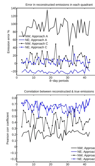
correlation between true and reconstructed emissions (bot-tom) in the northeast (NE) and northwest (NW) quadrants. Errors in the emissions are represented as a percentage of the total (true) emissions in that quadrant. We see the approach C has smaller errors in both the quadrants. It also provides higher correlation in the NW quadrant, which does not have many measurement towers (white diamonds in Fig. 2). Both the approaches have errors of opposite signs in the quadrants which largely cancel out when errors are assessed overRas a whole, leading to approximately similar estimation accura-cies by both the approaches in Fig. 3. However, the estimates produced by approach A (without the use offpr) show larger spatial variability and error than approach C. This is because normalization using w(X) and minimization of||ζ||1
(alter-natively||w0||1) prevents large departures fromfprand also rectifies the tendency to remove large wavelet coefficients be-longing to the finer wavelets. Approach C therefore provides a formulation that is more accurate and robust at the quad-rant scale, even though both have similar fidelity at the scale ofR.
4.2 Evaluating formulation using compressive sensing metrics
Having established empirically that approach A is less accu-rate than approach C, we can explain why this is the case. We employ coherence metrics for this purpose.
In compressive sensing, random matrices such as Gaus-sians, Hadamard, Circulant/Toeplitz or functions such as noiselets (Tsaig and Donoho, 2006; Gan et al., 2008; Yin et al., 2010; Tuma and Hurley, 2009) serve as9. In Fig. 5, we plot the distribution of log10(|Ai,j|), the elements of
A9=98for these standard sampling matrices.8contains
only the wavelets inW(s). Note that max(|Aij|)specifies the
mutual coherence, and small values of max(|Aij|)indicate
informative measurements. We see that log10(|Ai,j|) may
assume continuous (Gaussian and circulant sampling matri-ces) or discrete (Hadamard, scrambled-block Hadamard and noiselets) distributions, and generally lie between −3 and −1. This provides a range for the level of coherence observed in theoretical CS analyses.
oth-J. Ray et al.: A sparse reconstruction scheme for atmospheric inversion Discussion 1269
P
ap
er
|
Discussion
P
ap
er
|
Discussion
P
ap
er
|
Discussion
P
ap
er
|
0 10 20 30 40 50
0 5 10 15 20 25 30 35
Percent error in total emissions
8−day period #
% error in total emissions
Error; Approach A Error; Approach B Error; Approach C
0 10 20 30 40 50
0.55 0.6 0.65 0.7 0.75 0.8 0.85 0.9
Correlation between reconstructed and true emissions
8−day period #
Correlation
Correlation; Approach A Correlation; Approach B Correlation; Approach C
Figure 3.Comparison of estimation error (left) and the correlation between true and estimated emissions
(right) using Approaches A, B and C. It is clear that Approach B is inferior to the others.
36
Figure 3. Comparison of estimation error (top) and the correlation
between true and estimated emissions (bottom) using approaches A, B and C. It is clear that approach B is inferior to the others.
ers. The small values in AH0 indicate that the CO2 concen-tration predictionyat the two selected towers are insensitive to many of the wavelets, i.e., to many scales and locations, as observed in Sect. 4.1. Further, the coherenceµ(H0,8)is larger thanµ(9,8), indicating a sampling efficiency a few orders of magnitude inferior to those achieved in the CS of images. Consequently, approach A, based solely on sparsity, and identical to the method adopted in CS, would not work well. Thus, approach C, which employed both sparsity and fpr, proved superior to approach A.
4.3 Numerical consistency and computational efficiency
We now address some of the numerical aspects of the so-lution. The results presented here are not tests of accuracy of the estimated emission field; estimation accuracy also de-pends on the MsRF and was investigated in Ray et al. (2014). Here we empirically verify that certain necessary conditions of our sparse reconstruction are satisfied.
In Fig. 6 (top), we ploty predicted by the reconstructed emissions at two towers, BAO (Boulder Atmospheric Obser-vatory, Colorado) and MAP (Mary’s Peak, Oregon). These
P
ap
er
|
Discussion
P
ap
er
|
Discussion
P
ap
er
|
Discussion
P
ap
er
|
0 10 20 30 40 50
−20 0 20 40 60 80 100 120 140
8−day periods
Emission error %
Error in reconstructed emissions in each quadrant
NW; Approach A NE; Approach A NW; Approach C NE; Approach C
0 10 20 30 40 50
−0.2 −0.1 0 0.1 0.2 0.3 0.4 0.5 0.6 0.7 0.8
8−day periods
Pearson corr coefficient
Correlation between reconstructed & true emissions
NW; Approach A NE; Approach A NW; Approach C NE; Approach C
Figure 4.
Reconstruction error (left) and correlation between the true and estimated emissions, using
Approaches A and C, for the Northeast (NE) and Northwest (NW) quadrants. We see that Approach C,
which includes information from
f
pr, leads to lower errors in both the quadrants and better correlations
in the less instrumented NW quadrant.
37
Figure 4. Reconstruction error (top) and correlation between the
true and estimated emissions, using approaches A and C, for the northeast (NE) and northwest (NW) quadrants. We see that
ap-proach C, which includes information fromfpr, leads to lower
er-rors in both the quadrants and better correlations in the less instru-mented NW quadrant.
towers were included in the inversion and are not being used as an out-of-sample test of the accuracy of the estimated emission field. Rather, the MsRF for rough fields allows the estimation of local sources which can help reproduce a tower’s measurements very closely, unless neighboring tow-ers provide a constraint; in a sparse network, this is not al-ways possible. Thus, an accurate reproduction of a tower’s observations is not necessarily a sign of an accurately esti-mated emission field, but a bad reproduction can be a sign of a malfunctioning sparse reconstruction method. We see that the ffCO2concentrations are well reproduced by the
1270 J. Ray et al.: A sparse reconstruction scheme for atmospheric inversion
P
ap
er
|
Discussion
P
ap
er
|
Discussion
P
ap
er
|
Discussion
P
ap
er
|
−70 −6 −5 −4 −3 −2 −1 0
0.2 0.4 0.6 0.8 1 1.2 1.4
Distribution of A
i,j from AΨ and AH
Density
log
10(|Ai,j|)
Gaussian Circulant Hadamard sbHadamard Noiselet Tower 2 Tower 21
Figure 5.Comparison of the distribution of the elements ofAΨandAΦ. We see that Gaussian and
cir-culant random matrices lead to continuous distributions whereas Hadamard, scrambled-block Hadamard (sbHadamard) and noiselets serving as sampling matrices lead toAΨ where the elements assume dis-crete values. In contrast, the elements ofAH0 assume values which are spread over a far larger range, some of which are quite close to 1 while others are very close to zero.
38
Figure 5. Comparison of the distribution of the elements of A9
and A8. We see that Gaussian and circulant random matrices lead
to continuous distributions, whereas Hadamard, scrambled-block Hadamard (sbHadamard) and noiselets serving as sampling
matri-ces lead to A9where the elements assume discrete values. In
con-trast, the elements of AH0assume values which are spread over a far
larger range, some of which are quite close to 1 while others are very close to 0.
the range (red symbols in Fig. 6, bottom). During sparse re-construction, these coefficients are set to zero (blue symbols in Fig. 6, bottom). The low-index coefficients, which repre-sent large structures, are estimated accurately. The explicit separation of scales is thus leveraged into omitting fine-scale details which are difficult to inform with data and focusing model-fitting effort on the large scales instead. Sparse re-construction achieves this in an automatic, purely data-driven manner, rather than via a pre-processing, scale-selection step. Finally, we address the issue of enforcing the FR0=0 constraint via random Mcs projections. Naively, the
con-straint can be enforced for every individual grid cell, re-sulting in NR0=3280 linear equations per 8-day period in Eqs. (9) and (13). Considering that yobs=He8R results in 64×35=3240 linear equations per 8-day period, we see that enforcing the constraint is as expensive as computing FR. Instead, we setMcsNR0 random projections ofFR0 to zero in Eqs. (9) and (13), exploiting the basic efficiency-via-random-sampling tenet of CS. Since Eq. (13) is solved approximately, and due to the small number of wavelets in
W(s) that span R0, the constraint F
R0=0 is not satisfied exactly. This error varies with Mcs; a larger Mcs results in
a closer realization of the constraint. Errors in the enforce-ment of theFR0=0 constraint lead to commensurate errors inFR. Here we check the trade-off betweenMcs
(compu-tational efficiency) and accuracy of the estimated emissions (FRandFR0). In practice, this affects only step I of the pro-cedure, where an approximation of ffCO2emissions is
calcu-lated, and thereafter it is used as a guess in step II. However, a good estimate of the emission field accelerates the second step. The quality of the solution from step I, quantified as the
Discussion
P
ap
er
|
Discussion
P
ap
er
|
Discussion
P
ap
er
|
Discussion
P
ap
er
|
0 1 2 3 4 5 6 7 8
−0.2 0 0.2 0.4 0.6 0.8 1 1.2
Days since August 27, 2008
Concentration, ppmv of C
Observed and predicted CO
2 concentrations
BAO; observed BAO; predicted MAP; observed MAP; predicted
100 200 300 400 500 600 700 800 900 1000
−1 −0.8 −0.6 −0.4 −0.2 0 0.2 0.4 0.6 0.8 1
Wavelet coefficient index
tanh(Wavelet coefficient value)
True and estimated wavelet coefficients
True emissions Reconstructed emissions
Figure 6.
Top: predictions of
ffCO
2concentrations at 2 measurement locations, using the true (Vulcan)
and reconstructed emissions (blue lines) over an 8 day period (Period no. 31). Observations occur every
3 h. We see that the concentrations are accurately reproduced by the estimated emissions. Below:
projec-tion of the true and estimated emissions on the wavelet bases for the same period. Coarse wavelets have
lower indices, and they progressively get finer with the index number. We see that the true emissions have
a large number of wavelets with small, but not zero, coefficients. In the reconstruction (plotted in blue),
a number of wavelet coefficients are set to very small values (almost zero) by the sparse reconstruction.
The larger scales are estimated accurately.
39
Figure 6. (Top) predictions of ffCO2concentrations at two
mea-surement locations, using the true (Vulcan) and reconstructed emis-sions (blue lines) over an 8-day period (period no. 31). Observations occur every 3 h. We see that the concentrations are accurately repro-duced by the estimated emissions. (Bottom) Projection of the true and estimated emissions on the wavelet bases for the same period. Coarse wavelets have lower indices, and they progressively get finer with the index number. We see that the true emissions have a large number of wavelets with small, but not zero, coefficients. In the re-construction (plotted in blue), a number of wavelet coefficients are set to very small values (almost zero) by the sparse reconstruction. The larger scales are estimated accurately.
cumulative distribution function of the fluxes can be found in Ray et al. (2013, 2014). There are only a few grid cells with negative emissions and their magnitudes are small.
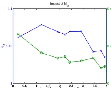
In Fig. 7, we plot the impact ofMcson the reconstruction.
We perform sparse reconstruction of the emission field, for the 31st 8-day period and compute the ratios
ηR=
||fk,R||2
||fV ,k||2 andηR0 =
||fk,R0||2
||fV ,k||2 fork=31, (19) where fk,R and fk,R0 are the emissions over R and R0 from step I. fV ,k is the true (Vulcan) emission field dur-ing the same period. These ratios are plotted as a function of log10(Mcs)per 8-day period. We see that 10 projections
J. Ray et al.: A sparse reconstruction scheme for atmospheric inversion 1271
P
ap
er
|
Discussion
P
ap
er
|
Discussion
P
ap
er
|
Discussion
P
ap
er
|
0 0.5 1 1.5 2 2.5 3 3.5 4
1 1.05 1.1
ηR
log
10(Mcs per 8−day period)
Impact of M
cs
0 0.5 1 1.5 2 2.5 3 3.5 40
0.2 0.4
ηR
′
Figure 7.The impact of the number of compressive samplesMcson the reconstruction ofFR(ηR) and FR0(ηR0).ηRandηR0are plotted on the Y1 and Y2 axes respectively. Results are plotted for the 31st
8 day period. We see thatMcs>103does not result in an appreciable increase in reconstruction quality. Also,Mcs<102shows a marked degradation inηR0.
40
Figure 7. The impact of the number of compressive samplesMcs
on the reconstruction ofFR (ηR) andFR0 (ηR0).ηR andηR0
are plotted on the Y1 and Y2 axes, respectively. Results are plotted
for the 31st 8-day period. We see thatMcs>103does not result in
an appreciable increase in reconstruction quality. Also,Mcs<102
shows a marked degradation inηR0.
period,ηR0 oscillates around 0.1. The corresponding errors infk,Rare about 5 % (ηR≈1.05). In our study we used 300 random projections for each 8-day period. This is about 10 % of the 3280 linear constraints that we would have enforced under a naive implementation of theFR0 =0 constraint. It also halves the computational cost of step I.
5 Conclusions
In this study, we have developed a sparse reconstruction scheme that could be used for solving physics-based lin-ear inverse problems. Our method is an extension of stage-wise orthogonal matching pursuit (StOMP) (Donoho et al., 2012) and borrows many concepts from the compressive sensing (CS) and sparse reconstruction of images (Candes and Wakin, 2008). This scheme is useful for estimating non-stationary fields, e.g., permeability or flux fields, provided their random field model consists of independent parame-ters. This is typically achieved by representing the fields in terms of orthogonal bases, e.g., wavelets or Karhunen–Loève modes, if a prior covariance is available. The dimensionality of the resultant representation is not an issue; the sparse re-construction method estimates only those parameters that are informed by the observations while setting the rest to zero.
Our new method has three novel characteristics. First, it can impose non-negativity on the estimated field, without re-sorting to log transformations. This retains the linear nature of the inverse problem and consequently, its computational efficiency. Second, it allows one to estimate geometrically irregular fields while using a random field model designed for rectangular domains. Third, it allows us to incorporate a prior model of the field being estimated into the sparse construction procedure. While other model-based sparse re-construction methods exist (Baraniuk et al., 2010; He and
Carin, 2009; La and Do, 2005), our method is simple and is seen empirically to recover the correct solution.
We have demonstrated our method in an atmospheric in-verse problem for the estimation of a spatially rough emis-sion field. It is an idealization of the estimation of ffCO2
emissions inR, the lower 48 states of the USA. The emis-sions were modeled in a square domain, with a 64×64 grid, using a recently developed multiscale random field (MsRF) model (Ray et al., 2014). It uses Haar wavelets and images of lights at night to capture the spatial patterns of ffCO2
emis-sion fields. The observational data consists of ffCO2
mea-surements at a limited set of towers, which are linked to the emission field via a CO2 transport model (the forward
model). We draw parallels between our physics-based in-verse problem and the sparse reconstruction of images in CS, and show that a fundamental CS tenet – incoherence – holds only approximately. Consequently, such inverse prob-lems may not bear an accurate solution if they are regularized solely using sparsity. We demonstrate this in our study and show how incorporation of prior information, in the form of spatial patterns in images of lights at night, and a prior model of ffCO2emissions can enable a solution. We also
demon-strate how CS concepts can be used to restrict the estimated field to an irregular region (in our case,R) with a factor-of-ten less computational effort than a naive approach. Finally, we show how non-negativity of ffCO2emissions can be
im-posed using a simple post-processing step.
We also tested whether step I (Sect. 3.2) was necessary by bypassing it completely, and starting step II (Sect. 3.3) with E0initialized using an inventory. We do not present results
of these tests in this paper, but find that the iterative scheme converges only whenE0is very close to the true results. For
example, initializing using perturbed Vulcan emissions led a converged solution, whereasfpr did not. Thus, step I is required for robustness and generality. This is particularly relevant for developing countries where inventories contain larger errors.
Our sparse reconstruction scheme suffers from one serious drawback – it does not provide uncertainty bounds on the estimated field due to the paucity of data, and/or the short-comings of the models. While this can be rectified using a Kalman filter, it does not provide any mechanism for re-ducing the dimensionality of the random field model, should the observational data prove inadequate. This is currently be-ing investigated. Also, we assumed that there were no emis-sions outsideR, but in reality, there are. See our previous pa-per (Ray et al., 2014) on how they could be accommodated as boundary fluxes. Our use of the MsRF in the inversion is a second source of error; in the limit of a very informative mea-surement network, the accuracy of the inversion is limited by the ability of the MsRF to represent ffCO2fields accurately.
Due to the lack of a good tracer for ffCO2 emissions,