Computer-assisted counting of retinal cells by automatic segmentation after TV denoising

Bredieset al. BMC Ophthalmology2013,13:59 http://www.biomedcentral.com/1471-2415/13/59

S O F T W A R E

Open Access

Computer-assisted counting of retinal cells by

automatic segmentation after TV denoising

Kristian Bredies

, Marcus Wagner

, Christian Schubert

and Peter Ahnelt

Abstract

Background: Quantitative evaluation of mosaics of photoreceptors and neurons is essential in studies on development, aging and degeneration of the retina. Manual counting of samples is a time consuming procedure while attempts to automatization are subject to various restrictions from biological and preparation variability leading to both over- and underestimation of cell numbers. Here we present an adaptive algorithm to overcome many of these problems.

Digital micrographs were obtained from cone photoreceptor mosaics visualized by anti-opsin immuno-cytochemistry in retinal wholemounts from a variety of mammalian species including primates. Segmentation of photoreceptors (from background, debris, blood vessels, other cell types) was performed by a procedure based on Rudin-Osher-Fatemi total variation (TV) denoising. Once 3 parameters are manually adjusted based on a sample, similarly structured images can be batch processed. The module is implemented in MATLAB and fully documented online.

Results: The object recognition procedure was tested on samples with a typical range of signal and background variations. We obtained results with error ratios of less than 10% in 16 of 18 samples and a mean error of less than 6% compared to manual counts.

Conclusions: The presented method provides a traceable module for automated acquisition of retinal cell density data. Remaining errors, including addition of background items, splitting or merging of objects might be further reduced by introduction of additional parameters. The module may be integrated into extended environments with features such as 3D-acquisition and recognition.

Keywords: Mammalian photoreceptor cells, Automatical counting, Adaptive algorithm, Continuous optimization, Total variation denoising

Background Introduction

The vertebrate retina contains two or more subtypes of photoreceptors and dozens of interneuron types, thus being organized for effective operation at different light levels and at different bands of the sunlight’s spectrum. Regional shifts in densities and proportions of the sub-types of photoreceptors and interneurons in the retina have been studied intensively as they are assumed to reflect both the evolution of species and specific adapta-tions to their lifestyle [1,2]. Deviaadapta-tions within cell density and mosaic regularity from their normal variability are

*Correspondence: [email protected]

3Center for Physiology and Pharmacology, Medical University Vienna, Schwarzspanierstraße 17, A-1090 Wien, Austria

Full list of author information is available at the end of the article

of specific interest for research involved in developmen-tal control or progressive loss of photoreceptor and other cells due to degenerative diseases and other pathologic processes in the visual system.

Obtaining such data implies the acquisition and ana-lysis of a large number of samples, which is often a time-consuming task requiring persons with appropriate training and experience. Given, moreover, the approx-imately planar organization of retinal layers, the prob-lem of detection and counting of photoreceptor cells is a promising candidate for at least partial automa-tization. However, while various papers have devel-oped options for mapping and analysis of retinal cell mosaic data, once they are digitized [3-7], approaches to full automatization of the time-consuming proce-dure of actual identification and counting have been

rare (we mention [8-10]). Besides the time and com-puting power required for acquiring two- and three-dimensional representations of the tissue of interest, the heterogeneity of the tissue itself is still a major challenge. Many parameters such as tissue thickness/transparency, preparatory and manipulatory distortions change across the retinas, and the cells of interest themselves change in size, shape and spacing. Consequently, for reliable detection of the targets and their differentiation from other items such as debris, other cells, local dam-age or blood vessels highly adaptive algorithms are required.

The present approach focuses on addressing these problems for the segmentation and counting of photore-ceptors. We propose an automatic detection and count-ing procedure, which is based on Rudin-Osher-Fatemi total variation (TV) denoising [11] with subsequent segmentation. As the comparison with manually col-lected data shows, this method is able to detect the targets at comparable reliability. In the view of the authors, the main advantage of the method consists in the complete traceability of all data processing steps and its reproducibility independently from a particu-lar software platform. Thus a possibility for standard-ization and direct comparisons of automatic counts for samples obtained within different environments is provided.

In the present study, the method has been implemented as a MATLAB module and has been applied to single frames (and montages). The method, however, is not lim-ited to the processing of two-dimensional data and can be equally implemented for the analysis of three- or mul-tidimensional data stacks. It could as well be integrated into more comprehensive motorized acquisition setups for stereological sampling or complete mapping of retinal populations.

Retinal image data

Retinal samples from the following species have been

used: Orangutan (Pongo pygmaeus(L. 1760) ), Domestic

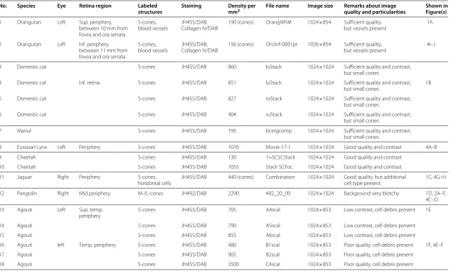
cat (Felis silvestris catus(L. 1758) ), Manul (Felis manul (Pallas 1776) ), Eurasian Lynx (Lynx lynx(L. 1758) ), Chee-tah (Acinonyx jubatus(Schreber 1775) ), Jaguar (Panthera onca(L. 1758) ), Long-tailed Pangolin (Manis tetradactyla (L. 1766) ) and Black-rumped Agouti (Dasyprocta prym-nolopha(Wagler 1831) ) (see Table 1 and Figure 1).

Most of the eyes were obtained from animals delivered to veterinary pathology from zoos and animal parks; some originate from collaborations for other studies [12,13]. Post mortem times were between 0.5 and 12 hours. Eyes were enucleated and immersed in 0.01M phosphate buffer saline (PBS, pH 7.4) with 4% paraformaldehyde. Some were treated after being opened with a cut along the corneal limbus for faster penetration of fixative. Retina

wholemounts were prepared in PBS and flattened by radial cuts, in order to preserve the horizontal and vertical meridian. Cone photoreceptors sensitive to medium/long wavelengths (M-/L-cones) were labeled in isolated Pan-golin retina using JH492 antibody, in all other retinas S-cones were labeled using JH455 (both antibodies pro-vided by J. Nathans [14]). In peripheral Jaguar retina, in addition to S-cones horizontal cells are (unintention-ally) co-labeled by JH455. Retinal vessels in Orangutan were labeled with rabbit anti-mouse collagen IV (AbD Serotec, 2150-1470). After incubation in primary antisera overnight for up to 3 days visualization was done using goat anti-rabbit igg-biotin (Sigma, B7389), ExtrAvidin-peroxidase conjugate (Sigma, E2886) and the diaminoben-zidine (DAB) reaction. After washing in PBS, retinas were gradually transferred up to 90% glycerol, mounted with photoreceptor-side up on a glass slide, and cover slipped.

Manual counting of labeled cones was done within

sampling frames of 150 × 150 μm or 300× 300 μm

using an online-video overlay system consisting of Canvas 5 (ACD Systems, USA) software on a Macintosh com-puter connected with a Hamamatsu 2400 analog came-ra attached to a Nikon Eclipse microscope. This sys-tem allows dual live view of the specimen: through the microscope’s optics or on the video image overlaid by the sampling frames. Optional change of focus and illumina-tion supports optimized online identificaillumina-tion of cells and exclusion of artifacts by position, form, color and other details.

The images (8 or 10 bit grey scale) used for computer-assisted cell counting were obtained by using a Pho-tometrix Camera model CH250/A connected to a Nikon

Eclipse E600 microscope (magnification factors 200×

to 600×) using QED Imaging Software (QED

Imag-ing Inc., Pittsburgh, PA) on a Macintosh computer. In most cases, a projection image (max density or sum) was composed from a stack of images at rele-vant focus levels using the public domain NIH Image program (developed at the U.S. National Institutes of Health; available at http://rsb.info.nih.gov/nih-image/ (accessed 11.02. 2013) ).

Bredies

et

al.

BMC

Ophthalmology

2013,

13

:59

Page

3

o

f

1

3

http://www.biomedcentral.com/1471-2415/13/59

Table 1 Retinal image data

No. Species Eye Retina region Labeled Staining Density per File name Image size Remarks about image Shown in

structures mm2 _{quality and particularities Figure(s)}

1 Orangutan Left Sup. periphery, S-cones, JH455/DAB, 190 (cones) OrangWhM 1024×854 Sufficient quality, 1A between 10 mm from blood vessels Collagen IV/DAB but vessels present

fovea and ora serrata

2 Orangutan Left Inf. periphery, S-cones, JH455/DAB, 156 (cones) OrUinf-0001pr 1026×854 Sufficient quality, 4I–J between 11 mm from blood vessels Collagen IV/DAB but vessels present

fovea and ora serrata

3 Domestic cat S-cones JH455/DAB 860 loStack 1024×1024 Sufficient quality and contrast, but small cones

4 Domestic cat Inf. retina S-cones JH455/DAB 851 luStack 1024×1024 Sufficient quality and contrast, 1B but small cones

5 Domestic cat S-cones JH455/DAB 827 roStack 1024_×1024 Sufficient quality and contrast, but small cones

6 Domestic cat S-cones JH455/DAB 904 ruStack 1024×1024 Sufficient quality and contrast, but small cones

7 Manul S-cones JH455/DAB 195 bcergcomp 1024×1024 Sufficient quality and contrast, but small cones

8 Eurasian Lynx Left Periphery S-cones JH455/DAB 1076 Movie-17-1 1024_×1024 Good quality and contrast 4A–B 9 Cheetah S-cones JH455/DAB 130 1+5CSCStack 1024_×1024 Good quality and contrast

10 Cheetah S-cones JH455/DAB 1055 Stack SCFoc. 1024_×1024 Good quality and contrast

11 Jaguar Right Periphery S-cones, JH455/DAB 440 (cones) Combination 1024×1024 Good quality, but additional 1C, 4G–H horizontal cells cell type present

12 Pangolin Right Mid periphery M-/L-cones JH492/DAB 2290 492_20_09 1024×1024 Background very blotchy 1D, 2A–F, 4C–D 13 Agouti Left Sup. temp. S-cones JH455/DAB 705 A4scal 1024×853 Low contrast, cell debris present 1E

periphery

14 Agouti S-cones JH455/DAB 790 A5scal 1024_×853 Low contrast, cell debris present 15 Agouti S-cones JH455/DAB 855 A6scal 1024×853 Low contrast, cell debris present

16 Agouti left Temp. periphery S-cones JH455/DAB 480 B1scal 1024×853 Poor quality, cell debris present 1F, 4E–F 17 Agouti S-cones JH455/DAB 905 B2scal 1024×853 Poor quality, cell debris present

A

B

C

D

E

F

Figure 1Examples of retinal micrographs used in the experiments.The scale, indicated by the red bar, is 500μm in (A) and 50μm in (B)–(F). (A)Orangutan, No. 1, S-cones and vessels labeled.(B)Domestic cat, No. 4 (clip), S-cones labeled.(C)Jaguar, No. 11 (clip), S-cones and horizontal cells labeled.(D)Pangolin, No. 12 (clip), M-/L-cones labeled.(E)Agouti, No. 13, S-cones labeled.(F)Agouti, No. 16, S-cones labeled. For more details, see Table 1.

Description of the detection and counting method

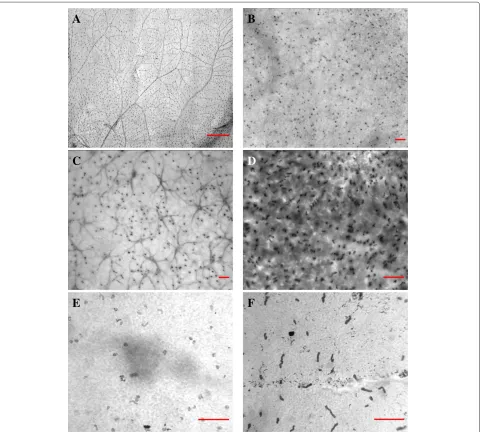
Due to the reasons mentioned in the introduction, the immediate segmentation of the retina image dataI(0) by intensity thresholding leads in many instances to poor results, see below. Therefore, we carry out two process-ing steps before segmentation. In a first step, we generate from the original image I(0)_{, cf. Figure 2A, a}

median-filtered versionIusing window sizemand subtract it from I(0)_{, which results in a considerable removal of}

bright-ness fluctuations in the retinal background, cf. Figure 2B. Subsequently, we subject the image I(0) _{−I = I}(1) _to

a Rudin-Osher-Fatemi TV denoising procedure, cf. [11].

This method, representing a well-established standard in mathematical image processing, may be understood as a kind of filtering, which generates a coarsened, cartoon-like version of the input data, cf. Figure 2C. Nevertheless, during this procedure the images of the dyed retinal cells will be conserved as spots. In mathematical terms, TV denoising means to solve an continuous optimization problem, namely

F(x) =

x(s)−I(1)(s)2ds+α

Bredieset al. BMC Ophthalmology2013,13:59 Page 5 of 13 http://www.biomedcentral.com/1471-2415/13/59

for an unknown functionx(s): →[ 0 , 1 ] , which rep-resents the converted (“filtered”) image. For more details, we refer to the Appendix. Let us only remark that the number α > 0 within (1) remains fixed from the out-set. For the numerical solution of problem (1), surprisingly efficient methods are available by now. In our present study, a recently published solver (by Chambolle/Pock, cf. [15]) has been implemented as a MATLAB subrou-tine. The segmentation of the output x = (xij) of the TV denoising step will be performed now by applica-tion of the following rule: After calculating the expecta-tion E(x) and variance Var(x), we declare all pixels xij with

xij<E(x)−c·Var(x) (2)

as “black enough” to belong to images of photoreceptor cells. Finally, all “black” features consisting of a num-ber of connected adjacent pixels, which is bigger than a given threshold size f, are automatically counted, cf. Figure 2D.

In this method, no more than three parameters remain

to be adjusted manually. These are: the window size m

for the median filter, the parametercin (2), which influ-ences the contrast differentiation between photoreceptor

cells and the background, and the minimal size f of a

connected feature to be recognized as a photoreceptor cell.

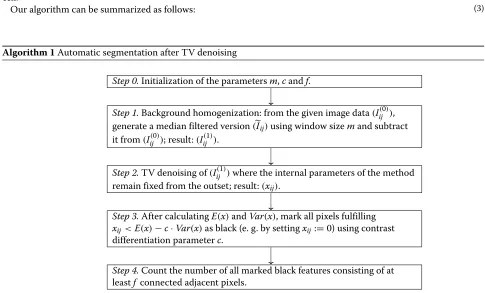
Our algorithm can be summarized as follows:

Implementation

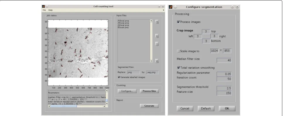
Implementation as a MATLAB tool

Algorithm 1 has been implemented as a MATLAB tool with a graphical user interface (cf. Figure 3A), which allows for batch processing of multiple images. It has been tested on MATLAB 7.14.0.739 (R2012a) and requires the MATLAB Image Processing Toolbox (documented at http://www.mathworks.com/products/ matlab and http://www.mathworks.com/products/image (accessed 11.02.2013) ). In the following, details regard-ing the implementation of the procedure are given. In Step 1, the background homogenization, the median filtering is realized in a straightforward manner by

call-ing the MATLAB procedure medfilt2(image,

[m,m], ’symmetric’) which is part of the image processing toolbox. For the TV denoising in Step 2, the primal-dual algorithm from [15] is

uti-lized. It is realized by performing N steps of the

iteration ⎧ ⎪ ⎪ ⎪ ⎪ ⎪ ⎪ ⎪ ⎪ ⎪ ⎪ ⎪ ⎪ ⎨ ⎪ ⎪ ⎪ ⎪ ⎪ ⎪ ⎪ ⎪ ⎪ ⎪ ⎪ ⎪ ⎩

p(1),k+1 p(2),k+1

=Pα p (1),k

p(2),k

+τ_d

∂_s1+x¯k

∂_s2+x¯k , Pα(v)ij

= α

Maxα,v(_ij1)2+v(_ij2)2

v(_ij1) v(_ij2)

xk+1= 1 1+τp

xk+ τp 1+τp

I(1)+∂_s1−p(1),k+1+∂_s2−p(2),k+1

¯

xk+1=2xk+1− ¯xk

(3)

Algorithm 1Automatic segmentation after TV denoising

Step 0.Initialization of the parametersm,candf.

⏐⏐

Step 1.Background homogenization: from the given image data(I_ij(0)), generate a median filtered version(Iij)using window sizemand subtract it from(I_ij(0)); result:(I_ij(1)).

⏐⏐

Step 2.TV denoising of(I_ij(1))where the internal parameters of the method remain fixed from the outset; result:(xij).

⏐⏐

Step 3.After calculatingE(x)andVar(x), mark all pixels fulfilling xij<E(x)−c·Var(x)as black (e. g. by settingxij:=0) using contrast differentiation parameterc.

⏐⏐

with step sizesτp,τd>0 such thatτp·τd≤0.125 and the forward and backward finite difference operators

∂_s1+x¯k

ij=

¯

xk_i+1,j− ¯xk_ijif 1≤i<n, 0 else ,

∂_s2+x¯k

ij

=

¯ xk

i,j+1− ¯xkijif 1≤j<r, 0 else,

(4)

∂_s1−p(1),k+1

ij= ⎧ ⎪ ⎪ ⎪ ⎨ ⎪ ⎪ ⎪ ⎩

p(₁1_j),k+1 ifi=1 ,

p(_ij1),k+1−p_i(₋1)_1,,k_j+1if 1<i<n,

−p_n(1₋),_1,k+_j1 ifi=n,

(5)

∂_s2−p(2),k+1

ij= ⎧ ⎪ ⎪ ⎪ ⎨ ⎪ ⎪ ⎪ ⎩

p(_i12),k+1 ifj=1 ,

p(_ij2),k+1−p(_i,2_j−),k₁+1if 1<j<r,

−p_i(2_,r)₋,k₁+1 ifj=r.

(6)

The initializations arex0_{= ¯x}0_=I(1)_,p(1),0_=p(2),0_=0,

and the output will be given by(xij) = (xNij). As default values of the regularization parameter and the number

of iterations, we use α = 0.05 and N = 50. Note

that, in principle, other minimization algorithms could be implemented for solving the TV denoising problem. For

A

B

C

D

E

F

Bredieset al. BMC Ophthalmology2013,13:59 Page 7 of 13 http://www.biomedcentral.com/1471-2415/13/59

Figure 3Screenshots of the MATLAB software tool.(A)Main graphical user interface.(B)The configuration dialog.

instance, we mention the generalized TV approach from [16] and the optimal control method described in [17], which is based on the interior-point solver IPOPT [18,19]. The thresholding in Step 3 is realized with the help of

the built-in MATLAB functionsmeanand var. Finally,

for Step 4, the labelling and counting procedure, the func-tionbwlabelis utilized, which is again part of the image processing toolbox. It yields a labelled image in which each connected component is identified by a positive inte-ger. With this information, the identification and counting of those connected components, which comprise at leastf pixels, can be easily realized.

Usage

Usually, in order to analyze the topography of items in a retina preparation, a considerable number of image files has to be generated, each showing a segment. Our soft-ware tool was especially designed to cope with multiple files showing similar structures. In this situation, it is pos-sible to start with a manual count within one or two typical images in order to calibrate the parametersm,candf. This can be done by starting the program and adding a single image to the file list. In most cases, the default param-eters give a good starting point, hence one can perform a segmentation in order to decide whether one is satis-fied with the results. Otherwise, adjust the parametersm, candf using the configuration dialog (cf. Figure 3B) and try again. Once the parameters have been adjusted, they can be utilized for the analysis of the whole image set. The batch processing feature of the software allows to per-form this analysis without further user interaction: simply add the remaining files to the list and start the segmenta-tion procedure. Finally, a report which lists, for each file in the batch, the number and mean density of detected

cells as well as their positions, can be automatically gen-erated. As default values for the parameters m, candf,

we encodedm = 30,c = 2.5 and f = 5. Eventually,

for convenience and reproducibility, the tool also provides saving and loading of the file list as well as of a list of all parameters.

Results and discussion

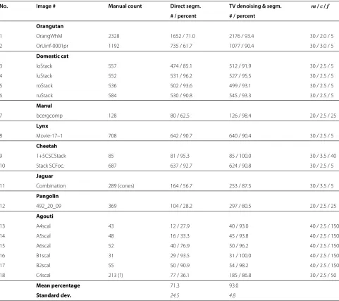
The results of automatical counting are documented in Tables 2, 3 and 4. In order to justify the application of a counting procedure, it is essential that manually counted data are reliably matched. Consequently, the counts generated by TV denoising and subsequent seg-mentation are compared with carefully realized manual counts. The results are listed in Table 2. Furthermore, for every automatic count the number of recognized cells, which have also been marked in the manual counting procedure (Table 3), as well as the number of artifacts (Table 4) were identified. For comparison, we performed automatic counts by direct segmentation without preced-ing TV denoispreced-ing uspreced-ing the same parameterscandf as in Algorithm 1.

Table 2 Overall cell counts by different methods

No. Image Manual count # Direct segm. TV denoising & segm. m/c/f

# / rel. error # / rel. error

Orangutan

1 OrangWhM 2328 1784 / 24.9 2286 / 1.8 30 / 2.0 / 5

2 OrUinf-0001pr 1192 793 / 33.5 1168 / 2.0 30 / 3.0 / 5

Domestic cat

3 loStack 557 518 / 7.0 543 / 2.5 30 / 2.5 / 5

4 luStack 552 584 / 5.8 562 / 1.8 30 / 2.5 / 5

5 roStack 536 539 / 0.6 520 / 3.0 30 / 2.5 / 5

6 ruStack 584 573 / 1.9 573 / 1.9 30 / 2.5 / 5

Manul

7 bcergcomp 128 110 / 14.1 128 / 0.0 20 / 2.5 / 25

Lynx

8 Movie-17-1 708 675 / 4.7 659 / 6.9 30 / 2.5 / 5

Cheetah

9 1+5CSCStack 85 84 / 1.2 91 / 7.1 30 / 3.5 / 40

10 Stack SCFoc. 687 656 / 4.5 634 / 7.7 30 / 2.5 / 5

Jaguar

11 Combination 289 (S-cones) 177 / 38.8 275 / 4.8 30 / 3.5 / 5

Pangolin

12 492_20_09 369 109 / 70.5 367 / 0.5 20 / 2.5 / 25

Agouti

13 A4scal 43 14 / 67.4 44 / 2.3 40 / 2.5 / 150

14 A5scal 48 20 / 58.3 54 / 12.5 40 / 2.5 / 150

15 A6scal 52 44 / 15.4 53 / 1.9 40 / 2.5 / 150

16 B1scal 31 35 / 12.9 43 / 38.7 40 / 2.5 / 150

17 B2scal 55 51 / 7.3 56 / 1.8 40 / 2.5 / 150

18 C4scal 213 (?) 95 / 55.4 234 / 9.8 30 / 2.5 / 50

Mean error 23.6 5.9

Standard dev. 23.6 8.6

Within Algorithm 1, the following parameters have been chosen: The median is taken over a field ofm×mpixels, the TV denoising procedure is applied with regularization parameterα₌0.05and 50 iterations, the contrast differentiation parameter isc, and the minimal size of a recognized feature isfpixels. For comparison, a direct segmentation of the images has been performed as well, applying Steps 3 and 4 of Algorithm 1 with the same values ofcandfdirectly to the image data. Together with the automatic counts, their accuracy is given in terms of the relative error (in percents) related to the manual counts from the third column.

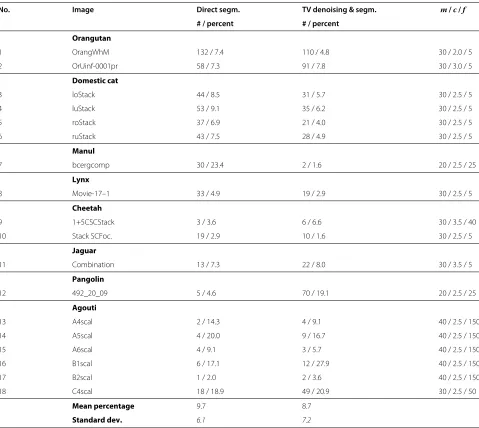
than 90% of the manually marked cells in 15 of 18 cases (93.0% in the mean). The number of artifacts contained in the counts, as listed in Table 4, amounts to 8.7% in the mean. Thus, given that the TV/segmentation method makes no use of additional information about the shape of the cells or the variation of their size, these results are quite satisfactory.

As to be expected, our results show that automatic counting by the TV/segmentation method is superior to direct segmentation in every respect. The mean relative error produced by the latter amounts to as much as 23.6%, and the relative error goes below 10% in 8 of 18 cases only. The loss of precision is mostly caused by the fact that,

by direct segmentation, a significantly smaller number of marked cells is recognized than by the TV/segmentation method (cf. Figure 2D–F) while the ratio of artifacts pro-duced by both methods is comparable. The superiority of the TV/segmentation method can be seen as well by com-paring the standard deviations of the indicators. Let us remark that, during our experiments, we further observed that the TV/segmentation method is even superior to direct segmentation after subtraction of the median (Steps 1, 3 and 4 of Algorithm 1).

Bredieset al. BMC Ophthalmology2013,13:59 Page 9 of 13 http://www.biomedcentral.com/1471-2415/13/59

Table 3 Number of correctly recognized cells within the automatic counts

No. Image # Manual count Direct segm. TV denoising & segm. m/c/f

# / percent # / percent

Orangutan

1 OrangWhM 2328 1652 / 71.0 2176 / 93.4 30 / 2.0 / 5

2 OrUinf-0001pr 1192 735 / 61.7 1077 / 90.4 30 / 3.0 / 5

Domestic cat

3 loStack 557 474 / 85.1 512 / 91.9 30 / 2.5 / 5

4 luStack 552 531 / 96.2 527 / 95.5 30 / 2.5 / 5

5 roStack 536 502 / 93.6 499 / 93.1 30 / 2.5 / 5

6 ruStack 584 530 / 90.8 545 / 93.3 30 / 2.5 / 5

Manul

7 bcergcomp 128 80 / 62.5 126 / 98.4 20 / 2.5 / 25

Lynx

8 Movie-17–1 708 642 / 90.7 640 / 90.4 30 / 2.5 / 5

Cheetah

9 1+5CSCStack 85 81 / 95.3 85 / 100.0 30 / 3.5 / 40

10 Stack SCFoc. 687 637 / 92.7 624 / 90.8 30 / 2.5 / 5

Jaguar

11 Combination 289 (cones) 164 / 56.7 253 / 87.5 30 / 3.5 / 5

Pangolin

12 492_20_09 369 104 / 28.2 297 / 80.5 20 / 2.5 / 25

Agouti

13 A4scal 43 12 / 27.9 40 / 93.0 40 / 2.5 / 150

14 A5scal 48 16 / 33.3 45 / 93.8 40 / 2.5 / 150

15 A6scal 52 40 / 76.9 50 / 96.2 40 / 2.5 / 150

16 B1scal 31 29 / 93.5 31 / 100.0 40 / 2.5 / 150

17 B2scal 55 50 / 90.9 54 / 98.2 40 / 2.5 / 150

18 C4scal 213 (?) 77 / 36.1 185 / 86.8 30 / 2.5 / 50

Mean percentage 71.3 93.0

Standard dev. 24.5 4.8

The percentages are given in relation to the manual counts in the third column.

Let us briefly compare the proposed method with other approaches pursued in the literature. In [8], the authors perform the image processing steps by use of a commer-cial software package which, unfortunately, comes as a “black box” without documentation of the internally uti-lized algorithms. In [9,10,20,21], after certain presmooth-ing/denoising steps, watershed segmentation is employed. Additionally, before segmenting, in [20] an illumination correction is performed while the authors in [10] inter-pose a contrast enhancement step. A common feature of all approaches is the necessity to select a number of parameters, including the (expected or minimal) feature size, by the experimenter.

Although preprocessing steps, particularly denoising or smoothing of the raw image data, are crucial for the

quality of the results of subsequent segmentation, they have not been thoroughly documented in the cited ref-erences (if at all), and their dependence on additional, manually tuned parameters remains unclear. Moreover, any denoising method generates artifacts, thus modifying fine structures within the images in a specific way. In con-trast to this situation, the preprocessing steps involved in our method (median filtering and TV denoising) are traceable and reproducible, including the manual

set-ting of the single parameter m. For the TV denoising

Table 4 Artifacts within the automatic counts produced by the different methods

No. Image Direct segm. TV denoising & segm. m/c/f

# / percent # / percent

Orangutan

1 OrangWhM 132 / 7.4 110 / 4.8 30 / 2.0 / 5

2 OrUinf-0001pr 58 / 7.3 91 / 7.8 30 / 3.0 / 5

Domestic cat

3 loStack 44 / 8.5 31 / 5.7 30 / 2.5 / 5

4 luStack 53 / 9.1 35 / 6.2 30 / 2.5 / 5

5 roStack 37 / 6.9 21 / 4.0 30 / 2.5 / 5

6 ruStack 43 / 7.5 28 / 4.9 30 / 2.5 / 5

Manul

7 bcergcomp 30 / 23.4 2 / 1.6 20 / 2.5 / 25

Lynx

8 Movie-17–1 33 / 4.9 19 / 2.9 30 / 2.5 / 5

Cheetah

9 1+5CSCStack 3 / 3.6 6 / 6.6 30 / 3.5 / 40

10 Stack SCFoc. 19 / 2.9 10 / 1.6 30 / 2.5 / 5

Jaguar

11 Combination 13 / 7.3 22 / 8.0 30 / 3.5 / 5

Pangolin

12 492_20_09 5 / 4.6 70 / 19.1 20 / 2.5 / 25

Agouti

13 A4scal 2 / 14.3 4 / 9.1 40 / 2.5 / 150

14 A5scal 4 / 20.0 9 / 16.7 40 / 2.5 / 150

15 A6scal 4 / 9.1 3 / 5.7 40 / 2.5 / 150

16 B1scal 6 / 17.1 12 / 27.9 40 / 2.5 / 150

17 B2scal 1 / 2.0 2 / 3.6 40 / 2.5 / 150

18 C4scal 18 / 18.9 49 / 20.9 30 / 2.5 / 50

Mean percentage 9.7 8.7

Standard dev. 6.1 7.2

The percentages are given in relation to the corresponding counts from columns 4 and 5 in Table 2.

instead of watershedding. The latter approach is well suited for the analysis of large, clumpy cell aggregates while our method is better suited for the detection of sin-gle cells to be differentiated from a more or less blotchy background, which may contain additional structures like vessels or different cell types. The segmentation depends

on no more than two further parameters candf, which

have to be selected on the base of the observed contrast as well as of a reasonable guess of the feature size. A possible improvement could be the introduction of an additional upper bound for the size of the recognized features, thus reducing and possibly underestimating the number of cells since larger aggregates formed of merged cell images will then be excluded.

The reliability of our method, when evaluated by the mean relative error of automatic counting in relation to manual counts (5.9% as documented above), fits well within the range of errors documented in the cited

ref-erences: [9], p. 1969, Figure one: ≤ 10% in 11 of 23

cases; [10], p. 641, Figure two: ≤ 5% in 31 of 40 cases; [20], p. R100.7, Figure two(A): 6% and 17%; [21], p. 589, Figure three:≤10% in roughly half of the cases.

Bredieset al. BMC Ophthalmology2013,13:59 Page 11 of 13 http://www.biomedcentral.com/1471-2415/13/59

data stacks. Concerning the runtime behaviour, the anal-ysis of an 1024×1024-pixel image takes typically less than 40 sec (on a Mini-PC equipped with four proces-sors Intel(R)Core(TM)i3 CPU M380 @ 2.53 GHz) where approximately half of the time is consumed by the median filtering procedure. No particular attempts for tuning have been made.

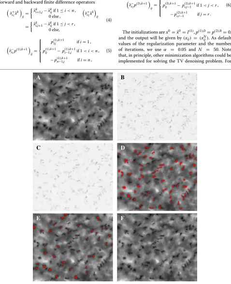
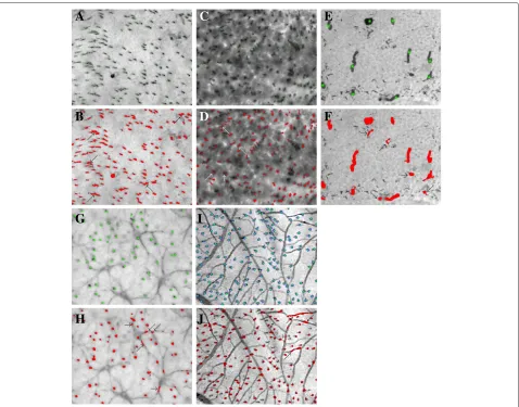
The limitations of the proposed method are exemplified in Figure 4. It shows typical errors within the automatic counting, which would be avoided by a human examiner. Adjacent cells are merged and counted as a single feature (Figure 4A and B). Another typical error occurs when a single photoreceptor cell does not lie exactly in the image plane. The resulting blurred image, may be “broken” into

two or more features, resulting in double or multiple counts (Figure 4C and D). Also, cell debris and back-ground spots may not be recognized as such (Figure 4E and F). Consequently, for heavily contaminated samples such as Nos. 16 and 18, a reduction of the quality of the automatic count is to be expected (in Table 2, No. 16 is the outlier). If background structures such as horizontal cells or vessels are present in the samples, it may happen that parts of them will be counted for cells as well (Figure 4G– J). Normally, however, the TV denoising method is well able to differentiate horizontal cells or vessels and even to recognize target cells, which are positioned immedi-ately above a horizontal cell or a vessel. This is exemplarily shown in Figure 4G–J as well.

A

B

G

H

I

J

C

D

E

F

Conclusions

In conclusion, the presented approach provides a repro-ducible method for the segmentation of labeled cellular objects, in particular retinal photoreceptors from grey scale micrographs. Relatively simple outlines and little overlap between the targets in the projection plane are clearly important preconditions for the current imple-mentation, but within these limitations the procedure is shown to deliver robust results well comparable to those of manual counts by experienced observers. The method is well documented and can be transferred to other tasks including those with more automatization for both image acquisition and further refinements such as from 2D- or 3D-object recognition criteria.

Availability and requirements

The software, to which applies the GNU General Public License v.2, is stored at the location http:// www.meduniwien.ac.at/counttool/ within the archive

cacount_tool_2013_02_08.zip. Its execution requires a current version of MATLAB (e.g., v. 7.14.0.739 (R2012a) and higher) together with the MATLAB Image Processing Toolbox (e.g., v. 8.0 (R2012a) and higher). Within this environment, the tool runs platform-independently. The code has been written in MATLAB; its listing will be provided as Additional file 1. To use the tool, deflate the zip-archive, include its location as well as location of the image data into the MATLAB path and

type the command main. Further details on the usage

can be found in the accompanying online documentation.

Appendix

Rudin-Osher-Fatemi TV denoising: mathematical background

The Rudin-Osher-Fatemi TV denoising procedure fits into a framework where greyscale images will be modeled by “continuous” rather than by “discrete” mathematical objects. More precisely, a greyscale image will be iden-tified with a function x(s): → R, which is at least bounded and measurable. The commonly used model for capturing an original scene is the equation

I(s) = Sx(s)+N(s) (7)

wherex(s): →Ris an “ideal” image of the scene,Sis an operator encoding the known systematical errors of the imaging device andN(s)is a noise term, cf. [22], pp. 60 ff., and [23], pp. 7 ff. Due to the presence ofN(s), the error in the formal solution of (7),

x(s) = S−1I(s)−S−1N(s), (8)

cannot be controlled by the possible deviations within the captured dataI(s)alone. In mathematical terms, the

reconstruction of the “denoised” or “smoothed” imagex(s)

via (8) thus represents an “ill-posed problem”, which needs for regularization. In large parts of the literature, con-sequently, image denoising is performed by minimizing functionals of the type

F(x) =

I(s)−Sx(s) 2ds+ α 2 ·R

∇x (9)

over suitable function spaces, e. g. spaces of Sobolev func-tions or funcfunc-tions of bounded variation. The first member within F, the data fidelity term, aims for a least-square approximation of the captured dataI(s)while the second one, the so-called regularization term, has been purposely introduced in order to ensure existence as well as unique-ness of a minimizing solutionx(s). The influence of the second term is weighted by a number α > 0, which is called the regularization parameter. Note that the reg-ularization term depends on the gradient ∇x(s), thus favorizing a certain edge structure within the minimiz-ing solutionx(s). A rigorous mathematical development of this idea relies on a closer analysis of the Euler-Lagrange equation, which must be satisfied as a second-order PDE by the minimizers of (9) as a necessary condition, cf. [22], pp. 64–66.

In the Rudin-Osher-Fatemi TV denoising problem, the operator S within the data fidelity term is the identity

Sx(s) = x(s). The regularization term, which favors a minimizing solutionx(s)with a fairly accentuated edge structure, is taken asR∇x = |x|TVwith

|x|TV = sup

x(s)

∂ψ1

∂s1

(s)+ ∂ψ2 ∂s2

(s)

×dsψ₁(s),ψ₂(s) : →R are continuously differentiable test functions,

taking zero boundary values and (10)

satisfyingψ1(s)2+ψ2(s)2≤1 everywhere on

,

and the minimization is performed over all functions

of bounded variation on (for more details, cf. [24],

Bredieset al. BMC Ophthalmology2013,13:59 Page 13 of 13 http://www.biomedcentral.com/1471-2415/13/59

Additional file

Additional file 1: Appendix: Documentation of the counting tool.

Competing interests

The authors declare that they have no competing interests.

Authors’ contributions

PA and CS provided the retinal samples and collected the image data. CS performed the manual counts. KB suggested the application of the TV procedure and programmed the tool. MW performed the numerical experiments and drafted the manuscript. All authors read and approved the final manuscript.

Acknowledgements

PA and CS have been supported by the Austrian Science Foundation grant I-433 B13 within the E-Rare joint project Rhorcod. KB and MW have been supported by the Austrian Science Foundation within the Special Research Program F 32 “Mathematical Optimization and Applications in Biomedical Sciences” (Graz).

Author details

1_{Institute for Mathematics and Scientific Computing, University of Graz,}

Heinrichstraße 36, A-8010 Graz, Austria.2_{Department of Mathematics,}

University of Leipzig, P. O. B. 10 09 20, D-04009 Leipzig, Germany.3Center for Physiology and Pharmacology, Medical University Vienna,

Schwarzspanierstraße 17, A-1090 Wien, Austria.

Received: 17 December 2012 Accepted: 23 August 2013 Published: 20 October 2013

References

1. Ahnelt PK, Kolb H:The mammalian photoreceptor mosaic-adaptive design.Prog Retinal Eye Res2000,19:711–777.

2. Peichl L:Diversity of mammalian photoreceptor properties: adaptations to habitat and lifestyle?Anat Rec A Discov Mol Cell Evol Biol

2005,287:1001–1012.

3. Curcio CA, Sloan KR:Packing geometry of human cone

photoreceptors: variation with eccentricity and evidence for local anisotropy.Visual Neurosci1992,9:169–180.

4. Fernández E, Cuenca N, De Juan, J:A compiled BASIC program for analysis of spatial point patterns: application to retinal studies. J Neurosci Methods1993,50:1–15.

5. Galli-Resta L, Novelli E, Kryger Z, Jacobs GH, Reese BE:Modelling the mosaic organization of rod and cone photoreceptors with a minimal-spacing rule.Eur J Neurosci1999,11:1461–1469. 6. Martinez Mozos, O, Bolea JA, Ferrandez JM, Ahnelt PK, Fernandez E:

V-Proportion: a method based on the Voronoi diagram to study spatial relations in neuronal mosaics of the retina.Neurocomputing

2010,74:418–427.

7. Wässle H, Riemann HJ:The mosaic of nerve cells in the mammalian retina.Proc Roy Soc B — Biol Sci1978,200(1141):441–461.

8. Clérin E, Wicker N, Mohand-Saïd S, Poch O, Sahel JA, Léveillard T:

e-conome: an automated tissue counting platform of cone photoreceptors for rodent models of retinitis pigmentosa.BMC Ophthalmol2011,11:38. 10.1186/1471-2415-11-38.

9. Filippopoulos T, Danias J, Chen B, Podos SM, Mittag TW:Topographic and morphologic analyses of retinal ganglion cell loss in old DBA/2NNia mice.Invest Ophthalmol Visual Sci2006,47:1968–1974. 10. Salinas-Navarro M, Mayor-Torroglosa S, Jiménez-López M, Avilés-Trigueros

M, Holmes TM, Lund RD, Villegas-Pérez MP, Vidal-Sanz M:A

computerized analysis of the entire retinal ganglion cell population and its spatial distribution in adult rats.Vis Res2009,49:115–126. 11. Rudin LI, Osher S, Fatemi E:Nonlinear total variation based noise

removal algorithms.Physica D1992,60:259–268.

12. Ahnelt PK, Fernández E, Martinez O, Bolea JA, Kübber-Heiss A:Irregular S-cone mosaics in felid retinas. Spatial interaction with axonless

horizontal cells, revealed by cross correlation.J Opt Soc Am A: Optics Image Sci Vis2000,17:580–588.

13. Ahnelt PK, Schubert C, Kübber-Heiss A, Schiviz A, Anger E:Independent variation of retinal S and M cone photoreceptor topographies: a survey of four families of mammals.Vis Neurosci2006,23:429–435. 14. Chiu MI, Nathans J:A sequence upstream of the mouse blue visual

pigment gene directs blue cone-specific transgene expression in mouse retinas.Vis Neurosci1994,11:773–780.

15. Chambolle A, Pock T:A first-order primal-dual algorithm for convex problems with applications to imaging.J Math Imaging Vis2011,

40:120–145.

16. Bredies K, Kunisch K, Pock T:Total generalized variation.SIAM J Imaging Sci2010,3:492–526.

17. Franek L, Franek M, Maurer H, Wagner M:A discretization method for the numerical solution of Dieudonné-Rashevsky type problems with application to edge detection within noisy image data. Opt Control Appl Meth2012,33:276–301.

18. Laird C, Wächter A:Introduction to IPOPT: a tutorial for downloading, installing, and using IPOPT. Revision No. 1863.Electronically published: http://www.coin-or.org/Ipopt/documentation/ (accessed at 11.02.2013).

19. Wächter A, Biegler LT:On the implementation of an interior-point filter line-search algorithm for large-scale nonlinear programming. Math Program Ser A2006,106:25–57.

20. Carpenter AE, Jones TR, Lamprecht MR, Clarke C, Kang I, Friman O, Guertin DA, Chang J, Lindquist RA, Moffat J, Golland P, Sabatini DM:CellProfiler: image analysis software for identifying and quantifying cell phenotypes.Genome Biol2006,7:R100. 10.1186/gb-2006-7-10-r100.s. 21. Danias J, Shen F, Goldblum D, Chen B, Ramos-Esteban J, Podos SM, Mittag

T:Cytoarchitecture of the retinal ganglion cells in the rat. Invest Ophthalmol Vis Sci2002,43:587–594.

22. Aubert G, Kornprobst P:Mathematical Problems in Image Processing: Partial Differential Equations and the Calculus of Variations, 2nd ed.New York: Springer; 2006.

23. Chambolle A:Mathematical Problems In Image Processing. Inverse Problems In Image Processing And Image Segmentation: Some Mathematical And Numerical Aspects. ICTP Lecture Notes, II. Trieste: Abdus Salam International Centre for Theoretical Physics; 2000. (electronic). 24. Bredies K, Lorenz D:Mathematische Bildverarbeitung. Einführung in

Grundlagen und moderne Theorie. Wiesbaden: Vieweg+Teubner Verlag / Springer Fachmedien Wiesbaden GmbH; 2011.

25. Chan TF, Shen J:Image Processing and Analysis. Variational, PDE , Wavelet, and Stochastic Methods. Philadelphia: SIAM; 2005.

doi:10.1186/1471-2415-13-59

Cite this article as:Bredieset al.:Computer-assisted counting of retinal cells by automatic segmentation after TV denoising.BMC Ophthalmology

201313:59.

Submit your next manuscript to BioMed Central and take full advantage of:

• Convenient online submission

• Thorough peer review

• No space constraints or color figure charges

• Immediate publication on acceptance

• Inclusion in PubMed, CAS, Scopus and Google Scholar

• Research which is freely available for redistribution