JIEMS
Journal of Industrial Engineering and Management Studies
Vol. 3, No. 1, pp. 15 - 38
www.jiems.icms.ac.ir
Solving the Vehicle Routing Problem with Simultaneous Pickup and Delivery
by an Effective Ant Colony Optimization
M. Sayyah1, H. Larki2, M. Yousefikhoshbakht3,*
Abstract
One of the most important extensions of the capacitated vehicle routing problem (CVRP) is the vehicle routing problem with simultaneous pickup and delivery (VRPSPD) where customers require simultaneous delivery and pick-up service. In this paper, we propose an effective ant colony optimization (EACO) which includes insert, swap and 2-Opt moves for solving VRPSPD that is different with common ant colony optimization (ACO). ACO is a meta-heuristic algorithm inspired by the foraging behavior of real ants. Artificial ants are used to build a solution for the problem by using the pheromone information from previously generated solutions. An extensive numerical experiment is performed on 68 benchmark problem instances involving up to 200 customers available in the literature. The computational result shows that EACO not only presented a very satisfying scalability, but also was competitive with other meta-heuristic algorithms such as tabu search, large neighborhood search, particle swarm optimization and genetic algorithm for solving VRPSPD problems.
Keywords: Meta-heuristic algorithms, Simultaneously Pickup and Delivery Goods, Ant Colony Optimization, Vehicle Routing Problem.
Received: Mar2016-09 Revised: Jul 2016-04 Accepted: Nov 2016-25
1. Introduction
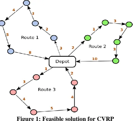
The capacitated vehicle routing problem (CVRP) is one of the most important combinatorial optimization problems which recently has been receiving much attention by researchers and scientists. CVRP deals with servicing a set of delivery customers or a set of pickup customers by a set of vehicles stationed at a central depot. Each vehicle, visits a set of customers such that every customer is visited exactly once and by exactly one vehicle. Furthermore, the capacity of each vehicle must not be violated. The objective of CVRP is to plan a set of routes to service all customers while minimizing the total travel distance. An example of a single solution consisting of a set of routes constructed for a CVRP is presented in Figure 1, where m=3 (number of vehicles) and n=14 (number of customers). To make CVRP models more realistic and applicable, there are many varieties of CVRP obtained by adding constraints to the basic model.
* Corresponding Author.
1 Department of Mathematics, Parand Branch, Islamic Azad University, Parand, Iran.
2 Department of Mathematics, Shahid Chamran University of Ahvaz, Iran.
Examples of such extensions are Asymmetric CVRP (ACVRP) if the cost matrix is not symmetric (Laporte et al., 1986), VRP with pickup and delivery if the vehicles need to pick up loads (Tang and Galvao, 2006), open VRP if the vehicles have not return to the depot (Li et al., 2007b), multi-depot VRP if the problem has multiple depots (Kuo and Wang, 2012), heterogeneous fleet VRP if capacity of vehicles are different (Subramanian et al., 2012), VRP with time windows if the services have time constraint (Hong, 2012), VRP with backhauls if the customers with delivery demand should be visited before the customers with pickup demand (Toth and Vigo, 1997), VRP with Mixed Pickup and Delivery (VRPMPD) if the delivery or pickup demand of some customers are set to zero (Nagy, and Salhi, 2005) and others.
The vehicle routing problem with pickup and delivery (VRPPD) is a variant of CVRP where customers require pick-up and delivery service from a single depotin which the vehicles are not only required to deliver goods to customers but also to pick some goods up at customer locations. The major difference between this problem and CVRP is that customers may receive or send goods, while in CVRP all customers just receive goods from a depot. In the context of these problems, customers who only receive goods are called delivery, while those only sending goods are called pickup, in many applications however customers will both send and receive goods. The core constraint of the VRPPD is that the capacity of the vehicle cannot be exceeded. Furthermore, other constraints such as maximum distance or time windows may exist may be considered in this problem. If customer distances and demands (these include both pickup and delivery demands) are given, the objective is to find a set of routes to minimize the total travelling cost while meeting customer demands.
Figure 1: Feasible solution for CVRP
Solving the Vehicle Routing Problem with Simultaneous Pickup and Delivery …
variant of the VRPPD, customers require simultaneous pick-up and delivery service from a single depotin which the vehicles are not only required to deliver goods to customers but also to pick some goods up at customer locations. Deliveries are supplied at the start of the vehicle’s service, while pick-up loads are taken to the same depot at the end of the service. One important characteristic of this problem is that a vehicle’s load in any given route is a mix of pick-up and delivery loads.
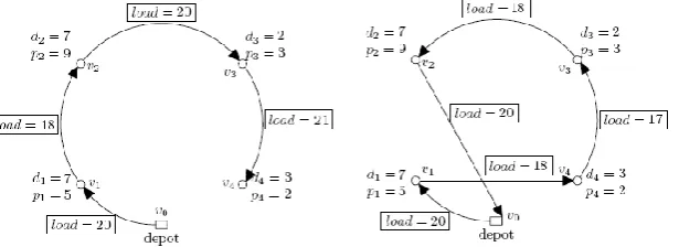
It should be noted that VRPSPD can be seen as a pickup and delivery problem (PDP) in the recent classification on static PDP by Berbeglia et al. (2007). VRPSPD is also called the multi-vehicle Hamiltonian one-to-many-to-one PDP with combined demands. By this definition, the deliveries are from the depot and the pickups will be returned to depot; the customer demand is combined which means that there is at least one customer with non-zero pickup and delivery demand. One obvious difference among CVRP, VRPB and VRPSDP is the variation of the vehicle load during the whole route. In CVRP, the load decreases (increases) monotonously while in the VRPB, it firstly decreases to zero and then starts to increase. Neither of the two cases is true in the VRPSDP. In this problem, the load of vehicles varies rulelessly and the maximum may appear in the middle of the route. Furthermore, if the total demand of all the customers assigned to the same vehicle does not exceed the capacity limit in CVRP, then the feasibility of the route would always behold, no matter what the visiting sequence is. Case in the VRPB is similar. However, it is quite different in the VRPSDP as we show in Figure 2. In this example, the vehicle capacity is 20 and the customers’ demands are defined. In this figure, the left side route is infeasible because the load of the vehicle exceeds its capacity after visiting customer v3, while the right side route is feasible where customer v3 is visited after v4. So the feasibility in the VRPSDP is not only related to the sum of the demands, but also strongly depends on the visiting order.
Figure 2: Feasible and infeasible examples for the VRPSDP
EACO overcome premature local optima encountered, several local search algorithms are employed. In this way, the proposed algorithm evolves towards diverse trajectories of the solution space, and a more extensive search is accomplished. The proposed framework was applied to 68 VRPSPD benchmark instances derived from the literature and involving from 50 to 200 customers. The results show the proposed algorithm not only obtained several of the best known solutions, but also presented very satisfying solutions for other instances.
The rest of this paper is organized as follows. In section 2, a mixed integer linear programming of VRPSPD is presented and the literature review is reported in section 3. In section 4, ACO and the EACO are explained and performance of the proposed algorithm will be described. The results of EACO will be compared with some of the other algorithms on standard problems in section 5. Finally, the conclusions are presented in section 6.
2. Problem formulation
From a graph theoretical point of view, we can define VRPSPD as follows. Let G = (V, E) be an undirected connected graph with V
0,1,..., n
as the set of vertexes and the set ofarcsE
(i, j):0i, jn
(if the graph is not complete, we can instead lack of each arc with thearc that has infinite size). Node 0 is the depot and the customer set C consists of n customers, i.e.,
C 1, 2,..., n . A nonnegative cost c (ij cii 0, 0 i n ) associated with each arc (i, j)E. 0
represents the depot and each customer has a demand di for delivery and pi for pickup. Let
C={1,2,…,m} be the set of homogeneous vehicles with capacity Q.
VRPSPD deals with finding the minimum total transportation cost for a set up to m routes so that the following constraints are taken into account:
The vehicles start to move simultaneously from the depot and return to the depot after visiting customers.
All the pickup and delivery demands are accomplished.
The vehicle’s capacity is not exceeded
Each customer is visited by only a single vehicle
The number of vehicles used cannot exceed m.
We present following mathematical formulation for HFFVRP using variablesx , P and ij ij
ij D where,
Error! Bookmark not defined. take the value 1 if denotele travels directly from customer i to customer j, and 0 otherwise; denotes the route. The flow non-negative variables Pij and Dijspecify the quantity of pickup and delivery goods that a vehicle is carrying when leaves customer i to service customer j.
0 0 min
ij
n n ij i j
c x (1)
01 1,...,
ij n
j
x i n (2)
01 j
n
j
x m (3)
0 0
0,...,
n n
ij ji
j j
x x i n (4)
0 0
1,...,
n n
ij ji i
j j
Solving the Vehicle Routing Problem with Simultaneous Pickup and Delivery …
0 0
1,...,
n n
ij ji i
j j
D D d i n (6)
1,..., , 1,...,
ij ij ij
P D Qx i n j n (7)
, 0 1,..., , 1,...,
ij ij
P D i n j n (8)
{0,1} 0,..., , 0,...,
ij
x i n j n (9)
The objective function (1) gives the sum of the total cost of the vehicles. Constraints (2) mean that only one arc can be exited for each customer; however, the maximum number of vehicles is guaranteed by constraints (3). Constraints (4) show that number of exited and entered arcs for each customer are same. Equality equations (5) and (6) insure that the quantity of pickup and delivery goods of each customer is fully satisfied in one visit. Constraints (7) state that the vehicle capacity is never exceeded. Restrictions (8) force the flow to remain non-negative and finally, constraints (9) describe that each arc in the network has the value 1 if it is used and 0 otherwise.
3.
Literature Review
VRPSPD was first proposed almost two decades ago by (Min, 1989). Min first inspired VRPSPD from a distribution problem of a public library, with one depot, two vehicles and 22 customers and presented a heuristic to solve for this real-life problem. His algorithm used to solve this problem involved the following stages:
(i) Customers are first clustered in such a way that the vehicle capacity is not exceeded in each group.
(ii) One vehicle is assigned to every cluster as Traveling Salesman Problem. (iii)The TSP is solved for each group of customers.
In during the algorithm, the infeasible arcs were penalized and the problems are resolved. Dell'Amico et al. (2006) firstly proposed an exact method based on column generation, dynamic programming, and branch and price method for this problem. However, the computational complexity of VRPSPD is evident from the computational result, in which an hour of computational time sometimes is not enough for solving a small size problem consist of 40 customers. Angelelli and Mansini (2002) also developed a branch-and-price algorithm for VRPSPD with time-windows constraints.
If Pj = 0 (j ∈ J), or even Pj ≤ Dj (j ∈ J) then the problem reduces to the VRP which is known to be NP-hard (Garey and Johnson, 1979), thus indicating that the VRPSDP is NP-hard, too. This means that the VRPSDP solution time grows exponentially with the increase in distribution points. In other words, the computational time required to solve adequately large problem instances is still prohibitive and heuristic methods become trapped in local optima and cannot gain a good suboptimal solution. Therefore, the focus of most researchers, is given to the design of meta-heuristic approaches capable of producing high quality near optimum solutions with reasonable computational time. As a result, many recent studies have been published on using advanced meta-heuristic techniques to solve VRPSPD. Some of the well-known meta-heuristics which have more ability for finding optimal solution are as follows:
Emmanouil et al. proposed a hybrid solution approach for VRPSPD incorporating the rationale of tabu search and guided local search which has proven to be effective for routing problem variants (Emmanouil et al., 2009). The performance of their meta-heuristic algorithm was tested on benchmark instances involving from 50 to 400 customers. Moreover, an improved differential evolution algorithm for solving VRPSPD with time window was proposed in (Mingyong and Erbao, 2010). In this algorithm, the novel decimal coding to construct an initial population is firstly adopted, and then used some improved differential evolution operators unlike the existing algorithm. A Large Neighborhood Search (LNS) heuristic associated with a procedure similar to the VNS meta-heuristic is developed to solve several variants of the VRP including VRPSPD (Ropke and Pisinger, 2004). Vural proposed some evolutionary based meta-heuristics for the problem such as two Genetic Algorithms in 2003. The first one is inspired on the random key technique while the second one consists in an improvement heuristic that applies Or-opt movements.
A modified ant colony algorithm is offered in which a new saving based visibility function and pheromone updating procedure (Catay, 2010). Zhang et al (2011) developed a new scatter search approach for the one of the most important extensions of VRPSPD called stochastic travel time VRPSPD by incorporating a new chance constrained programming method. They also proposed a genetic algorithm approach to this problem. In this paper, the Dethloff data will be used to evaluate the performance characteristics of both approaches.
Cruz et al. considered VRPSPD and applied a heuristic algorithm called GENVNS-TS-CL-PR. The proposed algorithm combines several heuristic algorithms, including cheapest insertion, cheapest insertion with multiple routes, GENIUS, variable neighborhood search, variable neighborhood descent, tabu search and path relinking (Cruz et al., 2012). In GENVNS-TS-CL-PR algorithm, first three procedures are used to obtain a high quality initial solution, and the last two algorithms are applied as local search methods. In more details, tabu search and path relinking are called after some iterations without any improvement through of the variable neighborhood search and after each variable neighborhood search iteration respectively, and it connects a local optimum with an elite solution generated during the search. The results showed that not only the algorithm was competitive other famous algorithms, but also it was able to generate high quality solutions for some standard instances.
Goksal et al., presented a heuristic solution algorithm based on particle swarm optimization in which a local search is performed by a variable neighborhood descent algorithm (VND) (Goksal et al., 2013). Moreover, it implements an annealing-like strategy to preserve the swarm diversity. The effectiveness of the proposed algorithm is investigated by an experiment conducted on benchmark problems available in the literature. The computational results indicate that the proposed algorithm competes with the heuristic approaches in the literature and improves several best known solutions.
Solving the Vehicle Routing Problem with Simultaneous Pickup and Delivery …
formulation was also presented. In addition, it is also shown how this formulation can be adapted to cater for other problem versions of VRP. Finally, various solution algorithms, including meta-heuristics were discussed to solve the models and what more is needed VRP.A variant of the basic VRP, where the vehicles serve delivery as well as pick up operations of the clients under time limit restrictions, is VRPSPD with Time Limit (VRPSPDTL). VRPSPDTL determines a set of vehicle routes originating and terminating at a central depot such that the total travel distance is minimized. For this problem, Polat et al (2015) presents a mixed-integer mathematical optimization model and a perturbation based neighborhood search algorithm combined with the classic savings heuristic, variable neighborhood search and a perturbation mechanism. The numerical results show that the proposed method produces superior solutions for a number of famous benchmark problems compared to those reported in the literature and reasonably good solutions for the remaining test problems.
The Vehicle Routing Problem with Mixed Pickup and Delivery (VRPMPD) differs from VRPSPD in that the customers may have either pickup or delivery demand. However, the solution approaches proposed for VRPSPD can be directly applied to the VRPMPD. In this paper, an adaptive local search solution approach is developed for both VRPSPD and the VRPMPD, which hybridizes a Simulated Annealing inspired algorithm with Variable Neighborhood Descent (Avci et al., 2015). The algorithm uses an adaptive threshold function that makes the algorithm self-tuning. The proposed approach is tested on well-known VRPSPD and VRPMPD benchmark instances derived from the literature.
Finally, Avci and Topaloglu considered an applied version of VRP called heterogeneous VRPSPD (Avci and Topaloglu, 2016). In this problem, the original version of VRPSPD is extended by assuming the fleet of vehicles to be heterogeneous. This problem, which can arise in many transportation systems involving both distribution and collection operations, is considered to be an NP-hard problem because it generalizes the classical VRP. So, a hybrid local search algorithm in which a non-monotone threshold adjusting strategy is integrated with tabu search was proposed for this new problem. In order to test the efficiency of the proposed algorithm, a set of randomly generated problem instances was considered and the results indicate that the developed algorithm obtains efficient and effective solutions.
4. Our algorithm
In this section, first, the ACO is presented and then the EACO will be analyzed in great detail.
4.1. Ant colony optimization
0
k i
ij ij k
i
k ij ij
ij
j N
k i
if j N P
if j N
(10)
Where
:
ij Amount of the pheromone of edge (i,j).
:
ij The inverse distance of edge (i,j).
Moreover, ants release “pheromone information”( ij) on the respective path while moving from node i to node j (formula (11)).
( ) ( )
ij t ij t ij (11)
The algorithm like its natural version makes use of pheromone evaporation in order to prevent the rapid convergence of ants to a sub-optimal path (formula (12)). Pheromone density is reduced in each iteration by 0 1 which is set by the user. In this formula, is the matrix for the existing pheromone on the edges of the respective graph.
(1 ) [0,1] (12)
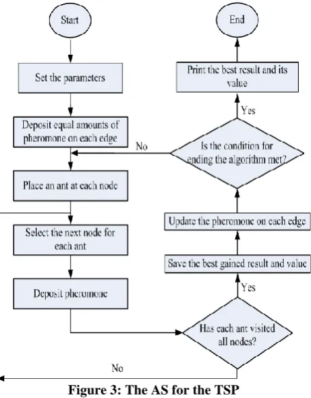
AS is the first version of ACO was applied in traveling salesman problem (TSP) because it was well adapted to this problem and a lot of algorithms have been implemented in TSP (Figure 3). Since AS could not produce acceptable results compared with meta-heuristic algorithms of the time such as Genetic Algorithm GA) and Simulated Algorithm (SA), several variants of ACO such as elite ant system (EAS), ACS, rank based ant system (RAS) and max-min ant system (MMAS) have been derived from the basic AS. These algorithms were able to produce better results for many combinatorial optimization problems, such as the scheduling problems (Merkle and Middendorf, 2003), assignment problems (Maniezzo and Carbonaro, 2000), and Vehicle Routing Problems (VRPs) (Gambardella et al., 1999).
4.2. Proposed Algorithm
Solving the Vehicle Routing Problem with Simultaneous Pickup and Delivery …
Figure 3: The AS for the TSP
(1) A new transition rule is introduced that favors exploration. From node i, the next node j in the route is selected by ant k, among the unvisited nodes k
i
N , according to the following transition
rule which shows the probability of each city being visited:
0
k i
ij ij ij k
i
k ij ij ij
ij
j N
k i
if j N P
if j N
(13)
Where
A control parameter set by the user 1
1
k k k
j j ij
ij k k
ij ij
p q
max{ . },
k k k k
ij pj qj s t j Ni
min{ . },
k k k k
ij pj qj s t j Ni
k j
p Pickup demand of customer j which is not visited by ant k.
k j
q Delivery demand of customer j which is not visited by ant k.
It is noted thatijkalways is between 0 and 1. Besides, if each unvisited customer j by ant k has a more value of pkj qkj, value of the ijkis increased. Here ijis defined inverse distance from the edge (I, j).
pheromone information by dynamically changing the desirability of paths. Using this rule, ants will search in a wide neighborhood of the best previous schedule. As the ant moves between nodes i and j, it updates the amount of pheromone on the traversed edge using the following formula:
0
( 1) (1 ). ( ) { ( , ) }
ij t ij t if edge i j Tk
(14) In this formula, the parameter0 1represents pheromone evaporation and deposited pheromone is discounted by a factor . It results in the new pheromone trail being a weighted average between the old pheromone value and the amount of pheromone deposited. Furthermore,
0
is the initial pheromone level assumed to be a small positive constant distributed equally on all the paths of the network since the start of the survey. The effect of local updating is that when an ant traverses an edge (i,j), its pheromone trail ij is reduced, so that the edges become less desirable for the ants in future iterations. This encourages an increase in the exploration of edges that have not been visited yet. Local updating helps avoid poor stagnation situations.
When all n groups of ants have completed their schedule and after using local search algorithms, the pheromone level is updated by applying the global updating rule only on the paths that belong to the best found solutions since the beginning. This proposed algorithm ranks the solutions constructed by ants. What distinguishes this algorithm from the other algorithms is the fact that in EACO the amount of releasing pheromone is based on the rank of the groups of ants in finding solutions. The formula is (15) instead of formula (12) in AS:
1
( 1) (1 ) ( ) ( )
ij t ij t ij t
(15)
Where:
( 1). ( , )
( ) ( )
0 ( , )
ij
Q
i j S L t
t
i j S
(16)
Q: A constant coefficient determined by the user.
: The number of groups of ants, which have been ranked and the pheromone has been deposited on their edges.
: The variable indicating ranking index from 1 to .S: The edges traversed by an ant group which has gained the
th rank in finding the best solution.In our EACO, best groups of ants of the algorithm have been allowed to lay pheromone on the arcs they traversed. The idea of the elitist strategy in the context of the proposed algorithm is to give extra emphasis to the best paths found so far in every iteration. This modification leads to balance between exploitation (through emphasizing global best ant) as well as exploration (through the emphasis to iteration best ant).
Solving the Vehicle Routing Problem with Simultaneous Pickup and Delivery …
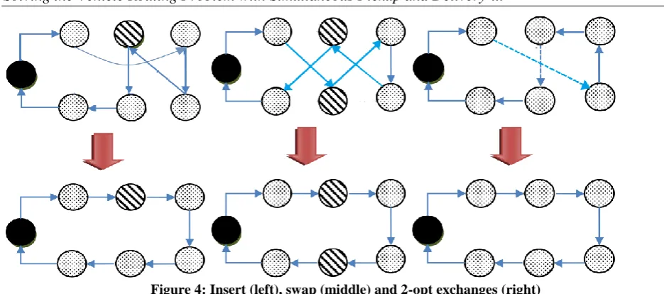
Figure 4: Insert (left), swap (middle) and 2-opt exchanges (right)
In insert algorithm, a customer is moved to another route (in Figure 4 (left).). However, in swap algorithm a customer in a certain route is swapped with another customer from a different route (in Figure 4 (middle)). One of the most commonly encountered moves is the 2-Opt. In multiple routes, two edges belong to a same route or different routes which form a criss-cross are selected and two new edges are replaced. This move is demonstrated in Figure 4 (right). It also should be noted that the new solution will be only accepted in state that first, VRPSPD constraints are not violated specially about each vehicle’s capacity and second, novel tour will gain better value for problem than previous solutions.
After each iteration, the stop condition is checked. If this condition is met, the algorithm ends. Otherwise, if stop conditions do not satisfy, the algorithm is iterated by returning to transition rule. To end the loop, the algorithm is iterated until the best solution is not changed 5 times. If the condition is met, the algorithm ends and the obtained results and values up to now are considered as the best values and results of the algorithm. The pseudo code of EACO for solving VRPSPD is presented in Figure 5.
Figure 5: The EACO for VRPSPD 1) Set the parameters.
2) For n groups, place m ants at n vertices randomly.
3) Select a nest node for each ant based on a new proposed formula and candidate list.
4) Deposit local pheromone.
5) If there is a node that has not been visited, go to step 3.
6) Save the best solution and its value obtained in current iteration. 7) Apply local search to the best solution in each iteration.
8) Update the best solution and its value obtained until now.
5. Numerical Analysis
At the first stage in this section, sensitivity analyses of parameters in the EACO are performed and at the second and third stages, the proposed algorithm, which is discussed in the previous section, is analyzed by using two sets of benchmark problems available in the literature for VRPSPD. The EACO is coded in Matlab 11 programming language and executed on a PC equipped with an Intel Pentium IV processor running at 3500 MHz; Core i3 and 8 GB of RAM running Microsoft Windows 7 Ultimate. Because the EACO is a meta-heuristic algorithm, the results are reported for ten independent runs and the best solution found in each instance is reported.
5.1. Sensitivity analyses of parameters
There are many parameters in the EACO affected by the final solution's quality. Consequently, a parameter setting procedure is necessary to reach the best balance between the qualities of the solutions. Because there is no way of defining the most effective values of the parameters, selections of some of the best parameters are considered and the best one is finally selected. We know that the most influential parameters in the proposed algorithm, which directly affect the quality of the final solution are , , , and
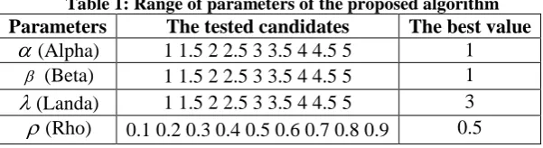
, so in this section, the parameters in our algorithm are tuned. The ranges of four parameters of the proposed algorithm are considered in Table 1 and the instance SCA8-6 was determined as the test problem. It is noted that the algorithm with each parameter is tested 10 times and the best solution is reported in Figure 6. In this figure, the horizontal axis shows the range of parameters and the vertical axis indicates the Gap of these algorithms. The Gap is computed by using formula (8) where c s( **) is the bestsolution found by each algorithm for a given instance, and c s( )* is the overall BKS for the same instance on the Web. A zero gap indicates that the best known solution of instance is found by the algorithm.
( **) * ( )* 100 ( )
c s c s Gap
c s
(17)
Based on the gained results shown in Figure 6 and column 3 in Table 1, the algorithm with the smaller weight parameter alpha of pheromone trails possesses higher performance. This may be attributed to that in the proposed algorithm the initial pheromone trails are large values. By using the large control factor of pheromone trail, the effect of visibility value is weakened and results in a premature convergence. In addition, the qualities of the solutions of the algorithms with Beta=1 and landa=3 are better than other parameters. Furthermore, from the test results, it can be found that by setting the evaporation factor to 0.5, the proposed algorithm can yield better solutions. This can be attributed to that if pheromone evaporation is too rapid or slow, it is more easily that result in the search to be trapped in local minimum. In other words, the suitable evaporation factor can ensure the sufficient diversity of search space and guide following ants to explore better solutions. As a result, the pack of optimal parameters obtained through several tests is shown in Table 1.
Table 1: Range of parameters of the proposed algorithm
Parameters The tested candidates The best value (Alpha) 1 1.5 2 2.5 3 3.5 4 4.5 5 1
(Beta) 1 1.5 2 2.5 3 3.5 4 4.5 5 1
(Landa) 1 1.5 2 2.5 3 3.5 4 4.5 5 3
Solving the Vehicle Routing Problem with Simultaneous Pickup and Delivery …
Figure 6: Parameters tuning of the proposed algorithm
5.2. The first data set of Benchmark instances
In this sub-section, the computational experiment is conducted on the benchmark data set of Dethloff (Dethloff, 2001). Instances are classified into four sets, namely SCA3, SCA8, CON3 and CON8. Each data set consists of 10 instances of a 50-customer problem. SCA data sets are generated with customers scattered uniformly in the service region of 100 _ 100. CON data sets are generated with half of the customers located uniformly in the service region and the other half are concentrated in the interval [100/3,100/3]. The delivery demand of customer i (di) is
generated from a uniform distribution in the interval [0,100] and then pickup demand (pi) is
calculated from the equation of pi = (0.5 + ri) di, where ri is a random number between [0, 1].
The numbers 3 and 8 after SCA or CON indicate the parameter for determining vehicle capacity. There are 10 problems in each group of problems. As mentioned earlier, VRPSPD is formulated by Dethloff as the problem to minimize the total traveled distance subject to the maximum capacity constraint of the vehicle. Hence, the following problem parameters are set as follows:
f = 0 (fixed cost per vehicle)
g=1 (variable cost per distance unit) D=∞ (service duration limit)
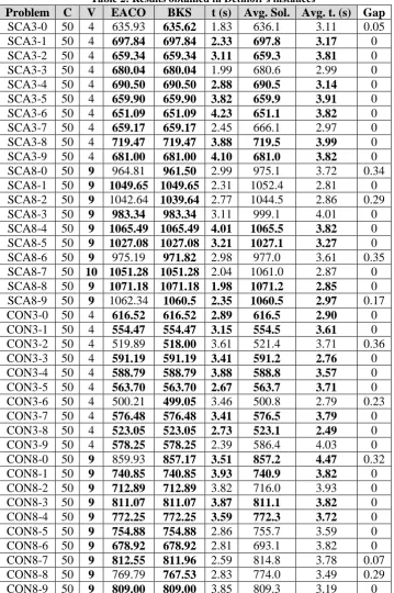
solutions was only 0.06% with the highest value in all the instances. It can be observed from Table 2 that among the 40 instances, the EACO has produced the high quality results of 10 instances and equaled another 30.
Table 2: Results obtained in Dethloff’s instances
Problem C V EACO BKS t (s) Avg. Sol. Avg. t. (s) Gap SCA3-0 50 4 635.93 635.62 1.83 636.1 3.11 0.05 SCA3-1 50 4 697.84 697.84 2.33 697.8 3.17 0 SCA3-2 50 4 659.34 659.34 3.11 659.3 3.81 0 SCA3-3 50 4 680.04 680.04 1.99 680.6 2.99 0 SCA3-4 50 4 690.50 690.50 2.88 690.5 3.14 0 SCA3-5 50 4 659.90 659.90 3.82 659.9 3.91 0 SCA3-6 50 4 651.09 651.09 4.23 651.1 3.82 0 SCA3-7 50 4 659.17 659.17 2.45 666.1 2.97 0 SCA3-8 50 4 719.47 719.47 3.88 719.5 3.99 0 SCA3-9 50 4 681.00 681.00 4.10 681.0 3.82 0 SCA8-0 50 9 964.81 961.50 2.99 975.1 3.72 0.34 SCA8-1 50 9 1049.65 1049.65 2.31 1052.4 2.81 0 SCA8-2 50 9 1042.64 1039.64 2.77 1044.5 2.86 0.29 SCA8-3 50 9 983.34 983.34 3.11 999.1 4.01 0 SCA8-4 50 9 1065.49 1065.49 4.01 1065.5 3.82 0 SCA8-5 50 9 1027.08 1027.08 3.21 1027.1 3.27 0 SCA8-6 50 9 975.19 971.82 2.98 977.0 3.61 0.35 SCA8-7 50 10 1051.28 1051.28 2.04 1061.0 2.87 0 SCA8-8 50 9 1071.18 1071.18 1.98 1071.2 2.85 0 SCA8-9 50 9 1062.34 1060.5 2.35 1060.5 2.97 0.17 CON3-0 50 4 616.52 616.52 2.89 616.5 2.90 0 CON3-1 50 4 554.47 554.47 3.15 554.5 3.61 0 CON3-2 50 4 519.89 518.00 3.61 521.4 3.71 0.36 CON3-3 50 4 591.19 591.19 3.41 591.2 2.76 0 CON3-4 50 4 588.79 588.79 3.88 588.8 3.57 0 CON3-5 50 4 563.70 563.70 2.67 563.7 3.71 0 CON3-6 50 4 500.21 499.05 3.46 500.8 2.79 0.23 CON3-7 50 4 576.48 576.48 3.41 576.5 3.79 0 CON3-8 50 4 523.05 523.05 2.73 523.1 2.49 0 CON3-9 50 4 578.25 578.25 2.39 586.4 4.03 0 CON8-0 50 9 859.93 857.17 3.51 857.2 4.47 0.32 CON8-1 50 9 740.85 740.85 3.93 740.9 3.82 0 CON8-2 50 9 712.89 712.89 3.82 716.0 3.93 0 CON8-3 50 9 811.07 811.07 3.87 811.1 3.82 0 CON8-4 50 9 772.25 772.25 3.59 772.3 3.72 0 CON8-5 50 9 754.88 754.88 2.86 755.7 3.59 0 CON8-6 50 9 678.92 678.92 2.81 693.1 3.82 0 CON8-7 50 9 812.55 811.96 2.59 814.8 3.78 0.07 CON8-8 50 9 769.79 767.53 2.83 774.0 3.49 0.29 CON8-9 50 9 809.00 809.00 3.85 809.3 3.19 0
Solving the Vehicle Routing Problem with Simultaneous Pickup and Delivery …
TS Tabu Search proposed by Tang and Galvao in 2006.
LNS Large Neighborhood Search proposed by Ropke and Pisinger in 2006.
PSO Particle Swarm Optimization proposed by Ai and Kachitvichyanukul in 2009. GA Genetic Algorithm proposed by Zhao et al. in 2009.
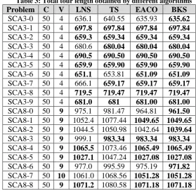
In this table, the first column includes the instance name, the second column (C) shows the number of customers, and the third column (V) presents the number of used vehicles, which for all of these instances is fixed at the minimum possible. It should be noted that these instances do not have the maximum route length restriction. The fourth and fifth columns of Table 3 are LNS and TS. The results of the EACO are in the seventh column and the last column includes the optimal values of these instances obtained in the literature (BKS). It should be noted that reported results for each instance is the best one over multiple runs. While LNS, TS and the proposed algorithm run 10 times for each instance.
The reason considering GA and PSO in the comparison to EACO is to draw a conclusion about performances of population-based heuristics in VRPSPD. It is also important to test the performance of the proposed algorithm against the TS and LNS since these meta-heuristic algorithms are the most effective algorithms recently proposed in the literature.
As can be seen from this table, the EACO finds the optimal solution for 30 out of 40 problems. The results also indicate that the proposed algorithm is a competitive approach compared to the LNS and TS. On the other hand, it is seen that LNS and TS fail to reach the best results for 18 and 23 out of 40 instances, respectively.
In 17 instances, both the EACO and TS are same. However, in other instances the proposed algorithm finds a better solution than TS. From this comparison we also conclude that the proposed method has better solution than the LNS for sixteen instances and equal solution for twenty two instances. As a result, the best algorithm is EACO which has found the best known solutions in 78%. The algorithms in terms of their performance from the worst to the best are: LNS, TS and EACO.
Table 3: Total tour length obtained by different algorithms
Problem C V LNS TS EACO BKS
Problem C V LNS TS EACO BKS SCA8-9 50 9 1060.5 1084.8 1062.34 1060.5 CON3-0 50 4 616.5 631.39 616.52 616.52 CON3-1 50 4 554.5 554.47 554.47 554.47 CON3-2 50 4 521.4 522.86 519.89 518.00 CON3-3 50 4 591.2 591.19 591.19 591.19 CON3-4 50 4 588.8 591.12 588.79 588.79 CON3-5 50 4 563.7 563.70 563.70 563.70 CON3-6 50 4 500.8 506.19 500.21 499.05 CON3-7 50 4 576.5 577.68 576.48 576.48 CON3-8 50 4 523.1 523.05 523.05 523.05 CON3-9 50 4 586.4 580.05 578.25 578.25 CON8-0 50 9 857.2 860.48 859.93 857.17 CON8-1 50 9 740.9 740.85 740.85 740.85 CON8-2 50 9 716.0 723.32 712.89 712.89 CON8-3 50 9 811.1 811.23 811.07 811.07 CON8-4 50 9 772.3 772.25 772.25 772.25 CON8-5 50 9 755.7 756.91 754.88 754.88 CON8-6 50 9 693.1 678.92 678.92 678.92 CON8-7 50 9 814.8 814.5 812.55 811.96 CON8-8 50 9 774.0 775.59 769.79 767.53 CON8-9 50 9 809.3 809 809.00 809.00
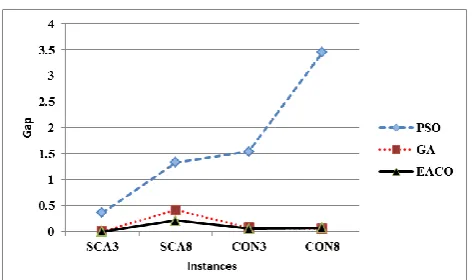
Because average result over the 10 instances for each data set was reported in (Ai and Kachitvichyanukul, 2009; Zhao et al., 2009), our results in the same way is presented to make a fair comparison of the heuristic approaches in Figure 7. Consequently, the relation average of percentage deviation (Gap) of PSO, GA and EACO from the BKS on specific benchmark instances is shown in the Figure 7. In this figure, the horizontal axis shows the name of four groups of instances and the vertical axis indicates the Gap of these algorithms. Generally, the results show that the PSO and GA have had a weak performance, but the results of the GA are much better than PSO. As a result, the EACO is the best algorithm and the performances from the worst to the best belong to PSO, GA and EACO. As it is shown in (Tarantilis et al. 2008), direct comparisons of the required computational times cannot be conducted as they closely depend on various factors such as the processing power of the computers, the programming languages, the coding abilities of the programmers, the compilers and the running processes on the computers.
Solving the Vehicle Routing Problem with Simultaneous Pickup and Delivery …
Figure 7: Comparison between PSO, GA and EACO for 4 groups of instances
Figure 8: Comparison of mean gap for PSO, GA and EACO
In order to further analyze the results of six mentioned algorithms, including PSO, GA and the proposed algorithm, one way analysis of variance (ANOVA) was conducted in order to determine if there are significant differences in the mean obtained solutions of the algorithms. This ANOVA analysis is conducted using the Minitab software in which the null hypothesis is that all means solutions of the three algorithms are equal, the alternative hypothesis is that at least one mean is different and the significance level is α = 0.05. In more details, equal variances were assumed for the analysis and rejecting the null hypothesis would mean that there is a significant difference between at least two of the algorithms. The results in Table 4 show that the p-value is 0.992, which is bigger than 0.05. Hence, the null hypothesis is not rejected when the level of significance is set at α = 0.05. In other words, there is no significant difference for mean of the all algorithms. Furthermore, it can be observed from Figure 9 that the proposed Algorithm is a little better than two other algorithms including GA and PSO.
Table 4: ANOVA of mean results of the three algorithms Source DF Adj SS Adj MS F-Value P-Value
Factor 2 549 274.6 0.01 0.992 Error 117 3846543 32876.4
EACO TS
LNS 1100
1000
900
800
700
600
500
D
at
a
Boxplot of LNS, TS, ...
EACO TS
LNS 820
800
780
760
740
720
700
D
at
a
Interval Plot of LNS, TS, ... 95% CI for the Mean
The pooled standard deviation is used to calculate the intervals.
Figure 9: Comparing results of the three algorithms for test problems
5.3. The second data set of Benchmark instances
The second data set of problem instances is suggested by Salhi and Nagy (1999). This data set has been modified from seven problems originally proposed by Christofides, Mingozzi, and Toth (1979) for the VRP with capacitated VRP. It is noted that these instances consist of 50 to 199 customers and the cost matrix is found by calculating the Euclidean distances between vertices. Salhi and Nagy (1999) utilize following scheme to modify capacitated VRP instances for VRPSPD: xi and yi coordinates for customer i are considered as in the original problem and a
ratio ri is calculated as ri=min (xi/yi, yi/xi). Let dmi be the demand of customer i. To obtain the
first 7 VRPSPD instances, namely X-series, the delivery and pickup quantities for customer i are calculated as di=ri .dmi and pi=(1-ri).dmi, respectively. The other seven VRPSPD instances,
namely Y-series, are generated by swapping the di and pi values for every customer (Gajpal &
Abad, 2009).
Table 5 shows the results of the proposed algorithm for VRPSPD instances. In this table, Columns 2-6 show the problem size C, the number of vehicles V, the best value result of the EACO, the CPU time of the MTSEAS for the best value result over the ten runs for each problem and the best known solutions (BKS). The most right column indicates the percentage of EACO improvement compared to the BKS (Gap). This table shows that the proposed algorithm can be used to solve VRPSPD effectively. In details, among the 28 instances, the EACO has produced the high quality results of 18 instances. Furthermore, it can be seen that among these test problems, the maximum relative error is 2.32% and the average relative error is 0.47%.
Table 5: Results of the MTSEAS for 14 VRPSPD instances
Instance C V Best solution Average
Solutions Time(s)
Average
Solving the Vehicle Routing Problem with Simultaneous Pickup and Delivery …
Instance C V Best solution Average
Solutions Time(s)
Average
Time(s) BKS Gap CMT12X 100 5 651.76 687.24 16.31 15.23 644.70 1.09 CMT13X 120 11 1551.25 1591.62 16.92 15.11 1551.25 0 CMT14X 100 10 821.75 832.48 13.78 14.67 821.75 0 CMT1Y 50 3 466.77 467.83 4.53 5.92 466.77 0 CMT2Y 75 6 663.25 663.25 8.23 7.25 663.25 0 CMT3Y 100 5 721.27 731.72 15.93 18.25 721.27 0 CMT4Y 150 7 852.46 899.73 28.71 35.72 852.35 0.01 CMT5Y 199 10 1033.55 1167.72 46.14 54.87 1029.25 0.42 CMT6Y 50 6 556.68 556.68 3.82 3.67 556.68 0 CMT7Y 75 11 901.22 904.72 6.82 5.83 901.22 0 CMT8Y 100 9 875.72 903.38 14.02 13.92 865.68 1.16 CMT9Y 150 15 1197.82 1278.52 24.82 29.73 1171.95 2.21 CMT10Y 199 19 1449.73 1565.62 41.92 50.41 1419.79 2.11 CMT11Y 120 4 832.63 887.62 21.72 28.34 830.39 0.27 CMT12Y 100 5a 659.52 687.19 18.25 19.26 659.52 0 CMT13Y 120 11 1583.61 1675.83 17.72 17.45 1547.75 2.32 CMT14Y 100 10 822.35 876.59 14.98 18.02 822.35 0
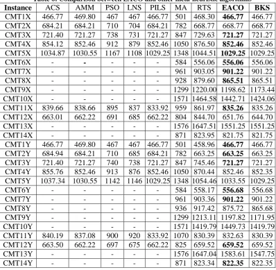
We utilize the best algorithms reported in the literature (as per our knowledge) to evaluate the performance of the proposed EACO for VRPSPD in Table 6:
RTS: Reactive tabu search (Wassan et al., 2008). ACS: Ant colony system (Gajpal & Abad, 2009).
AMM: Adaptive memory methodology (Zachariadis et al., 2010). PILS: Parallel iterative local search (Subramanian et al., 2010). PSO: Particle swarm optimization (Ai & Kachitvichyanukul, 2009a). LNS: Large neighborhood search (Ropke & Pisinger, 2006).
RTS: Reactive tabu search (Wassan et al., 2008).
MA: A mixed Insertion-based heuristics (Dethloff, 2001).
It is important to point out that Wassan et al. may have used another approach to generate the instance CMT1Y. The optimum solution of this instance (466.77) was found by means of the mathematical formulation presented in (Min, 1989). This value is greater than the one obtained by Wassan et al. (458.96). It should be noted that the optimum solution coincides with the solution found in (Subramanian et al., 2010), (Gajpal & Abad, 2009) and by the proposed algorithm. It can be observed from Table 4 that among the 14 instances, the proposed algorithm has obtained the best results of 10 instances from 14 instances.
Table 6: Comparison between EACO and other meta-heuristic algorithms
Instance ACS AMM PSO LNS PILS MA RTS EACO BKS
CMT1X 466.77 469.80 467 467 466.77 501 468.30 466.77 466.77 CMT2X 684.21 684.21 710 704 684.21 782 668.77 668.77 668.77 CMT3X 721.40 721.27 738 731 721.27 847 729.63 721.27 721.27 CMT4X 854.12 852.46 912 879 852.46 1050 876.50 852.46 852.46 CMT5X 1034.87 1030.55 1167 1108 1029.25 1348 1044.51 1029.25 1029.25
CMT6X - - - - - 584 556.06 556.06 556.06
CMT7X - - - 961 903.05 901.22 901.22
CMT8X - - - 928 879.60 865.51 865.51
CMT9X - - - 1299 1220.00 1198.62 1173.44 CMT10X - - - 1571 1464.58 1442.71 1424.06 CMT11X 839.66 838.66 895 837 833.92 959 861.97 835.26 835.26 CMT12X 663.01 662.22 691 685 662.22 804 844.70 651.76 644.70 CMT13X - - - 1576 1647.51 1551.25 1551.25 CMT14X - - - 871 823.95 821.75 821.75
CMT1Y 466.77 469.80 467 467 466.77 501 458.96 466.77 466.77 CMT2Y 684.94 684.21 710 685 684.21 782 663.25 663.25 663.25 CMT3Y 721.40 721.27 740 738 721.27 847 745.46 721.27 721.27 CMT4Y 855.76 852.46 913 876 852.46 1050 870.44 852.46 852.35 CMT5Y 1037.34 1030.55 1142 1146 1029.25 1348 1054.46 1033.55 1029.25
CMT6Y - - - 584 558.17 556.68 556.68
CMT7Y - - - 961 903.36 901.22 901.22
CMT8Y - - - 936 917.42 875.72 865.68
CMT9Y - - - 1299 1213.11 1197.82 1171.95 CMT10Y - - - 1571 1419.79 1449.73 1419.79 CMT11Y 840.19 837.08 900 920 833.92 1070 830.39 832.63 830.39 CMT12Y 663.50 662.22 697 675 662.22 825 659.52 659.52 659.52 CMT13Y - - - 1576 1647.04 1583.61 1547.75 CMT14Y - - - 871 823.34 822.35 822.35
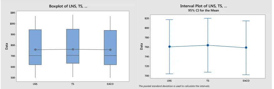
For better showing the quality of the proposed algorithm, the Gap of the obtained solutions are computed and compared to other solutions in Figure 10. From this Figure, we conclude that the EACO has the best deviation from the BKS in most of the instances. In more detail, the proposed HACO is the best algorithm which has found the best known solutions for all 15 out of 28
examples and is very competitive with other algorithms. However, in other instances, the
proposed algorithm finds nearly the BKS, i.e. the gap is about as high as 2.
Solving the Vehicle Routing Problem with Simultaneous Pickup and Delivery … -5 0 5 10 15 20 25 30 35 C M T 1X C M T 2X C M T 3X C M T 4X C M T 5X C M T 6X C M T 7X C M T 8X C M T 9X C M T 10 X C M T 11 X C M T 12 X C M T 13 X C M T 14 X C M T 1Y C M T 2Y C M T 3Y C M T 4Y C M T 5Y C M T 6Y C M T 7Y C M T 8Y C M T 9Y C M T 10 Y C M T 11 Y C M T 12 Y C M T 13 Y C M T 14 Y ACS AMM PSO LNS PILS MA RTS EACO
Figure 10: Comparison results of the algorithms
Figure 11: Comparison of mean gap for the algorithms
Table 7: ANOVA of mean common results of the eight algorithms Source DF Adj SS Adj MS F-Value P-Value Factor 7 285021 40717 1.09 0.373
Error 104 3874560 37255 Total 111 4159581
EACO RTS MA PILS LNS PSO AMM ACS 1400
1300
1200
1100
1000
900
800
700
600
500
D
at
a
Boxplot of ACS, AMM, ...
EACO RTS MA PILS LNS PSO AMM ACS 1000
900
800
700
600
D
at
a
Interval Plot of ACS, AMM, ... 95% CI for the Mean
The pooled standard deviation is used to calculate the intervals.
Figure 12: Comparing results of the eight algorithms for common test problems
6. Conclusion
In this research, we have proposed an effective ant colony optimization (EACO) that adopts a new state transition rule, a pheromone updating rule and three local search methods. A wide numerical experiment is performed on benchmark problem instances available in the literature. The proposed algorithm was tested in 68 benchmark problems with 50 to 199 customers and it was found capable of equaling with BKS for 48 instances. Computational results demonstrate that our algorithm has proven to be highly competitive in terms of quality of the solutions and CPU time for solving VRPSDP. Furthermore, this algorithm is effective compared to other meta-heuristics such as MA, LNS, PILS, PSO and ACS. It seems that combining the proposed algorithm with strong local algorithms like Lin-Kernigan algorithm can lead to better results for the proposed algorithm. Besides, some complex VRPSDP with more constraints such as time windows and multi-depots are a lot of research work in this field.
Acknowledgement
The authors would like to acknowledge the Parand Branch, Islamic Azad University for the financial support of this work.
References
Ai, T. J. and Kachitvichyanukul, V. 2009, “A particle swarm optimization for the vehicle routing problem with simultaneous pickup and delivery”, Computers & Operations Research, 36(5), 1693- 1702.
Angelelli, E. and Mansini R. 2002. “A branch-and-price algorithm for a simultaneous pick- up and delivery problem”, Quantitative approaches to distribution logistics and supply chain management. Berlin, Heidelberg: Springer, 249–267.
Avci, M. and Topaloglu, S. 2015, "An adaptive local search algorithm for vehicle routing problem with simultaneous and mixed pickups and deliveries", Computers & Industrial Engineering, 83, 15-29.
Solving the Vehicle Routing Problem with Simultaneous Pickup and Delivery …
Berbeglia, G., Cordeau, J. F., Gribkovskaia, I. and Laporte, G. 2007, “Static pickup and delivery problems: a classification scheme and survey”, TOP, 15(1), 1-31.
Bianchessi, N. and Righini. G. 2007, “Heuristic algorithms for the vehicle routing problem with simultaneous pickup and delivery”, Computers and Operations Research, 34(2), 578-594.
Brito, MP. and Dekker, R. 2004. @Reverse Logistics: a framework. In: Reverse logistics—quantitative models for closed-loop supply chains”, Berlin: Springer, 3–27.
Catay, B. 2010, “A new saving based ant algorithm for the vehicle routing problem with simultaneous pickup and delivery”, Expert Systems with Applications, 37, 6809–6817.
Christofides, N., Mingozzi, A. and Toth, P. 1979. The vehicle routing problem. In N. Christofides, A. Mingozzi, P. Toth, & L. Sandi (Eds.), Combinatorial optimization. Chichester, UK: Wiley.
Cruz, R.C., Silva, T.C.B.D., Souza, M.J., Coelho, V.N., Mine, M.T. and Martins, A.X., 2012. GENVNS-TS-CL-PR: A heuristic approach for solving the vehicle routing problem with simultaneous pickup and delivery. Electronic Notes in Discrete Mathematics, 39, 217-224.
Dell'Amico, M., Righini, G. and Salani, M. 2006, “A branch-and-price approach to the vehicle routing problem with simultaneous distribution and collection”, Transportation Science 40(2), 235-247.
Dethloff, J. 2001, “Vehicle routing and reverse logistics: the vehicle routing problem with simultaneous delivery and pick-up”, OR Spektrum, 23(1), 79-96.
Dorigo, M. 1992, “optimization, Learning and natural algorithms”, Ph.D Thesis, Dip.Electtronica e Informazion, Politecnico di Milano Italy.
Emmanouil, E. Z., Christos, D. T. and Chris. T. K. 2009, “A hybrid meta-heuristic algorithm for the vehicle routing problem with simultaneous delivery and pick-up service”, Expert Systems with Applications, 36(2), 1070-1081.
Gajpal, Y. and Abad, P. 2009, "An ant colony system (ACS) for vehicle routing problem with simultaneous delivery and pickup:, Computers and Operations Research, 36(12), 3215–3223.
Gambardella, M. Taillard, L. D. E. and Dorigo, M. 1999, “Ant colonies for the quadratic assignment problem”, Journal of the Operational Research Society, 50(2), 167–176.
Garey, M.R. and Johnson, D.S., 1979, “Computers and intractability: A guide to the theory of NP-completeness”, San Francisco: W.H. Freeman.
Goksal, F. P., Karaoglan, I. and Altiparmak, F. 2013, "A hybrid discrete particle swarm optimization for vehicle routing problem with simultaneous pickup and delivery", Computers & Industrial Engineering, 65(1), 39-53.
Hong, L. 2012, “An improved LNS algorithm for real-time vehicle routing problem with time windows”, Computers & Operations Research, 39(2), 151-163.
Kuo, Y. and Wang, C. C. 2012, “A variable neighborhood search for the multi-depot vehicle routing problem with loading cost”, Expert Systems with Applications, 39(8), 6949-6954.
Laporte, G., Mercure, H. and Nobert, Y. 1986, “An exact algorithm for the asymmetrical capacitated vehicle routing problem”, Networks, 16, 33–46
Li, F., Golden, B. and Wasil, E. 2007b, “The open vehicle routing problem: Algorithms, large-scale test problems, and computational results”, Computers and Operations Research, 34, 2918–2930.
Min, H. 1989, "The multiple vehicle routing problem with simultaneous delivery and pick-up points", Transportation Research A, 23(5), 377-386.
Maniezzo, V. and Carbonaro, A. 2000, “An ants heuristic for the frequency assignment problem”, Future Generation Computer Systems, 16(8), 927–935.
Merkle, D. and Middendorf, M. 2003, “Ant colony optimization with global pheromone evaluation for scheduling a single machine”, Applied Intelligence, 18(1), 105–111.
Min, H. 1989, “The multiple vehicle routing problem with simultaneous delivery and pick-up points”, Transportation Research A, 23(5), 377-386.
Nagy, G. and Salhi, S. 2005, “Heuristic algorithm for single and multiple depot vehicle routing problem with pickups and deliveries”, European Journal of Operational Research, 162, 126–141.
Polat, O., Kalayci, C. B. Kulak, O. and Günther, H. O. 2015, "A perturbation based variable neighborhood search heuristic for solving the Vehicle Routing Problem with Simultaneous Pickup and Delivery with Time Limit", European Journal of Operational Research, 242(2), 369-382
Repoussis, P. P., Tarantilis, C. D. and Ioannou, G. 2006, “The open vehicle routing problem with time windows”, Journal of the Operational Research Society, 58, 355-367.
Ropke, S. and Pisinger, D. 2004, “A unified heuristic for a large class of vehicle routing problems with backhauls”, Technical Report 2004/14, University of Copenhagen.
Salhi, S. and Nagy, G. 1999, “A cluster insertion heuristic for single and multiple depot vehicle routing problems with backhauling”, Journal of the Operational Research Society, 50(10), 1034-1042.
Subramanian, A., Drummonda, L. M. A., Bentes, C., Ochi, L. S. and Farias, R. 2010, "A parallel heuristic for the Vehicle Routing Problem with Simultaneous Pickup and Delivery", Computers & Operations Research, 37, 1899–1911.
Subramanian, A., Huachi, P., Penna, V., Uchoa, E. and Ochi, L. S. 2012, “A hybrid algorithm for the Heterogeneous Fleet Vehicle Routing Problem”, European Journal of Operational Research, 221(2), 285-295.
Tang, FA. and Galvao, RD. 2006, “A tabu search algorithm for the vehicle routing problem with simultaneous pick-up and delivery service”, Computers and Operations Research, 33(3), 595–619.
Tarantilis, C., Zachariadis, E. and Kiranoudis, C. 2008, “A guided Tabu search for the heterogeneous vehicle routing problem”, Journal of the Operational Research Society, 59, 1659-1673.
Toth, P. and Vigo, D. 1997, “An exact algorithm for the vehicle routing problem with backhauls”, Transportation Science, 31, 372–385.
Vural, AV. 2003). “A GA based meta-heuristic for capacitated vehicle routing problem with simultaneous pickup and deliveries”, Master’s thesis, Graduate School of Engineering and Natural Sciences, Sabanci University.
Wassan, N. A., Wassan, A. H., Nagy, G. 2008, "A reactive tabu search algorithm for the vehicle routing problem with simultaneous pickups and deliveries", Journal of Combinatorial Optimization, 15(4), 368– 386.
Wassan, N.A. and Nagy, G. 2014. “Vehicle routing problem with deliveries and pickups: Modelling issues and meta-heuristics solution approaches”, International Journal of Transportation, 2(1), 95-110. Zachariadis, E. E., Tarantilis, C. D., Kiranoudis, C. T. 2009, "A hybrid meta-heuristic algorithm for the vehicle routing problem with simultaneous delivery and pick-up service", Expert Systems with Applications, 36(2), 1070–1081.
Zhang, T., Chaovalitwongse, W. A. and Zhang, Y. 2011, “Scatter search for the stochastic travel time vehicle routing problem with simultaneous pickups and deliveries”, Computers & Operations Research, 39, 2277–2290.
Zhao, F., Mai, D., Dun J. and Liu, W. 2009, “A hybrid genetic algorithm for the vehicle routing problem with simultaneous pickup and delivery”, Chinese Control and Decision Conference, CCDC 2009, 3928-